An adaptive finite element PML method for the acoustic-elastic interaction in three dimensions

Abstract.

Consider the scattering of a time-harmonic acoustic incident wave by a bounded, penetrable, and isotropic elastic solid, which is immersed in a homogeneous compressible air or fluid. The paper concerns the numerical solution for such an acoustic-elastic interaction problem in three dimensions. An exact transparent boundary condition (TBC) is developed to reduce the problem equivalently into a boundary value problem in a bounded domain. The perfectly matched layer (PML) technique is adopted to truncate the unbounded physical domain into a bounded computational domain. The well-posedness and exponential convergence of the solution are established for the truncated PML problem by using a PML equivalent TBC. An a posteriori error estimate based adaptive finite element method is developed to solve the scattering problem. Numerical experiments are included to demonstrate the competitive behavior of the proposed method.

1. Introduction

Consider the incidence of a time-harmonic acoustic wave onto a bounded, penetrable, and isotropic elastic solid, which is immersed in a homogeneous and compressible air or fluid. Due to the interaction between the incident wave and the solid obstacle, an elastic wave is excited inside the solid region, while the acoustic incident wave is scattered in the air/fluid region. This scattering phenomenon leads to an air/fluid-solid interaction problem. The surface of the elastic solid divides the whole three-dimensional space into a bounded interior domain and an open exterior domain where the elastic wave and the acoustic wave occupies, respectively. The two waves are coupled together on the surface via the interface conditions: continuity of the normal component of velocity and the continuity of traction. The acoustic-elastic interaction problems have received ever-increasing attention due to their significant applications in geophysics and seismology [22, 23]. These problems have been examined mathematically by using either variational method [18, 19] or boundary integral equation method [28, 24]. Many computational approaches have also been developed to numerically solve these problems such as boundary element method [17, 31] and coupling of finite and boundary element methods [16].

Since the work by Bérenger [4], the perfectly matched layer (PML) technique has been extensively studied and widely used to simulate various wave propagation problems, which include acoustic waves [5, 12, 21, 27, 32], elastic waves [6, 11, 13, 20, 26], and electromagnetic waves [3, 15]. The PML is to surround the domain of interest by a layer of finite thickness fictitious material which absorbs all the waves coming from inside the computational domain. It has been proven to be an effective approach to truncated open domains in the wave computation. Combined with the PML technique, the adaptive finite element method (FEM) has recently been developed to solve the diffraction grating problems [2, 8, 25] and the obstacle scattering problems [7, 9, 10]. Despite the large number of work done so far, they were concerned with a single wave propagation problem, i.e., either an acoustic wave, or an elastic wave, or an electromagnetic wave. It is very rare to study rigorously the PML problem for the interaction of multiple waves.

This paper aims to investigate the adaptive finite element PML method for solving the acoustic-elastic interaction problem. An exact transparent boundary condition (TBC) is developed to reduce the problem equivalently into a boundary value problem in a bounded domain. The PML technique is adopted to truncated the unbounded physical domain into a bounded computational domain. The variational approach is taken to incorporate naturally the interface conditions which couple the two waves. The well-posedness and exponential convergence of the solution are established for the truncated PML problem by using a PML equivalent TBC. The proofs rely on the error estimate between the two transparent boundary operators. To effciently resolve the solution with possible singularities, the a posteriori error estimate based adaptive FEM is developed to solve the truncated PML problem. The error estimate consists of the PML error and the finite element discretization error, and provides a theoretical basis for the mesh refinement. Numerical experiments are reported to show the competitive behavior of the proposed method.

The paper is organized as follows. In section 2, we introduce the model equations for the acoustic-elastic interaction problem. In section 3, we present the PML formulation and prove the well-posedness and convergence of the solution for the truncated PML problem. In section 4, we discuss the numerical implementation and show some numerical experiments. The paper is concluded with some general remarks in section 5.

2. Problem formulation

In this section, we introduce the model equations for acoustic and elastic waves, and present an interface problem for the acoustic-elastic interaction. In addition, an exact transparent boundary condition is introduced to reformulate the scattering problem into an boundary value problem in an bounded domain.

2.1. Problem geometry

Consider an acoustic plane wave incident on a bounded elastic solid which is immersed in a homogeneous compressible air/fluid in three dimensions. The problem geometry is shown in Figure 1. Due to the wave interaction, an elastic wave is induced inside the solid region, while the scattered acoustic wave is generated in the open air/fluid region. The wave propagation described above leads to an air/fluid-solid interaction problem. The surface of the solid divides the whole three-dimensional space into the interior domain and the exterior domain, where the elastic wave and the acoustic wave occupies, respectively. Let the solid $\Omega_{s}\subset\mathbb{R}^{3}$ be a bounded domain with a Lipschitz boundary $\Gamma_{s}$. The exterior domain $\Omega_{e}=\mathbb{R}^{3}\setminus\bar{\Omega}_{s}$ is assumed to be connected and filled with a homogeneous, compressible, and inviscid air/fluid with a constant density $\rho_{a}>0$. Denote by $B=\{\boldsymbol{x}=(x_{1},x_{2},x_{3})^{\top}\in\mathbb{R}^{3}:|x_{j}|<L_{j},j=1,2,3\}$ the rectangular box with the boundary $\partial B$, where $L_{j}$ are sufficiently large such that $\bar{\Omega}_{s}\subset B$. Define $\Omega_{a}=B\setminus\bar{\Omega}_{s}$. Let $\boldsymbol{n}_{1}$ be the unit normal vector on $\Gamma_{s}$ directed from $\Omega_{s}$ into $\Omega_{e}$, and let $\boldsymbol{n}_{2}$ be the unit outward normal vector on $\partial B$.

Figure 1. A two-dimensional schematic of the problem geometry for the acoustic-elastic interaction.

2.2. Wave equations

Let the elastic solid be impinged by a time-harmonic sound wave $p^{\rm inc}$, which satisfies the three-dimensional Helmholtz equation:

$$\Delta p^{\rm inc}+\kappa^{2}p^{\rm inc}=0\quad\text{in}~{}\Omega_{e},$$

where $\kappa=\omega/c$ is the wavenumber, $\omega>0$ is the angular frequency, and $c$ is the speed of sound in the air/fluid. The total acoustic wave field $p$ also satisfies the Helmholtz equation:

$$\Delta p+\kappa^{2}p=0\quad\text{in}~{}\Omega_{e}.$$ (2.1)

The total field $p$ consists of the incident field $p^{\rm inc}$ and the scattered field $p^{\rm sc}$:

$$p=p^{\rm inc}+p^{\rm sc}\quad\text{in}~{}\Omega_{e},$$

where scattered field $p^{\rm sc}$ is required to satisfy the Sommerfeld radiation condition:

$$\lim_{r\to\infty}r(\partial_{r}p^{\rm sc}-{\rm i}\kappa p^{\rm sc})=0,\quad r=|\boldsymbol{x}|.$$

The time-harmonic elastic wave satisfies the three-dimensional Navier equation:

$$\nabla\cdot\boldsymbol{\sigma}(\boldsymbol{u})+\omega^{2}\boldsymbol{u}=0\quad\text{in}~{}\Omega_{s},$$ (2.2)

where $\boldsymbol{u}=(u_{1},u_{2},u_{3})^{\top}$ is the displacement of the elastic wave, and the stress tensor $\boldsymbol{\sigma}(\boldsymbol{u})$ is given by the generalized Hook law:

$$\boldsymbol{\sigma}(\boldsymbol{u})=2\mu\boldsymbol{\epsilon}(\boldsymbol{u})+\lambda{\rm tr}(\boldsymbol{\epsilon}(\boldsymbol{u}))I,\quad\boldsymbol{\epsilon}(\boldsymbol{u})=\frac{1}{2}(\nabla\boldsymbol{u}+\nabla\boldsymbol{u}^{\top}).$$ (2.3)

Here $\mu(\boldsymbol{x})\in L^{\infty}(\Omega_{s}),\lambda(\boldsymbol{x})\in L^{\infty}(\Omega_{s})$ are the Lamé parameters satisfying $\mu>0,\lambda>0$, and $\nabla\boldsymbol{u}$ is the displacement gradient tensor given by

$$\nabla\boldsymbol{u}=\begin{bmatrix}\partial_{x_{1}}u_{1}&\partial_{x_{2}}u_{1}&\partial_{x_{3}}u_{1}\\ \partial_{x_{1}}u_{2}&\partial_{x_{2}}u_{2}&\partial_{x_{3}}u_{2}\\ \partial_{x_{1}}u_{3}&\partial_{x_{2}}u_{3}&\partial_{x_{3}}u_{3}\end{bmatrix}.$$

Substituting (2.3) into (2.2) yields

$$\nabla\cdot(\mu(\nabla\boldsymbol{u}+\nabla\boldsymbol{u}^{\top}))+\nabla(\lambda\nabla\cdot\boldsymbol{u})+\omega^{2}\boldsymbol{u}=0\quad\text{in}~{}\Omega_{s}.$$ (2.4)

2.3. Interface conditions

To couple the acoustic wave equation and the elastic wave equation, the kinematic interface condition is imposed to ensure the continuity of the normal component of the velocity:

$$\partial_{\boldsymbol{n}_{1}}p=\rho_{a}\omega^{2}\boldsymbol{n}_{1}\cdot\boldsymbol{u}\quad\text{on}~{}\Gamma_{s},$$ (2.5)

In addition, the dynamic interface condition is required to ensure the continuity of traction:

$$-p\boldsymbol{n}_{1}=\boldsymbol{\sigma}(\boldsymbol{u})\cdot\boldsymbol{n}_{1}\quad\text{on}~{}\Gamma_{s},$$ (2.6)

where $\boldsymbol{\sigma}(\boldsymbol{u})\cdot\boldsymbol{n}_{1}$ denotes the matrix-vector multiplication.

2.4. Acoustic-elastic interaction problem

The acoustic-elastic interaction problem can be formulated into the following coupled boundary value problem: Given $p^{\rm inc}$, to find $(p,\boldsymbol{u})$ such that

$$\begin{cases}\Delta p+\kappa^{2}p=0,\quad p=p^{\rm inc}+p^{\rm sc}&\quad\text{in}~{}\Omega_{e},\\ \nabla\cdot\boldsymbol{\sigma}(\boldsymbol{u})+\omega^{2}\boldsymbol{u}=0&\quad\text{in}~{}\Omega_{s},\\ \partial_{\boldsymbol{n}_{1}}p=\rho_{a}\omega^{2}\boldsymbol{n}_{1}\cdot\boldsymbol{u},\quad-p\boldsymbol{n}_{1}=\boldsymbol{\sigma}(\boldsymbol{u})\cdot\boldsymbol{n}_{1}&\quad\text{on}~{}\Gamma_{s},\\ \partial_{r}p^{\rm sc}-{\rm i}\kappa p^{\rm sc}=o(r^{-1})&\quad\text{as}~{}r\to\infty.\end{cases}$$ (2.7)

We refer to [28] for the discussion on the well-posedness of the boundary value problem (2.7). From now on, we assume that the acoustic-elastic interaction problem has a unique solution.

2.5. Transparent boundary condition

Given $v\in H^{1/2}(\partial B)$, we define the Dirichlet-to-Neumann (DtN) operator $\mathscr{T}:H^{1/2}(\partial B)\to H^{-1/2}(\partial B)$ as follows:

$$\mathscr{T}v=\partial_{\boldsymbol{n}_{2}}u\quad\text{on}~{}\partial B,$$

where $u$ is the solution of the exterior Dirichlet problem of the Helmholtz equation:

$$\begin{cases}\Delta u+\kappa^{2}u=0&\quad\text{in}~{}\mathbb{R}^{3}\setminus\bar{B},\\ u=v&\quad\text{on}~{}\partial B,\\ \partial_{r}u-{\rm i}\kappa u=o(r^{-1})&\quad\text{as}~{}r\to\infty.\end{cases}$$ (2.8)

It is well-known that the exterior problem (2.8) has a unique solution $u\in H^{1}_{loc}(\mathbb{R}^{3}\setminus\bar{B})$ (cf., e.g., [14]). Thus the DtN operator $\mathscr{T}:H^{1/2}(\partial B)\to H^{-1/2}(\partial B)$ is well-defined and is a bounded linear operator.

Using the DtN operator $\mathscr{T}$, we reformulate the boundary value problem (2.7) from the open domain into the bounded domain: Given $p^{\rm inc}$, to find $(p,\boldsymbol{u})$ such that

$$\begin{cases}\Delta p+\kappa^{2}p=0&\quad\text{in}~{}\Omega_{a},\\ \nabla\cdot\boldsymbol{\sigma}(\boldsymbol{u})+\omega^{2}\boldsymbol{u}=0&\quad\text{in}~{}\Omega_{s},\\ \partial_{\boldsymbol{n}_{1}}p=\rho_{a}\omega^{2}\boldsymbol{n}_{1}\cdot\boldsymbol{u},\quad-p\boldsymbol{n}_{1}=\boldsymbol{\sigma}(\boldsymbol{u})\cdot\boldsymbol{n}_{1}&\quad\text{on}~{}\Gamma_{s},\\ \partial_{\boldsymbol{n}_{2}}p=\mathscr{T}p+f&\quad\text{on}~{}\partial B,\end{cases}$$ (2.9)

where $f=\partial_{\boldsymbol{n}_{2}}p^{\rm inc}-\mathscr{T}p^{\rm inc}$.

To study the well-posedness of (2.9), we define

$$\boldsymbol{X}:=H^{1}(\Omega_{a})\times H^{1}(\Omega_{s})^{3}=\{\boldsymbol{\Phi}=(p,\boldsymbol{u}):p\in H^{1}(\Omega_{a}),\boldsymbol{u}\in H^{1}(\Omega_{s})^{3}\},$$

which is endowed with the inner product:

$$(\boldsymbol{\Phi},\boldsymbol{\Psi})_{\boldsymbol{X}}:=\int_{\Omega_{a}}\left(\nabla p\cdot\nabla\bar{q}+p\bar{q}\right){\rm d}\boldsymbol{x}+\int_{\Omega_{s}}\left(\nabla\boldsymbol{u}:\nabla\bar{\boldsymbol{v}}+\boldsymbol{u}\cdot\bar{\boldsymbol{v}}\right){\rm d}\boldsymbol{x}$$

for any $\boldsymbol{\Phi}=(p,\boldsymbol{u})$ and $\boldsymbol{\Psi}=(q,\boldsymbol{v})$, where $A:B={\rm tr}(AB^{\top})$ is the Frobenius inner product of square matrices $A$ and $B$. Clearly, $\|\cdot\|_{\boldsymbol{X}}=\sqrt{(\cdot,\cdot)_{\boldsymbol{X}}}$ is a norm on $\boldsymbol{X}$.

Let $a:\boldsymbol{X}\times\boldsymbol{X}\to\mathbb{C}$ be the sesquilinear form:

$$a(p,\boldsymbol{u};q,\boldsymbol{v})= \int_{\Omega_{a}}\left(\nabla p\cdot\nabla\bar{q}-\kappa^{2}p\bar{q}\right){\rm d}\boldsymbol{x}+\int_{\Gamma_{s}}\rho_{a}\omega^{2}(\boldsymbol{n}_{1}\cdot\boldsymbol{u})\bar{q}{\rm d}s-\int_{\partial B}(\mathscr{T}p)\bar{q}{\rm d}s$$

$$+\int_{\Omega_{s}}\left(\boldsymbol{\sigma}(\boldsymbol{u}):\nabla\bar{\boldsymbol{v}}-\omega^{2}\boldsymbol{u}\cdot\bar{\boldsymbol{v}}\right){\rm d}\boldsymbol{x}+\int_{\Gamma_{s}}(p\boldsymbol{n}_{1})\cdot\bar{\boldsymbol{v}}{\rm d}s.$$ (2.10)

The acoustic-elastic interaction problem (2.9) is equivalent to the following weak formulation: Find $\boldsymbol{\Phi}=(p,\boldsymbol{u})\in\boldsymbol{X}$ such that

$$a(p,\boldsymbol{u};q,\boldsymbol{v})=\int_{\partial B}f\bar{q}{\rm d}s,\quad\forall\,\boldsymbol{\Psi}=(q,\boldsymbol{v})\in\boldsymbol{X}.$$ (2.11)

Since we assume that the variational problem (2.11) has a unique weak solution $(p,\boldsymbol{u})\in\boldsymbol{X}$, the general theory in Babuška and Aziz [1, Chap. 5] implies that there exists a constant $\gamma_{0}$ such that the following inf-sup condition is satisfied

$$\sup_{0\neq(q,\boldsymbol{v})\in\boldsymbol{X}}\frac{|a(p,\boldsymbol{u};q,\boldsymbol{v})|}{\|(q,\boldsymbol{v})\|_{\boldsymbol{X}}}\geq\gamma_{0}\|(p,\boldsymbol{u})\|_{\boldsymbol{X}},\quad\forall\,(p,\boldsymbol{u})\in\boldsymbol{X}.$$ (2.12)

3. The PML problem

In this section, we introduce the PML formulation for the acoustic-elastic interaction problem and establish its well-posedness. An error estimate will be shown for the solutions between the original scattering problem and the PML problem.

3.1. PML formulation

Now we turn to the introduction of an absorbing PML layer. As is shown in Figure 2, the domain $\Omega_{a}$ is surrounded by a PML layer of thickness $d_{j}$ which is denoted as $\Omega_{\rm PML}$. Define $\Omega:=\Omega_{a}\cup\partial B\cup\Omega_{\rm PML}$. Let $\alpha_{j}(t)=1+{\rm i}\sigma_{j}(t)$ be the PML function which is continuous and satisfies

$$\sigma_{j}(t)=0\quad\text{for}~{}|t|<L_{j}\quad\text{and}\quad\sigma_{j}(t)=\sigma_{0}\left(\frac{|t|-L_{j}}{d_{j}}\right)^{m}\quad\text{otherwise}.$$

Here $\sigma_{0}>0$ is a constant and $m$ is an integer. Following [15], we introduce the PML by the complex coordinate stretching:

$$\tilde{x}_{j}=\int_{0}^{x_{j}}\alpha_{j}(\tau){\rm d}\tau,\quad 1\leq j\leq 3.$$ (3.1)

Figure 2. A two-dimensional schematic of the geometry for the PML problem.

Let $\tilde{\boldsymbol{x}}=(\tilde{x}_{1},\tilde{x}_{2},\tilde{x}_{3})$. Introduce the new function:

$$\tilde{p}(\boldsymbol{x})=\begin{cases}p^{\rm inc}(\boldsymbol{x})+(p(\tilde{\boldsymbol{x}})-p^{\rm inc}(\tilde{\boldsymbol{x}})),\quad&\boldsymbol{x}\in\Omega_{\rm PML},\\ p(\tilde{\boldsymbol{x}}),\quad&\boldsymbol{x}\in\Omega_{a}.\end{cases}$$ (3.2)

It is clear to note that $\tilde{p}({\boldsymbol{x}})=p(\boldsymbol{x})$ in $\Omega_{a}$ since $\tilde{\boldsymbol{x}}=\boldsymbol{x}$ in $\Omega_{a}$. It can be verified from (2.1) and (3.1) that $\tilde{p}$ satisfies

$$\mathscr{L}(\tilde{p}-p^{\rm inc})=0\quad\text{in}~{}\Omega,$$

where the PML differential operator is defined by

$$\mathscr{L}p=\nabla\cdot(A\nabla p)+\kappa^{2}bp,$$

where

$$A={\rm diag}\left(\frac{\alpha_{2}\alpha_{3}}{\alpha_{1}},\frac{\alpha_{1}\alpha_{3}}{\alpha_{2}},\frac{\alpha_{1}\alpha_{2}}{\alpha_{3}}\right),\quad b=\alpha_{1}\alpha_{2}\alpha_{3}.$$

It can be verified from (2.1) and (3.2) that the outgoing wave $\tilde{p}(\boldsymbol{x})-p^{\rm inc}(\boldsymbol{x})$ in $\Omega_{\rm PML}$ decays exponentially. Therefore, the homogeneous Dirichlet boundary condition can be imposed on $\Gamma:=\partial\Omega_{\rm PML}\setminus\partial B$ to truncate the PML problem. We arrive at the following truncated PML problem: Find $(\hat{p},\hat{\boldsymbol{u}})$ such that

$$\begin{cases}\mathscr{L}\hat{p}=g&\quad\text{in}~{}\Omega,\\ \nabla\cdot\boldsymbol{\sigma}(\hat{\boldsymbol{u}})+\omega^{2}\hat{\boldsymbol{u}}=0&\quad\text{in}~{}\Omega_{s},\\ \partial_{\boldsymbol{n}_{1}}\hat{p}=\rho_{a}\omega^{2}\boldsymbol{n}_{1}\cdot\hat{\boldsymbol{u}},\quad-\hat{p}\boldsymbol{n}_{1}=\boldsymbol{\sigma}(\hat{\boldsymbol{u}})\cdot\boldsymbol{n}_{1}&\quad\text{on}~{}\Gamma_{s},\\ \hat{p}=p^{\rm inc}&\quad\text{on}~{}\Gamma,\end{cases}$$ (3.3)

where

$$g=\begin{cases}\mathscr{L}p^{\rm inc}&\quad\text{in}~{}\Omega_{\rm PML},\\ 0&\quad\text{in}~{}\Omega_{a}.\end{cases}$$

Define

$$\boldsymbol{Y}:=H^{1}(\Omega)\times H^{1}(\Omega_{s})^{3}=\{\boldsymbol{\Phi}=(p,\boldsymbol{u}):p\in H^{1}(\Omega),\boldsymbol{u}\in H^{1}(\Omega_{s})^{3}\},$$

which is endowed with the inner product

$$(\boldsymbol{\Phi},\boldsymbol{\Psi})_{\boldsymbol{Y}}:=\int_{\Omega}\left(\nabla p\cdot\nabla\bar{q}+p\bar{q}\right){\rm d}\boldsymbol{x}+\int_{\Omega_{s}}\left(\nabla\boldsymbol{u}:\nabla\bar{\boldsymbol{v}}+\boldsymbol{u}\cdot\bar{\boldsymbol{v}}\right){\rm d}\boldsymbol{x}$$

for any $\boldsymbol{\Phi}=(p,\boldsymbol{u})$ and $\boldsymbol{\Psi}=(q,\boldsymbol{v})$. Obviously, $\|\cdot\|_{\boldsymbol{Y}}=\sqrt{(\cdot,\cdot)_{\boldsymbol{Y}}}$ is a norm on $\boldsymbol{Y}$.

The weak formulation of the truncated PML problem (3.3) reads as follows: Find $(\hat{p},\hat{\boldsymbol{u}})\in\boldsymbol{Y}$ such that $\hat{p}=p^{\rm inc}$ on $\Gamma$ and

$$b(\hat{p},\hat{\boldsymbol{u}};q,\boldsymbol{v})=-\int_{\Omega}g\bar{q}{\rm d}\boldsymbol{x},\quad\forall\,(q,\boldsymbol{v})\in\boldsymbol{Y}_{0},$$ (3.4)

where $\boldsymbol{Y}_{0}=\{\boldsymbol{\Phi}=(p,\boldsymbol{u})\in\boldsymbol{Y}:p=0~{}\text{on}~{}\Gamma\}$, and the sesquilinear form $b:\boldsymbol{Y}\times\boldsymbol{Y}\to\mathbb{C}$ is defined by

$$b(p,\boldsymbol{u};q,\boldsymbol{v}) =\int_{\Omega}\left(A\nabla p\cdot\nabla\bar{q}-\kappa^{2}bp\bar{q}\right){\rm d}\boldsymbol{x}+\int_{\Gamma_{s}}\rho_{a}\omega^{2}(\boldsymbol{n}_{1}\cdot\boldsymbol{u})\bar{q}{\rm d}s$$

$$+\int_{\Omega_{s}}\left(\boldsymbol{\sigma}(\boldsymbol{u}):\nabla\bar{\boldsymbol{v}}-\omega^{2}\boldsymbol{u}\cdot\bar{\boldsymbol{v}}\right){\rm d}\boldsymbol{x}+\int_{\Gamma_{s}}(p\boldsymbol{n}_{1})\cdot\bar{\boldsymbol{v}}{\rm d}s.$$

We will reformulate the variational problem (3.4) imposed in the domain $\Omega\cup\bar{\Omega}_{s}$ into an equivalent variational formulation in the domain $B=\Omega_{a}\cup\bar{\Omega}_{s}$, and discuss the existence and uniqueness of the weak solution to the equivalent weak formulation. To do so, we need to introduce the transparent boundary condition for the truncated PML problem.

3.2. Transparent boundary condition of the PML problem

We start by introducing the approximate DtN operator $\mathscr{T}^{\rm PML}:H^{1/2}(\partial B)\to H^{-1/2}(\partial B)$ associated with the PML problem.

Given $\psi\in H^{1/2}(\partial B)$, let $\mathscr{T}^{\rm PML}\psi=\partial_{\boldsymbol{n}_{2}}\phi$ on $\partial B$, where $\phi\in H^{1}(\Omega_{\rm PML})$ is the solution of the following boundary value problem in the PML layer:

$$\begin{cases}\nabla\cdot(A\nabla\phi)+\kappa^{2}b\phi=0&\quad\text{in}~{}\Omega_{\rm PML},\\ \phi=\psi&\quad\text{on}~{}\partial B,\\ \phi=0&\quad\text{on}~{}\Gamma.\end{cases}$$

The PML problem (3.3) can be reduced to the following boundary value problem: Find $(p^{\rm PML},\boldsymbol{u}^{\rm PML})$ such that

$$\begin{cases}\Delta p^{\rm PML}+\kappa^{2}p^{\rm PML}=0&\quad\text{in}~{}\Omega_{a},\\ \nabla\cdot\boldsymbol{\sigma}({\boldsymbol{u}}^{\rm PML})+\omega^{2}\boldsymbol{u}^{\rm PML}=0&\quad\text{in}~{}\Omega_{s},\\ \partial_{\boldsymbol{n}_{1}}p^{\rm PML}=\rho_{a}\omega^{2}\boldsymbol{n}_{1}\cdot\boldsymbol{u}^{\rm PML},\quad-p^{\rm PML}\boldsymbol{n}_{1}=\boldsymbol{\sigma}(\boldsymbol{u}^{\rm PML})\cdot\boldsymbol{n}_{1}&\quad\text{on}~{}\Gamma_{s},\\ \partial_{\boldsymbol{n}_{2}}p^{\rm PML}=\mathscr{T}^{\rm PML}p^{\rm PML}+f^{\rm PML}&\quad\text{on}~{}\partial B,\end{cases}$$ (3.5)

where $f^{\rm PML}=\partial_{\boldsymbol{n}_{2}}p^{\rm inc}-{\mathscr{T}}^{\rm PML}p^{\rm inc}$.

The weak formulation of (3.5) is to find $(p^{\rm PML},\boldsymbol{u}^{\rm PML})\in\boldsymbol{X}$ such that

$$a^{\rm PML}(p^{\rm PML},\boldsymbol{u}^{\rm PML};q,\boldsymbol{v})=\int_{\partial B}f^{\rm PML}\bar{q}{\rm d}s,\quad\forall\,(q,\boldsymbol{v})\in\boldsymbol{X},$$ (3.6)

where the sesquilinear form $a^{\rm PML}:\boldsymbol{X}\times\boldsymbol{X}\to\mathbb{C}$ is defined by

$$a^{\rm PML}(p,\boldsymbol{u};q,\boldsymbol{v})= \int_{\Omega_{a}}\left(\nabla p\cdot\nabla\bar{q}-\kappa^{2}p\bar{q}\right){\rm d}\boldsymbol{x}+\int_{\Gamma_{s}}\rho_{a}\omega^{2}(\boldsymbol{n}_{1}\cdot\boldsymbol{u})\bar{q}{\rm d}s-\int_{\partial B}(\mathscr{T}^{\rm PML}p)\bar{q}{\rm d}s$$

$$+\int_{\Omega_{s}}\left(\boldsymbol{\sigma}(\boldsymbol{u}):\nabla\bar{\boldsymbol{v}}-\omega^{2}\boldsymbol{u}\cdot\bar{\boldsymbol{v}}\right){\rm d}\boldsymbol{x}+\int_{\Gamma_{s}}(p\boldsymbol{n}_{1})\cdot\bar{\boldsymbol{v}}{\rm d}s.$$ (3.7)

The following lemma establishes the relationship between the variational problem (3.6) and the weak formulation (3.4). The proof is straightforward based on our constructions of the transparent boundary conditions for the PML problem. The details of the proof is omitted for simplicity.

Lemma 3.1.

Any solution $\hat{p}$ of the variational problem (3.4) restricted to $\Omega_{a}$ is a solution of the variational (3.6); conversely, any solution $p^{\rm PML}$ of the variational problem (3.6) can be uniquely extended to the whole domain to be a solution $\hat{p}$ of the variational problem (3.4) in $\Omega$.

3.3. Convergence of the PML solution

Now we turn to estimating the error between $(p^{\rm PML},\boldsymbol{u}^{\rm PML})$ and $(p,\boldsymbol{u})$. The key is to estimate the error of the boundary operators $\mathscr{T}^{\rm PML}$ and $\mathscr{T}$.

Lemma 3.2.

For any $p,q\in H^{1}(\Omega_{a})$, there exists a constant $C>0$ such that

$$|\langle(\mathscr{T}^{\rm PML}-\mathscr{T})p,q\rangle_{\partial B}|\leq C\alpha_{0}^{3}(1+\kappa L)^{3}e^{-\kappa\gamma_{1}\sigma}\|p\|_{L^{2}(\partial B)}\|q\|_{L^{2}(\partial B)},$$

where $L=\max_{1\leq j\leq 3}L_{j},\alpha_{0}=\max_{\boldsymbol{x}\in\Gamma}(|\alpha_{1}(x_{1})|,|\alpha_{2}(x_{2})|,|\alpha_{3}(x_{3})|)$,

$$\gamma_{1}:=\frac{\min_{1\leq j\leq 3}d_{j}}{\left(\sum_{j=1}^{3}(2L_{j}+d_{j})^{2}\right)^{1/2}},$$

and $\sigma>0$ is a sufficiently large constant such that $\gamma_{1}\sigma\geq 1$.

Proof.

The proof can follow similar arguments as that in [5, Theorem 3.8]. For the sake of simplicity, we do not elaborate on the details here. ∎

Theorem 3.3.

Let $\gamma_{0}$ be the constant in the inf-sup condition (2.12). If

$$\gamma_{2}:=C\alpha_{0}^{3}(1+\kappa L)^{3}e^{-\kappa\gamma_{1}\sigma}<\gamma_{0},$$

then the PML variational problem (3.6) has a unique weak solution $(p^{\rm PML},\boldsymbol{u}^{\rm PML})$, which satisfies the error estimate

$$\|(p-p^{\rm PML},\boldsymbol{u}-\boldsymbol{u}^{\rm PML})\|_{\boldsymbol{X}}\leq\gamma_{2}\|p^{\rm PML}-p^{\rm inc}\|_{L^{2}(\partial B)},$$ (3.8)

where $(p,\boldsymbol{u})$ is the unique weak solution of the variational problem (2.11).

Proof.

It suffices to show the coercivity of the sesquilinear form $a^{\rm PML}$ defined in (3.2) in order to prove the unique solvability of the weak problem (3.6). Using Lemma 3.2, and the assumption $\gamma_{2}<\gamma_{0}$, we get for any $(p,\boldsymbol{u}),(q,\boldsymbol{v})$ in $\boldsymbol{X}$ that

$$|a^{\rm PML}(p,\boldsymbol{u};q,\boldsymbol{v})| \geq|a(p,\boldsymbol{u};q,\boldsymbol{v})|-\langle(\mathscr{T}^{\rm PML}-\mathscr{T})p,q\rangle_{\partial B}|$$

$$\geq|a(p,\boldsymbol{u};q,\boldsymbol{v})|-\gamma_{2}\|p\|_{H^{1}(\Omega_{a})}\|q\|_{H^{1}(\Omega_{a})}$$

$$\geq\bigl{(}\gamma_{0}-\gamma_{2}\bigr{)}\|(p,\boldsymbol{u})\|_{\boldsymbol{X}}\|(q,\boldsymbol{v})\|_{\boldsymbol{X}}.$$

It remains to show the error estimate (3.8). It follows from (3.6)–(3.2) that

$$a(p-p^{\rm PML},\boldsymbol{u}-\boldsymbol{u}^{\rm PML};q,\boldsymbol{v})$$

$$= a(p,\boldsymbol{u};q,\boldsymbol{v})-a(p^{\rm PML},\boldsymbol{u}^{\rm PML};q,\boldsymbol{v})$$

$$= \langle f,q\rangle_{\partial B}-\langle f^{\rm PML},q\rangle_{\partial B}+a^{\rm PML}(p^{\rm PML},\boldsymbol{u}^{\rm PML};q,\boldsymbol{v})-a(p^{\rm PML},\boldsymbol{u}^{\rm PML};q,\boldsymbol{v})$$

$$= \langle(\mathscr{T}^{\rm PML}-\mathscr{T})p^{\rm inc},q\rangle_{\partial B}-\langle(\mathscr{T}^{\rm PML}-\mathscr{T})p^{\rm PML},q\rangle_{\partial B}$$

$$= \langle(\mathscr{T}-\mathscr{T}^{\rm PML})(p^{\rm PML}-p^{\rm inc}),q\rangle_{\partial B},$$

which completes the proof upon using Lemma 3.2 and the trace theorem. ∎

4. Finite element approximation

In this section we introduce the finite element approximations of the PML problem (3.4).

4.1. Error representation formula

Let $\mathcal{M}_{h}$ be a regular tetrahedral partition of the domain $D=\Omega\cup\Gamma_{s}\cup\Omega_{s}=\{\boldsymbol{x}\in\mathbb{R}^{3}:|x_{j}|<L_{j}+d_{j},1\leq j\leq 3\}$ such that $\mathcal{M}_{h}|_{\Omega}$ and $\mathcal{M}_{h}|_{\Omega_{s}}$ are also regular tetrahedral partitions of $\Omega$ and $\Omega_{s}$, respectively. Let $V_{h}\subset H^{1}(\Omega)$ and $\boldsymbol{U}_{h}\subset H^{1}(\Omega_{s})^{3}$ be the conforming linear finite element space over $\Omega$ and $\Omega_{s}$, respectively, and

$$V_{\Gamma,h}=\{p_{h}\in V_{h}:p_{h}=0\;\text{on}~{}\Gamma\}.$$

The finite element approximation to the PML problem (3.4) reads as follows: Find $(p_{h},\boldsymbol{u}_{h})\in V_{h}\times\boldsymbol{U}_{h}$ such that $p_{h}=I_{h}p^{\rm inc}$ on $\Gamma$ and

$$b(p_{h},\boldsymbol{u}_{h};q_{h},\boldsymbol{v}_{h})=-\int_{\Omega}g\bar{q}_{h}{\rm d}\boldsymbol{x},\quad\forall\,(q_{h},\boldsymbol{v}_{h})\in V_{\Gamma,h}\times\boldsymbol{U}_{h}.$$ (4.1)

For any $\varphi\in H^{1}(\Omega_{a})$, let $\tilde{\varphi}$ be its extension in $\Omega_{\rm PML}$ such that

$$\nabla\cdot(\bar{A}\nabla\tilde{\varphi})+\kappa^{2}\bar{b}\tilde{\varphi}=0\quad\text{in}~{}\Omega_{\rm PML},$$ (4.2)

$$\tilde{\varphi}=\varphi\quad\text{on}~{}\partial B,\quad\varphi=0\quad\text{on}~{}\Gamma.$$ (4.3)

Introduce the sesquilinear form $c:H^{1}(\Omega_{\rm PML})\times H^{1}(\Omega_{\rm PML})\to\mathbb{C}$ as follows:

$$c(\varphi,\psi)=\int_{\Omega_{\rm PML}}\left(\bar{A}\nabla\varphi\cdot\nabla\bar{\psi}-\kappa^{2}\bar{b}\varphi\bar{\psi}\right){\rm d}\boldsymbol{x}.$$

The weak formulation for (4.2)–(4.3) is: Given $\varphi\in H^{1/2}(\partial B)$, find $\tilde{\varphi}\in H^{1}(\Omega_{\rm PML})$ such that $\tilde{\varphi}=0$ on $\Gamma$, $\tilde{\varphi}=\varphi$ on $\partial B$, and

$$c(\tilde{\varphi},\psi)=0,\quad\forall\,\psi\in H^{1}_{0}(\Omega_{\rm PML}).$$ (4.4)

In this paper we will not elaborate on the well-posedness of (4.4) and simply make the following assumption: There exists a unique solution to the boundary value problem (4.4) in the PML layer.

In order to obtain a constant independent of PML parameter $\sigma$ in the inf-sup condition, we define

$$|||\varphi|||_{\Omega_{\rm PML}}=\left(\int_{\Omega_{\rm PML}}\sum_{j=1}^{3}\frac{1}{1+\sigma_{j}}\left|\partial_{x_{j}}\varphi\right|^{2}+(1+\sigma_{1}\sigma_{2}\sigma_{3})\kappa^{2}|\varphi|^{2}\right)^{1/2}.$$

By using the general theory in [1, Chap. 5], we know that there exists a constant $\hat{C}>0$ such that

$$\sup_{0\neq\psi\in H^{1}_{0}(\Omega_{\rm PML})}\frac{|c(\varphi,\psi)|}{|||\psi|||_{\Omega_{\rm PML}}}\geq\hat{C}|||\varphi|||_{\Omega_{\rm PML}},\quad\forall\,\varphi\in H^{1}(\Omega_{\rm PML}).$$ (4.5)

The constant $\hat{C}$ depends on the domain $\Omega_{\rm PML}$ and the wave number $\kappa$.

Lemma 4.1 (Estimates for the extension).

For any $\varphi\in H^{1}(\Omega_{a})$, which is extended to be a function $\tilde{\varphi}\in H^{1}(\Omega)$ according to (4.2)–(4.3). Then there exists a constant $C>0$ independent of $\kappa$ and $\sigma$ such that

$$\|\nabla\tilde{\varphi}\|_{L^{2}(\Omega_{\rm PML})} \leq C\hat{C}^{-1}\alpha_{0}(1+\kappa L)\|\varphi\|_{H^{1/2}(\partial B)},$$ (4.6)

$$\|A\nabla\bar{\tilde{\varphi}}\cdot\boldsymbol{n}_{3}\|_{H^{-1/2}(\Gamma)} \leq C\hat{C}^{-1}\alpha_{0}^{3}(1+\kappa L)^{2}\|\varphi\|_{H^{1/2}(\partial B)},$$ (4.7)

where $\boldsymbol{n}_{3}$ is the unit outward normal vector on $\Gamma$.

Proof.

For any $\zeta\in H^{1}(\Omega_{\rm PML})$ such that $\zeta=\varphi$ on $\partial B$ and $\zeta=0$ on $\Gamma$. By the inf-sup condition in (4.5) and using (4.4), we know that

$$\hat{C}|||\tilde{\varphi}-\zeta|||_{\Omega_{\rm PML}}\leq\sup_{0\neq\psi\in H^{1}_{0}(\Omega_{\rm PML})}\frac{|c(\tilde{\varphi}-\zeta,\psi)|}{|||\psi|||_{\Omega_{\rm PML}}}=\sup_{0\neq\psi\in H^{1}_{0}(\Omega_{\rm PML})}\frac{|c(\zeta,\psi)|}{|||\psi|||_{\Omega_{\rm PML}}}.$$

By Cauchy–Schwarz inequality

$$|c(\zeta,\psi)|\leq C\alpha_{0}^{3/2}(1+\kappa L)\|\zeta\|_{H^{1}(\Omega_{\rm PML})}|||\psi|||_{\Omega_{\rm PML}}.$$

Noting

$$|||\zeta|||_{\Omega_{\rm PML}}\leq C\alpha_{0}^{3/2}(1+\kappa L)\|\zeta\|_{H^{1}(\Omega_{\rm PML})},$$

using the triangle inequality and the trace inequality, we conclude that

$$|||\tilde{\varphi}|||_{\Omega_{\rm PML}}\leq C\hat{C}^{-1}\alpha_{0}^{3/2}(1+\kappa L)\|\varphi\|_{H^{1}(\partial B)},$$ (4.8)

which shows the first estimate in the theorem by using the definition of $|||\cdot|||_{\Omega_{\rm PML}}$.

Next, for any $\psi\in H^{1}(\Omega_{\rm PML})$ such that $\psi=0$ on $\partial B$, using (4.2) and the integration by parts, we obtain

$$\int_{\Gamma}(A\nabla\bar{\tilde{\varphi}}\cdot\boldsymbol{n}_{3})\bar{\psi}{\rm d}s =\int_{\partial\Omega_{\rm PML}}(A\nabla\bar{\tilde{\varphi}}\cdot\boldsymbol{n}_{3})\bar{\psi}{\rm d}s$$

$$=\int_{\Omega_{\rm PML}}\left(A\nabla\bar{\tilde{\varphi}}\cdot\nabla\bar{\psi}+\nabla\cdot(A\nabla\bar{\tilde{\varphi}})\bar{\psi}\right){\rm d}\boldsymbol{x}=\int_{\Omega_{\rm PML}}\left(A\nabla\bar{\tilde{\varphi}}\cdot\nabla\bar{\psi}-\kappa^{2}b\bar{\tilde{\varphi}}\bar{\psi}\right){\rm d}\boldsymbol{x}.$$

It follows from the Cauchy–Schwarz inequality and (4.8) that

$$\left|\int_{\Gamma}(A\nabla\bar{\tilde{\varphi}}\cdot\boldsymbol{n}_{3})\bar{\psi}{\rm d}s\right| \leq C\alpha_{0}^{3/2}(1+\kappa L)|||\tilde{\varphi}|||_{\Omega_{\rm PML}}\|\psi\|_{H^{1}(\Omega_{\rm PML})}$$

$$\leq C\hat{C}^{-1}\alpha_{0}^{3}(1+\kappa L)^{2}\|\varphi\|_{H^{1}(\partial B)}\|\psi\|_{H^{1}(\Omega_{\rm PML})},$$

which completes the proof after using the trace inequality. ∎

Lemma 4.2 (Error representation formula).

For any $\varphi\in H^{1}(\Omega_{a})$, which is extended to be a function $\tilde{\varphi}\in H^{1}(\Omega)$ according to (4.2)–(4.3), and $\varphi_{h}\in V_{\Gamma,h}$, we have

$$a(p-p_{h},\boldsymbol{u}-\boldsymbol{u}_{h};\varphi,\boldsymbol{v})= \int_{\Omega}g(\bar{\tilde{\varphi}}_{h}-\bar{\tilde{\varphi}}){\rm d}\boldsymbol{x}-b(p_{h},\boldsymbol{u}_{h};\tilde{\varphi}-\tilde{\varphi}_{h},\boldsymbol{v}-\boldsymbol{v}_{h})$$

$$-\int_{\partial B}(\mathscr{T}-\mathscr{T}^{\rm PML})(p_{h}-p^{\rm inc})\bar{\varphi}{\rm d}s-\int_{\Gamma}(A\nabla\bar{\tilde{\varphi}}\cdot\boldsymbol{n}_{3})(p^{\rm inc}-I_{h}p^{\rm inc}){\rm d}s.$$ (4.9)

Proof.

First by (2.5), (2.11), (3.6), and (3.2), we have

$$a(p-\hat{p},\boldsymbol{u}-\hat{\boldsymbol{u}};\varphi,\boldsymbol{v}) =\int_{\partial B}f\bar{\varphi}{\rm d}s-\int_{\partial B}f^{\rm PML}\bar{\varphi}{\rm d}s+a^{\rm PML}(\hat{p},\hat{\boldsymbol{u}};\varphi,\boldsymbol{v})-a(\hat{p},\hat{\boldsymbol{u}};\varphi,\boldsymbol{v})$$

$$=\int_{\partial B}(\mathscr{T}-\mathscr{T}^{\rm PML})(\hat{p}-p^{\rm inc})\bar{\varphi}{\rm d}s.$$ (4.10)

Using (4.1) yields

$$a(p-p_{h},\boldsymbol{u}-\boldsymbol{u}_{h};\varphi,\boldsymbol{v})= a(p-\hat{p},\boldsymbol{u}-\hat{\boldsymbol{u}};\varphi,\boldsymbol{v})+a(\hat{p}-p_{h},\hat{\boldsymbol{u}}-\boldsymbol{u}_{h};\varphi,\boldsymbol{v})$$

$$= \int_{\partial B}(\mathscr{T}-\mathscr{T}^{\rm PML})(\hat{p}-p^{\rm inc})\bar{\varphi}{\rm d}s+b(\hat{p}-p_{h},\hat{\boldsymbol{u}}-\boldsymbol{u}_{h};\tilde{\varphi},\boldsymbol{v})$$

$$-\int_{\partial B}\mathscr{T}(\hat{p}-p_{h})\bar{\varphi}{\rm d}s-\int_{\Omega_{\rm PML}}(A\nabla(\hat{p}-p_{h})\cdot\nabla\bar{\tilde{\varphi}}-\kappa^{2}b(\hat{p}-p_{h})\bar{\tilde{\varphi}}){\rm d}\boldsymbol{x}.$$ (4.11)

Recalling that $\boldsymbol{n}_{2}$ is the unit outer normal to $\partial B$ which points outside $B$ and $\boldsymbol{n}_{3}$ is the unit outer normal vector on $\Gamma$ directed outside $\Omega_{\rm PML}$, we deduce that

$$\int_{\Omega_{\rm PML}}(A\nabla(\hat{p}-p_{h})\cdot\nabla\bar{\tilde{\varphi}} -\kappa^{2}b(\hat{p}-p_{h})\bar{\tilde{\varphi}}){\rm d}\boldsymbol{x}=\int_{\Gamma}(A\nabla\bar{\tilde{\varphi}}\cdot\boldsymbol{n}_{3})(\hat{p}-p_{h}){\rm d}s-\int_{\partial B}\partial_{\boldsymbol{n}_{2}}\bar{\tilde{\varphi}}(\hat{p}-p_{h}){\rm d}s$$

$$=\int_{\Gamma}(A\nabla\bar{\tilde{\varphi}}\cdot\boldsymbol{n}_{3})(\hat{p}-p_{h}){\rm d}s-\int_{\partial B}(\mathscr{T}^{\rm PML}(\hat{p}-p_{h}))\bar{\varphi}{\rm d}s,$$ (4.12)

where we have used (4.2)–(4.3), the definition of $\mathscr{T}^{\rm PML}$, and the identity (c.f., [9, Lemma 5.1])

$$\int_{\partial B}(\mathscr{T}^{\rm PML}\varphi)\bar{\psi}{\rm d}s=\int_{\partial B}(\mathscr{T}^{\rm PML}\bar{\psi})\varphi{\rm d}s,\quad\forall\varphi,\psi\in H^{1}(\Omega_{\rm PML}).$$

By (3.4), (4.1), and (4.1)–(4.1),

$$a(p-p_{h},\boldsymbol{u}-\boldsymbol{u}_{h};\varphi,\boldsymbol{v})$$

$$= b(\hat{p}-p_{h},\hat{\boldsymbol{u}}-\boldsymbol{u}_{h};\tilde{\varphi},\boldsymbol{v})-\int_{\partial B}(\mathscr{T}-\mathscr{T}^{\rm PML})(p_{h}-p^{\rm inc})\bar{\varphi}{\rm d}s-\int_{\Gamma}(A\nabla\bar{\tilde{\varphi}}\cdot\boldsymbol{n}_{3})(\hat{p}-p_{h}){\rm d}s$$

$$= \int_{\Omega}g(\bar{\tilde{\varphi}}_{h}-\bar{\tilde{\varphi}}){\rm d}\boldsymbol{x}-b(p_{h},\boldsymbol{u}_{h};\tilde{\varphi}-\tilde{\varphi}_{h},\boldsymbol{v}-\boldsymbol{v}_{h})$$

$$-\int_{\partial B}(\mathscr{T}-\mathscr{T}^{\rm PML})(p_{h}-p^{\rm inc})\bar{\varphi}{\rm d}s-\int_{\Gamma}(A\nabla\bar{\tilde{\varphi}}\cdot\boldsymbol{n}_{3})(p^{\rm inc}-I_{h}p^{\rm inc}){\rm d}\boldsymbol{x},$$

which completes the proof. ∎

4.2. A posteriori error analysis

For any $K\in\mathcal{M}_{h}$, we denote by $h_{K}$ its diameter. Let $\mathcal{B}_{h}$ denote the set of all sides that do not lie on $\Gamma$. For any $e\in\mathcal{B}_{h}$, $h_{e}$ stands for its length. For any $K\in\mathcal{M}_{h}$, we introduce the residual:

$$R_{K}:=\begin{cases}\nabla\cdot(A\nabla p_{h})+\kappa^{2}bp_{h}-g&\quad\text{for}~{}K\in\mathcal{M}_{h}|_{\Omega}\\ \nabla\cdot\boldsymbol{\sigma}(\boldsymbol{u}_{h})+\omega^{2}\boldsymbol{u}_{h}&\quad\text{for}~{}K\in\mathcal{M}_{h}|_{\Omega_{s}}\end{cases}.$$ (4.13)

For any interior side $e\in\mathcal{B}_{h}$ not lying on the interface $\Gamma_{s}$ which is the common side of $K_{1},K_{2}\in\mathcal{M}_{h}$, we define the jump residual across $e$:

$$J_{e}:=\begin{cases}(A\nabla p_{h})|_{K_{1}}\cdot\boldsymbol{\nu}-(A\nabla p_{h})|_{K_{2}}\cdot\boldsymbol{\nu}&\quad\text{for}~{}e\in\mathcal{B}_{h}|_{\Omega}\\ \boldsymbol{\sigma}(\boldsymbol{u}_{h})\cdot\boldsymbol{\nu}|_{K_{1}}-\boldsymbol{\sigma}(\boldsymbol{u}_{h})\cdot\boldsymbol{\nu}|_{K_{2}}&\quad\text{for}~{}e\in\mathcal{B}_{h}|_{\Omega_{s}}\end{cases},$$ (4.14)

where we have used the notation that the unit normal vector $\boldsymbol{\nu}$ on $e$ points from $K_{2}$ to $K_{1}$. If $e$ lies on the interface $\Gamma_{s}$, then we define the jump residual as

$$J_{e}:=\begin{cases}\partial_{\boldsymbol{\nu}}p_{h}|_{K_{1}}-\rho_{a}\omega^{2}\boldsymbol{\nu}\cdot\boldsymbol{u}_{h}|_{K_{2}}&\quad\text{for}~{}e\subset K_{1}\in\mathcal{M}_{h}|_{\Omega}\\ -p_{h}\boldsymbol{\nu}|_{K_{1}}-\boldsymbol{\sigma}(\boldsymbol{u}_{h})\cdot\boldsymbol{\nu}|_{K_{2}}&\quad\text{for}~{}e\subset K_{2}\in\mathcal{M}_{h}|_{\Omega_{s}}\end{cases},$$ (4.15)

For any $K\in\mathcal{M}_{h}$, we define the local error estimator $\eta_{K}$ as

$$\eta_{K}:=\Biggl{(}\|h_{K}R_{K}\|_{L^{2}(K)}^{2}+\frac{1}{2}\sum_{e\subset\partial K\setminus\Gamma_{s}}h_{e}\|J_{e}\|_{L^{2}(e)}^{2}+\sum_{e\subset\partial K\cap\Gamma_{s}}h_{e}\|J_{e}\|_{L^{2}(e)}^{2}\Biggr{)}^{1/2}.$$

Theorem 4.3.

There exists a constant $C>0$ depending only on $\gamma_{1}$ and the minimum angle of the mesh $\mathcal{M}_{h}$ such that the following a posterior error estimate holds

$$\|p-p_{h}\|_{H^{1}(\Omega_{a})}+\|\boldsymbol{u}-\boldsymbol{u}_{h}\|_{H^{1}(\Omega_{s})^{3}}\leq C\hat{C}^{-1}\alpha_{0}^{3}(1+\kappa L)\Biggl{(}\sum_{K\in\mathcal{M}_{h}}\eta_{K}^{2}\Biggr{)}^{1/2}$$

$$+C\hat{C}^{-1}\alpha_{0}^{3}(1+\kappa L)^{3}e^{-\gamma_{1}\kappa\sigma}\|p_{h}-p^{\rm inc}\|_{H^{1/2}(\partial B)}+C\hat{C}^{-1}\alpha_{0}^{3}(1+\kappa L)^{2}\|p^{\rm inc}-I_{h}p^{\rm inc}\|_{H^{1/2}(\Gamma)}.$$

Proof.

Let $\Pi_{h}:H^{1}_{\Gamma}(\Omega)\to V_{\Gamma,h}$ and $\boldsymbol{\Pi}_{h}:H^{1}(\Omega_{s})^{3}\to\boldsymbol{U}_{h}$ be Scott–Zhang [30] interpolation operators satisfying the following interpolation estimates: For any $\varphi\in H^{1}(\Omega)$ and $\boldsymbol{v}\in H^{1}(\Omega_{s})^{3}$,

$$\begin{cases}\|\varphi-\Pi_{h}\varphi\|_{L^{2}(K)}\leq Ch_{K}\|\nabla\varphi\|_{L^{2}(\tilde{K})^{3}}\\ \|\varphi-\Pi_{h}\varphi\|_{L^{2}(e)}\leq Ch_{K}^{1/2}\|\nabla\varphi\|_{L^{2}(\tilde{e})^{3}}\end{cases}\quad\text{for}~{}K\in\mathcal{M}_{h}|_{\Omega}$$ (4.16)

and

$$\begin{cases}\|\boldsymbol{v}-\boldsymbol{\Pi}_{h}\boldsymbol{v}\|_{L^{2}(K)}\leq Ch_{K}\|\nabla\boldsymbol{v}\|_{L^{2}(\tilde{K})^{3\times 3}}\\ \|\boldsymbol{v}-\boldsymbol{\Pi}_{h}\boldsymbol{v}\|_{L^{2}(e)}\leq Ch_{K}^{1/2}\|\nabla\boldsymbol{v}\|_{L^{2}(\tilde{e})^{3\times 3}}\end{cases}\quad\text{for}~{}K\in\mathcal{M}_{h}|_{\Omega_{s}},$$ (4.17)

where $\tilde{K}$ and $\tilde{e}$ are the union of all elements in $\mathcal{M}_{h}$ having a non-empty intersection with $K\in\mathcal{M}_{h}$ and the side $e$, respectively.

Taking $\tilde{\varphi}_{h}=\Pi_{h}\tilde{\varphi}\in V_{\Gamma,h}$ and $\boldsymbol{v}_{h}=\boldsymbol{\Pi}_{h}\boldsymbol{v}\in\boldsymbol{U}_{h}$ in the error representation formula (4.2), we get

$$a(p-p_{h},\boldsymbol{u}-\boldsymbol{u}_{h};\varphi,\boldsymbol{v})$$

$$= \int_{\Omega}g(\overline{\Pi_{h}\tilde{\varphi}-\tilde{\varphi}}){\rm d}\boldsymbol{x}-b(p_{h},\boldsymbol{u}_{h};\tilde{\varphi}-\Pi_{h}\tilde{\varphi},\boldsymbol{v}-\boldsymbol{\Pi}_{h}\boldsymbol{v})$$

$$-\int_{\partial B}(\mathscr{T}-\mathscr{T}^{\rm PML})(p_{h}-p^{\rm inc})\bar{\varphi}{\rm d}s-\int_{\Gamma}(A\nabla\bar{\tilde{\varphi}}\cdot\boldsymbol{n}_{3})(p^{\rm inc}-I_{h}p^{\rm inc}){\rm d}s$$

$$= I_{1}+I_{2}+I_{3}+I_{4}.$$ (4.18)

It follows from the integration by parts and (4.13)–(4.15) that

$$I_{1}+I_{2}= \sum_{K\in\mathcal{M}_{h}|_{\Omega}}\Biggl{(}\int_{K}R_{K}(\overline{\tilde{\varphi}-\Pi_{h}\tilde{\varphi}}){\rm d}\boldsymbol{x}+\frac{1}{2}\sum_{e\subset\partial K\backslash\Gamma_{s}}\int_{e}J_{e}(\overline{\tilde{\varphi}-\Pi_{h}\tilde{\varphi}}){\rm d}s$$

$$+\sum_{e\subset\partial K\cap\Gamma_{s}}\int_{e}J_{e}(\overline{\tilde{\varphi}-\Pi_{h}\tilde{\varphi}}){\rm d}s\Biggr{)}+\sum_{K\in\mathcal{M}_{h}|_{\Omega_{s}}}\Biggl{(}\int_{K}R_{K}\cdot(\overline{\boldsymbol{v}-\boldsymbol{\Pi}_{h}\boldsymbol{v}}){\rm d}\boldsymbol{x}$$

$$+\frac{1}{2}\sum_{e\subset\partial K\backslash\Gamma_{s}}\int_{e}J_{e}\cdot(\overline{\boldsymbol{v}-\boldsymbol{\Pi}_{h}\boldsymbol{v}}){\rm d}s+\sum_{e\subset\partial K\cap\Gamma_{s}}\int_{e}J_{e}\cdot(\overline{\boldsymbol{v}-\boldsymbol{\Pi}_{h}\boldsymbol{v}}){\rm d}s\Biggr{)}.$$

By (4.16)–(4.17) and the estimate (4.6), we have

$$|I_{1}+I_{2}| \leq C\Biggl{(}\sum_{K\in\mathcal{M}_{h}}\eta_{K}^{2}\Biggr{)}^{1/2}\|\nabla\tilde{\varphi}\|_{L^{2}(O)}$$

$$\leq C\hat{C}^{-1}\alpha_{0}^{3}(1+\kappa L)\Biggl{(}\sum_{K\in\mathcal{M}_{h}}\eta_{K}^{2}\Biggr{)}^{1/2}\|\varphi\|_{H^{1/2}(\partial B)}.$$

By Lemma 3.2, we have

$$|I_{3}|\leq C\hat{C}^{-1}\alpha_{0}^{3}(1+\kappa L)^{3}e^{-k\gamma_{1}\sigma}\|p_{h}-p^{\rm inc}\|_{H^{1/2}(\partial B)}\|\varphi\|_{H^{1/2}(\partial B)}.$$

It follows from (4.7) that

$$|I_{4}|\leq C\hat{C}^{-1}\alpha_{0}^{3}(1+\kappa L)^{2}\|\varphi\|_{H^{1/2}(\partial B)}\|p^{\rm inc}-I_{h}p^{\rm inc}\|_{H^{1/2}(\Gamma)}.$$

The proof is completed by using the above estimates in (4.2) and the inf-sup condition (2.12). ∎

5. Numerical experiments

According to the discussion in section 4, we choose the PML medium property as the power function and need to specify the thickness $d_{j}$ of the layers and the medium parameter $\sigma$. It is clear to note from Theorem 4.3 that the a posteriori error estimate consists of two parts: the PML error $\epsilon_{\rm PML}$ and the finite element discretization error $\epsilon_{\rm FEM}$, where

$$\epsilon_{\rm FEM}=\Biggl{(}\sum_{K\in\mathcal{M}_{h}}\eta_{K}^{2}\Biggr{)}^{1/2}+\|p^{\rm inc}-I_{h}p^{\rm inc}\|_{H^{1/2}(\Gamma)},$$ (5.1)

$$\epsilon_{\rm PML}=\alpha_{0}^{3}(1+\kappa L)^{3}e^{-\gamma_{1}\kappa\sigma}\|p_{h}-p^{\rm inc}\|_{H^{1/2}(\partial B)}.$$ (5.2)

In our implementation, we first choose $d_{j}$ and $\sigma$ such that $\alpha_{0}^{3}(1+\kappa L)^{3}e^{-\gamma_{1}\kappa\sigma}\leq 10^{-8}$, which makes the PML error (5.2) negligible compared with the finite element discretization error (5.1). Once the PML region and the medium property are fixed, we use the standard finite element adaptive strategy to modify the mesh according to the a posteriori error estimate. For any $K\in\mathcal{M}_{h}$, we define the local a posteriori error estimator

$$\hat{\eta}_{K}=\eta_{K}+\|p^{\rm inc}-I_{h}p^{\rm inc}\|_{H^{1/2}(\Gamma\cap\partial K)}.$$

The adaptive FEM algorithm is summarized in Table 1.

Table 1. The adaptive FEM algorithm.

1	Given a tolerance $\epsilon>0$ and mesh refinement threshold $\tau\in(0,1)$;
2	Choose $d_{j}$ and $\sigma$ such that $\alpha_{0}^{3}(1+\kappa L)^{3}e^{-\gamma_{1}\kappa\sigma}<10^{-8}$;
3	Construct an initial tetrahedral partition $\mathcal{M}_{h}$ over $D$ and compute error estimators;
4	While $\epsilon_{h}>\epsilon$ do
5	choose $\hat{\mathcal{M}}_{h}\subset\mathcal{M}_{h}$ according to the strategy $\eta_{\hat{\mathcal{M}}_{h}}>\tau\eta_{\mathcal{M}_{h}}$;
6	refine all the elements in $\hat{\mathcal{M}}_{h}$ and obtain a new mesh denoted still by $\mathcal{M}_{h}$;
7	solve the discrete problem (4.1) on the new mesh $\mathcal{M}_{h}$;
8	compute the corresponding error estimators;
9	End while.

In the following, we present two examples to demonstrate the competitive numerical performance of the proposed algorithm. The first-order linear element is used for solving the problem. Our implementation is based on parallel hierarchical grid (PHG) [29], which is a toolbox for developing parallel adaptive finite element programs on unstructured tetrahedral meshes. The linear system resulted from finite element discretization is solved by the PCG solver.

Example 1. We consider a problem with an exact solution. We set the elastic region $\Omega_{s}:=B(0,0.2)$ and the acoustic region $\Omega_{a}:=B(0,0.5)\setminus\bar{\Omega}_{s}$, where $B(0,R):=\{\boldsymbol{x}\in\mathbb{R}^{3}:|\boldsymbol{x}|<R\}$ denotes the ball with radius $R>0$ and centering at the origin. Let

$$p(\boldsymbol{x})=\frac{e^{{\rm i}\kappa|\boldsymbol{x}-\boldsymbol{x}_{0}|}}{|\boldsymbol{x}-\boldsymbol{x}_{0}|}\quad\text{and}\quad\boldsymbol{u}(\boldsymbol{x})=\omega^{2}\nabla p(\boldsymbol{x}),$$ (5.3)

where $\boldsymbol{x}_{0}=(1,0,0)^{\top}$. The parameters are chosen as $\kappa=1$, $\omega=1$, $\lambda=0.5$, $\mu=0.25$, and $\rho_{a}=1$ such that

$$\kappa^{2}(\lambda+2\mu)=\omega^{2}.$$ (5.4)

First it is easy to verify that

$$\Delta p+\kappa^{2}p=0\quad\text{in}~{}\Omega_{a}.$$

When $\mu$ and $\lambda$ are constants, the Navier equation (2.4) reduces to

$$\mu\Delta\boldsymbol{u}+(\lambda+\mu)\nabla\nabla\cdot\boldsymbol{u}+\omega^{2}\boldsymbol{u}=0\quad\text{in}~{}\Omega_{s}.$$ (5.5)

Using (5.3) and (5.4), we have from a straightforward calculation that

$$\mu\Delta\boldsymbol{u}+(\lambda+\mu)\nabla\nabla\cdot\boldsymbol{u}+\omega^{2}\boldsymbol{u} =\omega^{2}\left(\mu\nabla\cdot\nabla(\nabla p)+(\lambda+\mu)\nabla(\Delta p)+\omega^{2}\nabla p\right)$$

$$=\omega^{2}\left(\mu\nabla\cdot\nabla(\nabla p)-\kappa^{2}(\lambda+\mu)\nabla p+\omega^{2}\nabla p\right)$$

$$=\omega^{2}\left(-\kappa^{2}\mu(\nabla p)-\kappa^{2}(\lambda+\mu)\nabla p+\omega^{2}\nabla p\right)$$

$$=\omega^{2}\left(-\kappa^{2}(\lambda+2\mu)+\omega^{2}\right)\nabla p=0.$$

which shows that $\boldsymbol{u}=\omega^{2}\nabla p$ satisfies (5.5) in $\Omega_{s}$. It can be verified that the interface conditions (2.5)–(2.6) are also satisfied by letting $\rho_{a}=1$.

Let $q=p|_{\partial B(0,0.5)}$ and consider the following acoustic-elastic interaction problem with the Dirichlet boundary condition:

$$\begin{cases}\Delta p+\kappa^{2}p=0&\quad\text{in}~{}B(0,0.5)\setminus\bar{B}(0,0.2),\\ \mu\Delta\boldsymbol{u}+(\lambda+\mu)\nabla\nabla\cdot\boldsymbol{u}+\omega^{2}\boldsymbol{u}=0&\quad\text{in}~{}B(0,0.2),\\ p=q&\quad\text{on}~{}\partial B(0,0.5).\end{cases}$$

We may test the adaptive FEM algorithm by solving the above boundary value problem.

Figure 3 displays the errors of $p$ and $\boldsymbol{u}$ against the number of nodal points $N_{p}$ in $B(0,0.5)\setminus\bar{B}(0,0.2)$ and $N_{\boldsymbol{u}}$ in $B(0,0.2)$, respectively. It clearly shows that the adaptive FEM yields quasi-optimal convergence rates, i.e.,

$$\|p-p_{h}\|_{H^{1}(\Omega_{a})}=O(N_{p}^{-1/3}),\quad\eta_{p,h}=O(N_{p}^{-1/3})$$

and

$$\|\boldsymbol{u}-\boldsymbol{u}_{h}\|_{\boldsymbol{H}^{1}(\Omega_{s})}=O(N_{\boldsymbol{u}}^{-1/3}),\quad\eta_{\boldsymbol{u},h}=O(N_{\boldsymbol{u}}^{-1/3}),$$

where $\eta_{p,h}$ and $\eta_{\boldsymbol{u},h}$ are the a posterior error estimators for $p$ and $\boldsymbol{u}$, respectively. Figure 4 plots the adaptive mesh of $\Omega_{a}$ for solving $p_{h}$ and Figure 5 plots the mesh on a cross section of the domain $\Omega_{a}$ on the $xz$-plane. Figure 6 plots the adaptive mesh of $\Omega_{s}$ for solving $\boldsymbol{u}_{h}$ and Figure 7 plot the mesh on the cross section of the domain $\Omega_{s}$ on the $xz$-plane.

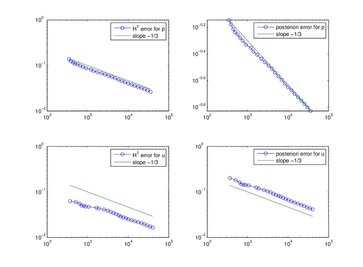
Figure 3. Example 1: Quasi-optimality of $H^{1}$- error estimates and the a posteriori error estimates.

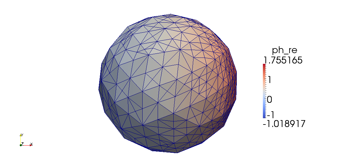
Figure 4. Example 1: An adaptive mesh with 20390 elements of $\Omega_{a}$.

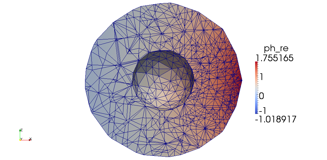
Figure 5. Example 1: The cross section of the mesh in Figure 4 on the $xz$-plane.

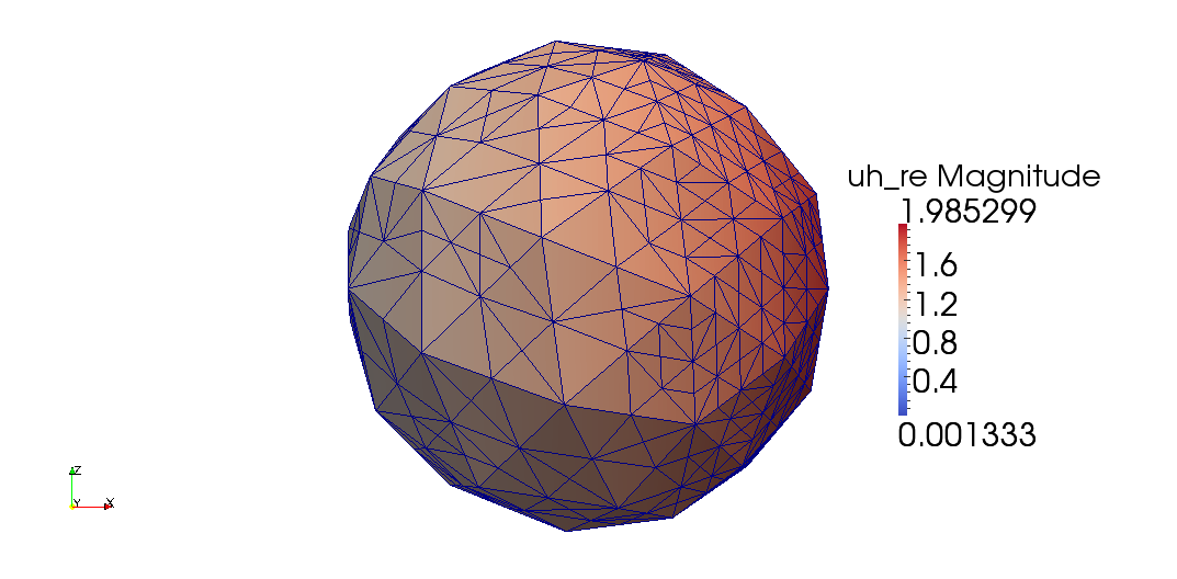
Figure 6. Example 1: An adaptive mesh with 7655 elements of $\Omega_{s}$.

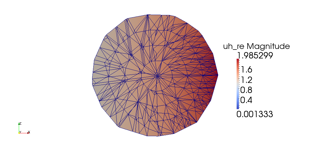
Figure 7. Example 1: The cross section of the mesh in Figure 6 on $xz$-plane.

Example 2. This example concerns the scattering of the incident plane wave

$$p^{\rm inc}(\boldsymbol{x})=e^{-{\rm i}\kappa x_{3}}.$$

The Dirichlet boundary condition on the PML layer outer boundary $\Gamma$ is set by $p=p^{\rm inc}$. We choose $\kappa=2$, $\omega=2\pi$, $\lambda=1$, $\mu=2$, and $\rho_{a}=1$. Let the elastic region and the acoustic region be $\Omega_{s}=B_{1}\backslash\bar{B}_{0}$ and $\Omega_{a}=B_{2}\backslash\bar{\Omega}_{s}$, respectively. Here $B_{0}=(-0.1,0.1)\times(-0.1,0.1)\times(-0.2,0.0),B_{1}=(-0.2,0.2)\times(-0.2,0.2)\times(-0.2,0.2)$, and $B_{2}=[-0.6,0.6]\times[-0.6,0.6]\times[-0.6,0.6]$. The PML domain is $\Omega_{\rm PML}=(0,1)\times(0,1)\times(0,1)\setminus\bar{B}_{2}$, i.e., the thickness of the PML layer is 0.4 in each direction. In this example, the elastic solid is a rectangular box with a small rectuangular dent on the surface. The solutions of $p$ and $\boldsymbol{u}$ may have singularities around the corners of the dent. We choose $\sigma=16$ and $m=2$ for the medium property to ensure the PML error is negligible compared to the finite element error.

For this example, we set the numerical solution on the very fine mesh to be a reference solution since there is no analytic solution. Figure 8 shows the errors of $p$ and $\boldsymbol{u}$ against the number of nodal points $N_{p}$ and $N_{\boldsymbol{u}}$. It is clear to note that the FEM algorithm yields a quasi-optimal convergence rate. The surface plots of the amplitude of the fields are shown as follows: Figure 9 shows the real part of $p_{h}$ for the cross section in $\Omega_{a}$ on the $yz$-plane and Figure 10 shows the real part of $\boldsymbol{u}_{h}$ for the cross section in $\Omega_{s}$ on the $yz$-plane.

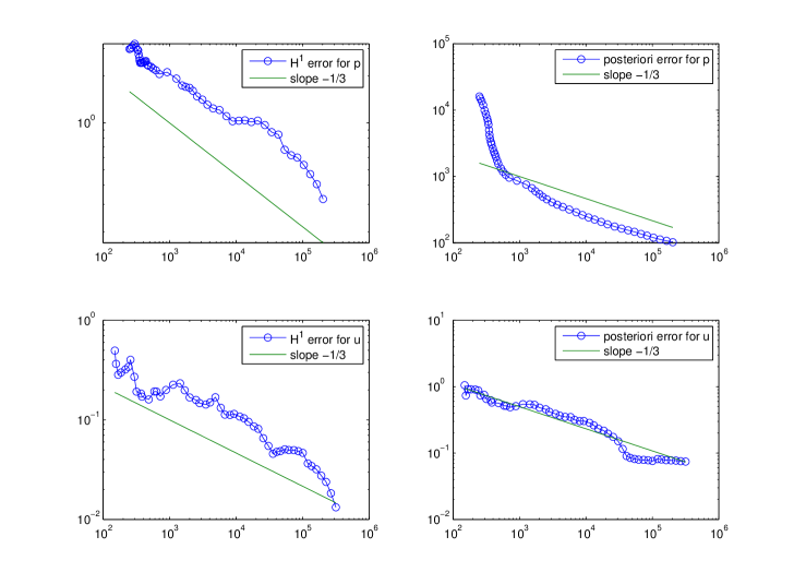
Figure 8. Example 2: Quasi-optimality of $H^{1}$- error estimates and the a posteriori error estimates.

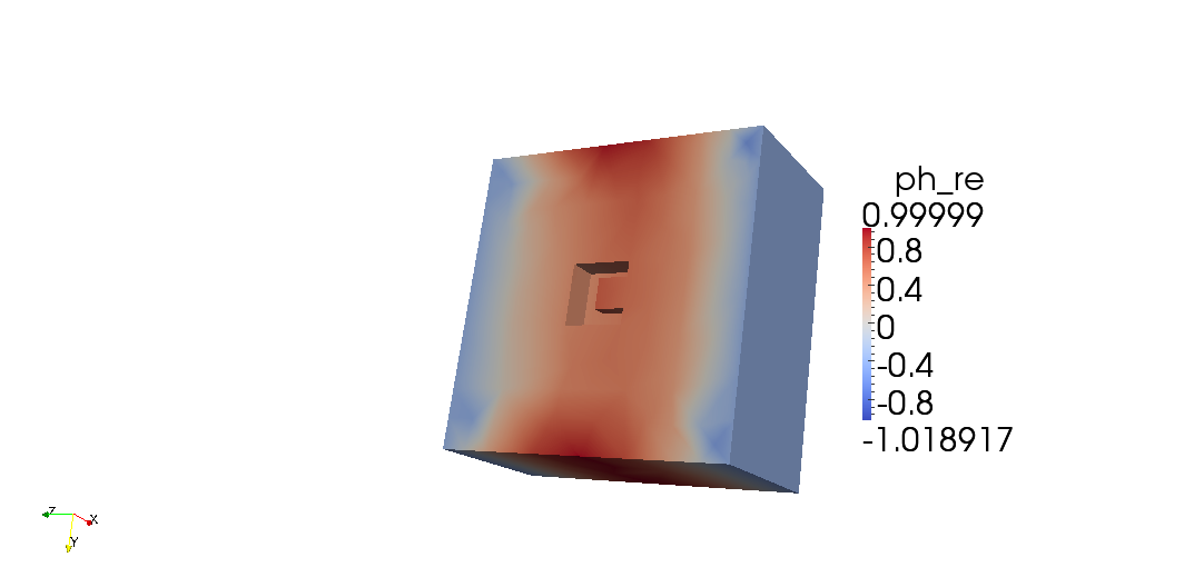
Figure 9. Example 2: The amplitude of the real part of $p_{h}$ for the cross section of $\Omega_{a}$ on the $yz$-plane.

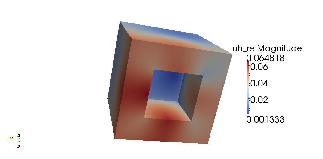
Figure 10. Example 2: The amplitude of the real part of $\boldsymbol{u}_{h}$ for the cross section of $\Omega_{s}$ on the $yz$-plane.

6. Concluding remarks

We have studied a variational formulation for the acoustic-elastic interaction problem in $\mathbb{R}^{3}$ and adopted the PML to truncate the unbounded physical domain. The scattering problem is reduced to a boundary value problem by using transparent boundary conditions. We prove that the truncated PML problem has a unique weak solution which converges exponentially to the solution of the original problem by increasing the PML parameters. We incorporate the adaptive mesh refinement with a posteriori error estimate for the finite element method to handle the problem where the solution may have singularities. Numerical results show that the proposed method is effective to solve the acoustic-elastic interaction problem.

References

- [1] I. Babuška and A. Aziz, Survey Lectures on Mathematical Foundations of the Finite Element Method, in The Mathematical Foundations of the Finite Element Method with Application to the Partial Differential Equations, ed. by A. Aziz, Academic Press, New York, 1973, 5–359.
- [2] G. Bao, P. Li, and H. Wu, An adaptive edge element method with perfectly matched absorbing layers for wave scattering by periodic structures, Math. Comp., 79 (2010), 1–34.
- [3] G. Bao and H. Wu, On the convergence of the solutions of PML equations for Maxwell’s equations, SIAM J. Numer. Anal., 43 (2005), 2121–2143.
- [4] J.-P. Bérenger, A perfectly matched layer for the absorption of electromagnetic waves, J. Comput. Phys., 114 (1994), 185–200.
- [5] J. H. Bramble and J. E. Pasciak, Analysis of a finite PML approximation for the three dimensional time-harmonic Maxwell and acoustic scattering problems, Math. Comp., 76 (2007), 597–614.
- [6] J. H. Bramble, J. E. Pasciak, and D. Trenev, Analysis of a finite PML approximation to the three dimensional elastic wave scattering problem, Math. Comp., 79 (2010), 2079–2101.
- [7] J. Chen and Z. Chen, An adaptive perfectly matched layer technique for 3-D time-harmonic electromagnetic scattering problems, Math. Comp., 77 (2008), 673–698.
- [8] Z. Chen and H. Wu, An adaptive finite element method with perfectly matched absorbing layers for the wave scattering by periodic structures, SIAM J. Numer. Anal., 41 (2003), 799–826.
- [9] Z. Chen and X. Wu, An adaptive uniaxial perfectly matched layer method for time-harmonic scattering problems, Numer. Math. Theor. Meth. Appl., 1 (2008), 113–137.
- [10] Z. Chen and X. Liu, An adptive perfectly matched layer technique for time-harmonic scattering problems, SIAM J. Numer. Anal., 43 (2005), 645–671.
- [11] Z. Chen, X. Xiang, and X. Zhang, Convergence of the PML method for elastic wave scattering problems, Math. Comp., to appear.
- [12] F. Collino and P. Monk, The perfectly matched layer in curvilinear coordinates, SIAM J. Sci. Comput., 19 (1998), 2061–1090.
- [13] F. Collino and C. Tsogka, Application of the perfectly matched absorbing layer model to the linear elastodynamic problem in anisotropic heterogeneous media, Geophysics, 66 (2001), 294–307.
- [14] D. Colton and R. Kress, Integral Equation Methods in Scattering Theory, John Wiley Sons, New York, 1983.
- [15] W. Chew and W. Weedon, A 3D perfectly matched medium for modified Maxwell’s equations with stretched coordinates, Microwave Opt. Techno. Lett., 13 (1994), 599–604.
- [16] O. V. Estorff and H. Antes, On FEM-BEM coupling for fluid-structure interaction analyses in the time domain, Internat. J. Numer. Methods Engrg., 31 (1991), 1151–1168.
- [17] B. Flemisch, M. Kaltenbacher, and B. I. Wohlmuth, Elasto-acoustic and acoustic-acoustic coupling on non-matching grids, Internat. J. Numer. Methods Engrg., 67 (2006), 1791–1810.
- [18] Y. Gao and P. Li, Time-domain analysis of an acoustic-elastic interaction problem, preprint.
- [19] Y. Gao, P. Li, and B. Zhang, Analysis of transient acoustic-elastic interaction in an unbounded structure, preprint.
- [20] F. D. Hastings, J. B. Schneider, and S. L. Broschat, Application of the perfectly matched layer (PML) absorbing boundary condition to elastic wave propagation, J. Acoust. Soc. Am., 100 (1996), 3061–3069.
- [21] T. Hohage, F. Schmidt, and L. Zschiedrich, Solving time-harmonic scattering problems based on the pole condition. II: Convergence of the PML method, SIAM J. Math. Anal., 35 (2003), 547–560.
- [22] G. C. Hsiao, On the boundary-field equation methods for fluid-structure interactions, In Problems and methods in mathematical physics (Chemnitz, 1993), vol. 134, Teubner-Texte Math., 79–88, Teubner, Stuttgart, 1994.
- [23] G. C. Hsiao, R. E. Kleinman, and L. S. Schuetz, On variational formulations of boundary value problems for fluid-solid interactions, In Elastic wave propagation (Galway, 1988), vol. 35, North-Holland Ser. Appl. Math. Mech., 321–326, North-Holland, Amsterdam, 1989.
- [24] G. C. Hsiao, T. Sánchez-Vizuet, and F.-J. Sayas, Boundary and coupled boundary-finite element methods for transient wave-structure interaction, IMA J. Numer. Anal., 37 (2017), 237–265.
- [25] X. Jiang, P. Li, J. Lv, and W. Zheng, An adaptive finite element PML method for the elastic wave scattering problem in periodic structure, preprint.
- [26] X. Jiang, P. Li, J. Lv, and W. Zheng, Convergence of the PML solution for elastic wave scattering by biperiodic structures, preprint.
- [27] M. Lassas and E. Somersalo, On the existence and convergence of the solution of PML equations, Computing, 60 (1998), 229–241.
- [28] C. J. Luke and P. A. Martin, Fluid-solid interaction: acoustic scattering by a smooth elastic obstacle, SIAM J. Appl. Math., 55 (1995), 904–922.
- [29] PHG (Parallel Hierarchical Grid), http://lsec.cc.ac.cn/phg/.
- [30] L. R. Scott and S. Zhang, Finite element interpolation of nonsmooth functions satisfying boundary conditions, Math. Comp., 54 (1990), 483–493.
- [31] D. Soares and W. Mansur, Dynamic analysis of fluid-soil-structure interaction problems by the boundary element method, J. Comput. Phys., 219 (2006), 498–512.
- [32] E. Turkel and A. Yefet, Absorbing PML boundary layers for wave-like equations, Appl. Numer. Math., 27 (1998), 533–557.