Robustness in Highly Dynamic Networks

Abstract

We investigate a special case of hereditary property that we refer to as robustness. A property is robust in a given graph if it is inherited by all connected spanning subgraphs of this graph. We motivate this definition in different contexts, showing that it plays a central role in highly dynamic networks, although the problem is defined in terms of classical (static) graph theory. In this paper, we focus on the robustness of maximal independent sets (MIS). Following the above definition, a MIS is said to be robust (RMIS) if it remains a valid MIS in all connected spanning subgraphs of the original graph. We characterize the class of graphs in which all possible MISs are robust. We show that, in these particular graphs, the problem of finding a robust MIS is local; that is, we present an RMIS algorithm using only a sublogarithmic number of rounds (in the number of nodes $n$) in the ${\cal LOCAL}$ model. On the negative side, we show that, in general graphs, the problem is not local. Precisely, we prove a $\Omega(n)$ lower bound on the number of rounds required for the nodes to decide consistently in some graphs. This result implies a separation between the RMIS problem and the MIS problem in general graphs. It also implies that any strategy in this case is asymptotically (in order) as bad as collecting all the network information at one node and solving the problem in a centralized manner. Motivated by this observation, we present a centralized algorithm that computes a robust MIS in a given graph, if one exists, and rejects otherwise. Significantly, this algorithm requires only a polynomial amount of local computation time, despite the fact that exponentially many MISs and exponentially many connected spanning subgraphs may exist.

1 Introduction

Highly dynamic networks are made of dynamic (often mobile) entities such as vehicles, drones, or robots. It is generally assumed, in these networks, that the set of entities (nodes) is constant, while the set of communication links varies over time. Many classical assumptions do not hold in these networks. For example, the topology may be disconnected at any instant. It may also happen that an edge present at some time never appears again in the future. In fact, of all the edges that appear at least once, one can distinguish between two essential sets: the set of recurrent edges, which always reappear in the future (or remain present), and the set of non recurrent edges which eventually disappear in the future. The static graph containing the union of both edge sets is called the footprint of the network [7], and its restriction to the recurrent edges is the eventual footprint of the network [5].

It is not clear, at first, what assumptions seem reasonable in a highly dynamic network. Special cases have been considered recently, such as always-connected dynamic networks [20], $T$-interval connected networks [14], or networks the edges of which correspond to pairwise interactions obeying a uniform random scheduler (see e.g. [2, 17]). Arguably, one of the weakest possible assumption is that any pair of nodes be able to communicate infinitely often through temporal paths (or journeys). Interestingly enough, this property was identified more than three decades ago by Awerbuch and Even [3] and remained essentially ignored afterwards. The corresponding class of dynamic networks (Class 5 in [7]—here referred to as ${\cal TC^{\cal R}}$ for consistency with various notations [8, 12, 1]) is however one of the most general and it actually includes the three aforementioned cases.

Dubois et al. [8] observe that class ${{\cal TC^{\cal R}}}$ is actually the set of dynamic networks whose eventual footprint is connected. In other words, it is more than reasonable to assume that some of the edges are recurrent and their union does form a connected spanning subgraph. Solving classical problems such as symmetry-breaking tasks relative to this particular set thus makes sense, as the nodes can rely forever on the corresponding solution, even though intermittently [6, 8]. Unfortunately, it is impossible for a node to distinguish between the set of recurrent edges and the set of non recurrent edges. So, the best the nodes can do is to compute a solution relative to the footprint, hoping that this solution still makes sense in the eventual footprint, whatever it is. (Whether, and how the nodes can learn the footprint itself is discussed later on.)

This context suggests a particular form of heredity which we call robustness. In classical terms, robustness can be formulated as the fact that a given property must be inherited by all the connected spanning subgraphs of the original graph. Significantly, this concept admits several possible interpretations, including the dynamic interpretation developed here. A more conventional, almost direct interpretation is that some edges in a classical (static) network are subject to permanent failure at some point, and the network is to be operated so long as it remains connected. While this interpretation is more intuitive and familiar, we insist on the fact that the dynamic interpretation of robustness is what makes its study compelling, for this notion arises naturally in class ${\cal TC^{\cal R}}$, which is one of the most general class of dynamic networks imaginable. The reader may adopt either interpretation while going through the paper, keeping in mind that our results apply to both contexts and are therefore quite general.

Contributions. We investigate the concept of robustness of a property, with a focus on the maximal independent set (MIS) problem, which consists of selecting a subset of nodes none of which are neighbors (independence) and such that no further node can be added to it (maximality). As it turns out, a robust MIS may or may not exist, and if it exists, it may or may not be computable locally depending on the considered graph (resp. footprint).

(a)

(b)

(c)

(d)

Figure 1: Four examples of MISs in various graphs (resp. footprints).

For example, if the graph is a triangle (see Figure 1a), then only one MIS exists up to isomorphism, consisting of a single node. However, this set is no longer maximal in one of the possible connected spanning subgraphs (e.g. after removing an adjacent edge to the selected node). Therefore, the triangle graph admits no robust MIS. Some graphs do admit a robust MIS, but not all of the MISs are robust. Figures 1b and 1c show two MISs in the bull graph, only one of which is robust. Finally, some graphs like the square graph (Figure 1d) are such that all MISs are robust. Although the last two examples seem to suggest that robust MISs are related to maximum MISs, being maximum is actually neither a necessary nor a sufficient condition.

In this paper, we characterize the class of graphs such that all MISs are robust, denoted ${\cal RMIS^{\forall}}$. We prove that ${\cal RMIS^{\forall}}$ consists exactly of the union of complete bipartite graphs and a new class of graphs called sputniks, which contains among others all the trees (for which any property is trivially robust). While the sufficient side is easy to establish, proving that these graphs are the only ones is more difficult. Interestingly, while the best known algorithms for deterministic distributed MIS in general graphs are superlogarithmic in the number of nodes $n$, namely they take $2^{\mathcal{O}(\sqrt{\log n})}$ rounds [21] (better randomized algorithms are known [15]), graphs in ${\cal RMIS^{\forall}}$ turn out to be specific enough to find an MIS (robust by definition) by using only information available within a sublogarithmic distance. We present an algorithm that first settles specific subsets of the networks using information available within constant distance, the residual instance being a disjoint union of trees. The residual instance can then be given to state-of-the-art algorithms like Barenboim and Elkin’s for graphs of bounded arboricity [4], which is known to use only information within distance $\mathcal{O}(\log n/\log\log n)$. An added benefit of this reduction is that any further progress on the MIS problem on trees will automatically transpose to robust MISs in ${\cal RMIS^{\forall}}$. (Note that we deliberately do not use the terms “rounds” or “time”, due to the non equivalence of locality and time in the context of a footprint.)

Next, we turn our attention to general graphs and ask whether a robust MIS can be found (if one exists) using only local information. We answer negatively, proving an $\Omega(n)$ lower bound on the locality of the problem. This result implies a separation between the MIS problem and the robust MIS problem in general graphs, since the former is feasible within $2^{\mathcal{O}(\sqrt{\log n})}$ hops [21]. It also implies that no strategy is essentially better than collecting the network at a single node and subsequently solving the problem in an offline manner. Motivated by this observation, we consider the offline problem of finding a robust MIS in a given graph if one exists (and rejecting otherwise). The trivial strategy amounts to enumerating all MISs until a robust one is found, however there may be exponentially many MISs in general graphs (Moon and Moser [18], see also [10, 11] for an extension to the case of connected graphs). We present a polynomial time algorithm for computing a robust MIS in any given graph (if one exists). Our algorithm relies on a particular decomposition of the graph into a tree of biconnected components (${\cal ABC}$-tree), along which constraints are propagated about the MIS status of special nodes in between the components. The inner constraints of non trivial components are solved by reduction to the 2-SAT problem (which is tractable). As a by-product, the set of instances for which a robust MIS is found characterizes the existential analogue of ${\cal RMIS^{\forall}}$, that is the class ${\cal RMIS^{\exists}}$ of all graphs that admit a robust MIS. (Whether a closer characterization exists is left as an open question.)

Further discussion on the dynamic interpretation. As pointed out, in a dynamic network there is no way to distinguish between recurrent and non recurrent edges, therefore the nodes cannot learn the eventual footprint [5] (this observation is the very basis of the notion of robustness). Now, what about the union of both types of edges, that is, the footprint itself? Clearly, the footprint can never be decided in a definitive sense by the nodes, since some edges may appear arbitrary late for the first time. However, it is also clear that every edge of the footprint will eventually appear; thus, over time the nodes can learn the footprint in a stabilized way, by updating their representation as new edges are detected. It is therefore possible to update some structure or property that eventually relates to the correct footprint. (Alternatively, one may assume simply that prior information about the footprint is given to the nodes, or that an oracle informs the nodes once every edge of the footprint has appeared.) Again, the reader is free to ignore the dynamic interpretation if the static one makes for a sufficient motivation.

Outline. Section 2 presents the main definitions and concepts. Then, we characterize in Section 3 the class ${\cal RMIS^{\forall}}$ and present a dedicated MIS algorithm that requires only information up to a sublogarithmic number of hops. Section 4 establishes the non-locality of the problem in general and describes a tractable algorithm that computes a robust MIS in a given graph if one exists. Section 5 concludes with some remarks.

2 Main concepts and definitions

Many of the concepts presented in the introduction, including that of temporal paths, footprint, or classes of dynamic networks are not defined here. The authors believe that the informal descriptions given in introduction are sufficient to understand the dynamic interpretation of the results. (If that is not the case, the reader is referred to [7] for thorough definitions using the time-varying graph formalism.) Our results themselves are formulated using standard concepts of graph theory, making them independent from both interpretations.

2.1 Basic definitions

Let $G=(V,E)$ be an undirected graph, with $V$ the set of nodes (vertices) and $E$ the set of bidirectional communication links (edges). We denote by $n=|V|$ the number of nodes in the graph, and by $D$ the diameter of the graph, that is, the length of the longest shortest path in $G$ over all possible pairs of nodes. We denote by $N(v)$ the neighborhood of a vertex $v$, which is the set of vertices $\{w:\{v,w\}\in E\}$. The degree of a vertex $v$ is $|N(v)|$. A vertex is pendant if it has degree $1$. A cut vertex (or articulation point) is a vertex whose removal disconnects the graph. A cut edge (or bridge) is an edge whose removal disconnects the graph. We say that an edge is removable if it is not a cut edge. A spanning connected subgraph of a graph $G=(V_{G},E_{G})$ is a graph $H=(V_{H},E_{H})$ such that $V_{H}=V_{G}$, $E_{H}\subseteq E_{G}$, and $H$ is connected. In the most general variant, we define robustness as follows.

Definition 1 (Robustness).

A property $P$ is said to be robust in $G$ if and only if it is satisfied in every connected spanning subgraph of $G$ (including $G$ itself).

In other words, a robust property holds even after an arbitrary number of edges are removed without disconnecting the graph. Robustness is a special case of hereditary property, and more precisely a special case of decreasing monotone property (see for instance [13]). In this paper, we focus on the maximal independent set (MIS) problem. An MIS is a set of nodes such that no two nodes in the set are neighbors and the set is maximal for the inclusion relation. Following Definition 1, a robust MIS in a graph $G$ (RMIS, for short) is an MIS that remains maximal and independent in every connected spanning subgraph of $G$. Observe that independence is stable under the removal of edges; therefore, it is sufficient that the MIS be maximal in all these subgraphs in order to be an RMIS. We define two classes of graphs related to the robustness of MISs.

Definition 2 (${\cal RMIS^{\forall}}$).

This class is the set of all graphs in which all MISs are robust.

Definition 3 (${\cal RMIS^{\exists}}$).

This class is the set of all graphs that admit at least one robust MIS.

We define the distributed problem of computing an RMIS in a given graph as follows.

Definition 4 (RobustMIS problem).

Given a graph $G$ and an algorithm ${\cal A}$ executed at every node of $G$, ${\cal A}$ solves RobustMIS on $G$ iff every node eventually terminates by outputting IN or OUT, and the set of nodes outputting IN forms an RMIS on $G$. Algorithm ${\cal A}$ solves RobustMIS in a class of graphs ${\cal C}$ iff for all $G\in{\cal C}$, ${\cal A}$ solves RobustMIS on $G$.

Finally, let us define two classes of graphs that turn out to be closely related to RMISs, namely complete bipartite graphs and sputnik graphs. The latter is introduced here for the first time.

Definition 5 (Complete bipartite graph).

A complete bipartite graph is a graph $G=(V_{1}\cup V_{2},E)$ such that $V_{1}\cap V_{2}=\emptyset$ and $E=V_{1}\times V_{2}$. In words, the vertices can be partitioned into two sets $V_{1}$ and $V_{2}$ such that every vertex in $V_{1}$ shares an edge with every vertex in $V_{2}$ (completeness), and these are the only edges (bipartiteness).

Definition 6 (Sputnik).

A graph is a sputnik iff every vertex belonging to a cycle also has a pendant neighbor. (An example of sputnik is shown in Figure 2.)

2.2 Computational model

Based on the chosen interpretation of our results, the base graph in the above definitions refers either to the footprint of a dynamic network, or to the network itself. In the dynamic case, the actual timing of the edges is arbitrary, so the classical equivalence between time and locality in synchronous network does not hold. Nonetheless, we rely on the ${\cal LOCAL}$ model [16, 19] to describe the algorithms. To avoid confusion between locality and time in the dynamic case, we always state the complexities in terms of locality, saying that an algorithm (or problem) is $\mathcal{O}(f(G))$-local if it can be solved in $\mathcal{O}(f(G))$ rounds in the ${\cal LOCAL}$ model. (Other terminologies include saying that such problems are in $LD(f(G))$ [9].) For completeness, let us recall the main features of the $\mathcal{LOCAL}$ model. In this model, the nodes operate in synchronous discrete rounds and they wake up simultaneously. In each round, a node can exchange messages of arbitrary size with its neighbors and perform some local (typically unrestricted) computation. The complexity of an algorithm over a class of graphs is the maximum number of rounds, taken over all graphs of this class, performed until all nodes have terminated. In the dynamic interpretation of our results, the algorithms are seen as being restarted every time the local knowledge of the footprint changes.

3 Characterization of ${\cal RMIS^{\forall}}$ and locality of RobustMIS

In this section, we show that ${\cal RMIS^{\forall}}$, the class of graphs in which all MISs are robust, corresponds exactly to the union of complete bipartite graphs and sputnik graphs. Then we present an algorithm that solves RobustMIS in ${\cal RMIS^{\forall}}$ using information available only within a sublogarithmic number of hops in $n$.

3.1 Characterization of ${\cal RMIS^{\forall}}$

We first show that all MISs are robust in complete bipartite graphs and in sputnik graphs. Due to space limitation, the proofs of the two following lemmas are postponed to Appendix A. They follow easily from the very definition of RMIS and of these classes of graphs.

Lemma 1.

All MISs are robust in complete bipartite graphs.

Lemma 2.

All MISs are robust in sputnik graphs.

We now prove the stronger result that if a graph is such that all possible MISs are robust, then it must be either a bipartite complete graph or a sputnik.

Lemma 3.

If $G$ is not a sputnik, and yet every MIS in $G$ is robust, then $G$ is bipartite complete.

Proof.

If $G$ is not a sputnik, then some node $u$ in a cycle $C\subseteq G$ has no pendant neighbor. In general, $u$ may be an articulation point, and so the graph $G\setminus\{u\}$ may result in several components. Let $X_{1},X_{2},\dots$ be the resulting components with vertex $u$ back in each of them. In particular, let $X_{1}$ be the one that contains $C$ and observe that $X_{1}$ contains at least $3$ vertices (cycle). The other components, if they exist, all contain at least two vertices other than $u$ (otherwise $u$ would have a pendant neighbor).

Claim 1: If all MISs in $G$ are robust, then all neighbors of $u$ in $X_{1}$ have the same neighborhood.

We prove this claim by contradiction. Let two neighbors $v_{1},v_{2}$ of $u$ be such that $N(v_{1})\neq N(v_{2})$. We will show that at least one MIS is not robust. Without loss of generality, assume that some vertex $x$ belongs to $N(v_{1})\setminus N(v_{2})$. Then we can build an MIS that contains both $v_{2}$ and $x$ (as a special case, $x$ may be the same vertex as $v_{2}$, but this is not a problem). For each of the components $X_{i\geq 2}$, choose an edge $\{u,w_{i}\}\in X_{i}$ and add another neighbor of $w_{i}$ to the MIS (such a neighbor exists, as we have already seen). One can see that $u$, $v_{1}$ and all $w_{i}$ can no longer enter the MIS because they all have neighbors in it. Now, choose the remaining elements of the MIS arbitrarily. We will show that the resulting MIS is not robust, by consider the removal of edges as follows. In all components $X_{i\geq 2}$, remove all edges incident to $u$ except $\{u,w_{i}\}$; and in $X_{1}$, remove all edges incident to $u$ except $\{u,v_{1}\}$. The resulting graph remains connected, by definition, since each of the $X_{i}\setminus\{u\}$ is connected. And yet, $u$ no longer has a neighbor in the MIS, which contradicts robustness. $\blacksquare$

Now, Claim 1 implies that none of $u$’s neighbors in $X_{1}$ has a pendant neighbor (since their neighborhoods are the same). As a result, the arguments that applied to $u$ because of its absence of pendant neighbors, apply in turn to $u$’s neighbors in $X_{1}$. In particular, it means that if some node $v$ is neighbor to $u$ in $X_{1}$, then all neighbors of $v$ (including $u$) must have the same neighborhood. Therefore, $u$ cannot be an articulation point and we are left with the single component $X_{1}$, in which all neighbors of $u$ have the same neighbors and these neighbors in turn have the same neighbors, which implies that the graph is complete bipartite. ∎

Based on Lemmas 1, 2, and 3, we conclude with the following theorem.

Theorem 1.

All MISs are robust in a graph $G$ if and only if $G$ is complete bipartite or sputnik.

3.2 RobustMIS is locally solvable in ${\cal RMIS^{\forall}}$

Figure 2: A sputnik and its sets $P$ (dotted set), $N$ (dashed set), and $F$ (plain set).

We now prove that computing deterministically an RMIS in class ${\cal RMIS^{\forall}}$ can be done locally, by presenting a distributed algorithm that computes a (regular) MIS using only information available within $o(\log n)$-hops a sublogarithmic number of hops in $n$. By definition of the class, this MIS is robust. Informally, the algorithm proceeds as follows (due to space limitations, the pseudo-code and the formal proof of the algorithm are moved to Appendix A). Class ${\cal RMIS^{\forall}}$ consists of exactly the union of bipartite complete graphs and sputniks (Theorem 1). First, the nodes decide if the graph is complete bipartite by looking within a constant number of hops (three). If so, membership to the MIS is decided according to some convention (e.g. all nodes in the same part as the smallest identifier are in the MIS). Otherwise, the graph must be a sputnik and every node decides (without more information) which of the following three cases it falls into: 1) it is a pendant node (set $P$ in Figure 2), 2) it is not a pendant node but has at least one pendant neighbor (set $N$), or 3) none of the two cases apply (set $F$). In the first case, it enters the MIS, while in the second it decides not to. We prove that the set of nodes falling into the third case does form a disjoint union of trees, each of which can consequently be solved by state-of-the-art algorithms. In particular, Barenboim and Elkin [4] present a $\mathcal{O}(\log n/\log\log n)$-local algorithm that solves MIS in graphs of bounded arboricity (and a fortiori trees). On the negative side, we show (using standard arguments) that Linial’s $\Omega(\log^{*}n)$ lower bound for $3$-coloring [16] in cycles extends to RobustMIS in class ${\cal RMIS^{\forall}}$, leading to the following theorem.

Theorem 2.

RobustMIS is $\Omega(\log^{*}n)\cap\mathcal{O}(\log n/\log\log n)$-local in class ${\cal RMIS^{\forall}}$.

4 Nonlocality of RobustMIS in general graphs and global resolution

In this section, we prove that the problem of computing deterministically an RMIS in general graphs, if one exists, is not local. Precisely, we first observe that deciding whether an RMIS exists is not a local problem; then, we prove a $\Omega(n)$ lower bound on the distance at which it might be necessary to look to solve the problem if an RMIS exists, where $n$ is the diameter of the network. Motivated by this result, we present an offline algorithm that compute an RMIS, in polynomial time, if one exists. It can be used in a strategy where all the information about the network is collected at one node (or several, the algorithm being deterministic).

Figure 3: The graph $G_{k}$ ($k\in\mathbb{N}$) and one of its two possible robust MISs.

4.1 RobustMIS is non local in general graphs

Let us first observe that the problem of deciding whether an RMIS exists is not local. Consider two graphs $G_{1}$ and $G_{2}$ which respectively consist of a $\mathcal{O}(n)$-long path and to a lollipop graph (i.e. a graph joining a $\mathcal{O}(n)$-long path to a clique of size $\mathcal{O}(n)$). Then, clearly, a node at one extremity of $G_{1}$ and the (unique) pendant node of $G_{2}$ cannot distinguish their $o(n)$ neighborhood (even with identifiers, which could be exactly the same in this neighborhood) whereas $G_{1}$ admits an RMIS and $G_{2}$ does not. We go further and prove that, even if some RMISs do exist, then finding one is non local. To prove this result, we exhibit an infinite family of graphs $(G_{k})_{k\in\mathbb{N}}$, each of which has diameter linear in $k$ (and $n$). We first show through Lemmas 4 and 5 that every $G_{k}$ admits only two RMISs $M_{1}$ and $M_{2}$ which are complements of each other; that is $M_{2}=\overline{M_{1}}=V\setminus M_{1}$. Intuitively, these MISs are such that two nodes at distance $\mathcal{O}(n)$ must take opposite decisions, although they have the same view up to distance $\mathcal{O}(n)$. (The real proof is more complex and involves showing that identifiers do not help either.) As a result, the nodes may have to collect information up to distance $\Omega(n)$ in order to decide consistently.

Let $(G_{k})_{k\in\mathbb{N}}$ be an infinite famility of graphs defined as follows. Graph $G_{0}=(V_{0},E_{0})$ is such that $V_{0}=\{a_{0},b_{0},c_{0},\alpha_{0},\beta_{0},\gamma_{0}\}$ and $E_{0}$ induces a cycle $a_{0}$-$b_{0}$-$c_{0}$-$\gamma_{0}$-$\beta_{0}$-$\alpha_{0}$-$a_{0}$ as shown in Figure 3. Then $G_{k}=(V_{k},E_{k})$ is obtained from $G_{k-1}=(V_{k-1},E_{k-1})$ as follows: $V_{k}=V_{k-1}\cup\{a_{k},b_{k},c_{k},\alpha_{k},\beta_{k},\gamma_{k}\}$ and $E_{k}=E_{k-1}\cup\{\{\beta_{k-1},\alpha_{k}\},\{\beta_{k-1},\gamma_{k}\},$ $\{\alpha_{k},\beta_{k}\},\{\gamma_{k},\beta_{k}\},\{b_{k-1},a_{k}\},\{b_{k-1},c_{k}\},\{a_{k},b_{k}\},\{c_{k},b_{k}\}\}$.

For any $k$, define $M_{1}$ as the set of nodes $\{\alpha_{i},\gamma_{i},b_{i}|i\leq k\}$ and $M_{2}=\{a_{i},c_{i},\beta_{i}|i\leq k\}$. Observe that $M_{2}=V_{k}\setminus M_{1}$ (written $\overline{M_{1}}$). Set $M_{1}$ is illustrated in Figure 3.

Lemma 4.

For any $k\geq 0$, $M_{1}$ and $M_{2}$ are RMISs in $G_{k}$.

Proof.

We prove this for $M_{1}$. The same holds symmetrically for $M_{2}$. First, observe that $M_{1}$ is a valid MIS: no two of its nodes are neighbors by construction (independence) and all nodes in $V_{k}\setminus M_{1}$ have neighbors in $M_{1}$ (maximality). Now, to obtain a connected spanning subgraph of $G_{k}$, one can remove from $E_{k}$ at most one edge from each simple cycle of $G_{k}$. Since any node of $V_{k}\setminus M_{1}$ has a number of neighbors in $M_{1}$ strictly greater than the number of simple cycles it belongs to, $M_{1}$ is robust. ∎

Lemma 5.

For any $k\geq 0$, $M_{1}$ and $M_{2}$ are the only two RMISs in $G_{k}$, implying that nodes $b_{k}$ and $\beta_{k}$ must take opposite decisions in all RMISs.

Proof.

We say that an edge $e\in E$ is critical with respect to some MIS $M$ in $G_{k}$ if $e$ is removable (i.e. not a cut edge) and $M$ is no longer maximal in $(V_{k},E_{k}\setminus\{e\})$. The existence of a critical edge implies that the considered MIS is not robust. Let us now consider an RMIS $M$ in $G_{k}$. We prove several claims on $M$.

Claim 1: If $\alpha_{0}\in M$, then $\{\gamma_{0},b_{0}\}\subseteq M$ and $\{\beta_{0},c_{0},a_{0}\}\subseteq\overline{M}$.

If $\alpha_{0}\in M$, then $\{\beta_{0},a_{0}\}\subseteq\overline{M}$ (independence). It also holds that $b_{0}\in M$, otherwise the edge $\{\alpha_{0},a_{0}\}$ is critical (robustness). It follows that $c_{0}\notin M$ (independence) and $\gamma_{0}\in M$ (maximality).

Claim 2: If $\alpha_{0}\notin M$, then $\{\gamma_{0},b_{0}\}\subseteq\overline{M}$ and $\{\beta_{0},c_{0},a_{0}\}\subseteq M$. (symmetric to Claim 1)

Claim 3: If $\alpha_{0}\in M$, then $\{\alpha_{i},\gamma_{i}\}\subseteq M$ and $\beta_{i}\notin M$ for all $i\leq k$.

By contradiction, if $\beta_{i}\in M$ for some $i$, then $\{\alpha_{i},\gamma_{i}\}\subseteq\overline{M}$ (independence). Let $i$ be smallest possible, then edges $\{\alpha_{i},\beta_{i}\}$ and $\{\beta_{i},\gamma_{i}\}$ are critical w.r.t. $M$ (recall that, if $i>0$, $\beta_{i-1}\notin M$ by construction and $\beta_{0}\notin M$ by Claim 1), which contradicts robustness. Therefore, $\beta_{i}\notin M$. The maximality of $M$ allows us to conclude.

Claim 4: If $\alpha_{0}\notin M$, then $\{\alpha_{i},\gamma_{i}\}\subseteq\overline{M}$ and $\beta_{i}\in M$ for all $i\leq k$. (symmetric to Claim 3)

Claim 5: If $\alpha_{0}\in M$, then $\{a_{i},c_{i}\}\subseteq\overline{M}$ and $b_{i}\in M$ for all $i\leq k$.

By contradiction, if $b_{i}\notin M$ for some $i$, then $\{a_{i},c_{i}\}\subseteq\overline{M}$ (independence). Let $i$ be smallest possible (recall that, if $i>0$, $b_{i-1}\in M$ by construction and $b_{0}\in M$ by Claim 1). Let $w$ be $b_{0}$ if $i=0$ and be $b_{i-1}$ otherwise. The edges $\{w,a_{i}\}$ and $\{w,\gamma_{i}\}$ are then critical, which contradicts robustness. Therefore, $b_{i}\in M$. The independence of $M$ allows us to conclude.

Claim 6: If $\alpha_{0}\notin M$, then $\{a_{i},c_{i}\}\subseteq M$ and $b_{i}\notin M$ for all $i\leq k$. (symmetric to Claim 5)

Claims 1 to 6 imply that $M=M_{1}$ if $\alpha_{0}\in M$ and $M=M_{2}$ otherwise. ∎

Finally, we relate these results to the locality of the RobustMIS problem.

Theorem 3.

RobustMIS requires the nodes to use information up to distance $\Omega(n)$ in $G_{k}$.

Proof.

The proof would be straightforward in an anonymous network, due to the fact that $b_{k}$ and $\beta_{k}$ have indistinguishable structural neighborhoods (a.k.a. views [22]) up to distance $\mathcal{O}(n)$, and yet, they must take different decisions (Lemma 5). Unique identifiers make the argument more complicated, since $b_{k}$ and $\beta_{k}$ do have unique labeled views (i.e. views taking into account identifiers) even at distance $0$.

Let us call $b_{k}$ and $\beta_{k}$ the extremities of the network. Observe that the distance between both extremities is larger than $4k$. Let ${\cal L}_{1}$, ${\cal L}_{2}$, and ${\cal L}_{3}$ be three possible labeling functions that assign unique identifiers to the neighborhood of an extremity up to distance $k$ (say) and such that the three labelings have no identifier in common. Let $G_{k}^{1}$ be the labeled graph whose structure is isomorphic to $G_{k}$, in which the neighborhood of $b_{k}$ is labeled according to ${\cal L}_{1}$ and the neighborhood of $\beta_{k}$ is labeled according to ${\cal L}_{2}$; the rest of the nodes are labeled arbitrarily. Let $G_{k}^{2}$ be defined similarly, but using ${\cal L}_{3}$ instead of ${\cal L}_{2}$ in the neighborhood of $\beta_{k}$. Finally, let $G_{k}^{3}$ be defined similarly, but using ${\cal L}_{2}$ in the neighborhood of $b_{k}$ and ${\cal L}_{3}$ in the neighborhood of $\beta_{k}$. Now, if $b_{k}$ and $\beta_{k}$ use only information up to distance $k$, then they must take identical decisions in at least one of the three labeled graphs, contradicting Lemma 5. ∎

4.2 A global algorithm to compute a robust MIS (if one exists)

We now describe an algorithm that tests constructively whether an RMIS exists in a graph $G$. Our algorithm relies on the construction of an auxiliary tree called $\mathcal{ABC}$-tree, which represents a particular decomposition of the graph based on biconnected components (it is neither a block-cut tree, nor a bridge tree, but a mix of these two types of decomposition). Roughly speaking, our algorithm works by propagating constraints about the MIS along the $\mathcal{ABC}$-tree. Each non-trivial component is solved on the way up by means of a reduction of its constraints to 2-SAT (which is polynomial-time solvable).

In the following, we describe how the $\mathcal{ABC}$-tree is built over $G$. It is followed by an informal presentation of the algorithm—due to the lack of space, the formal algorithm has been moved to Appendix B and its proof is presented in Appendix C.

Decomposition of $G$. In the context of this section, we call biconnected component (or simply component) in $G$ a maximal subgraph $H\subseteq G$ such that the removal of any node in $H$ does not disconnect $H$ (i.e. $H$ is $2$-vertex-connected). By abuse of notation, we write $u\in H$ if $u$ is a vertex of the subgraph $H$. We consider here a mix of the so-called block-cut tree and bridge tree and refer to it as the $\mathcal{ABC}$-tree. Let $\mathcal{S}$ be the set of biconnected components of $G$ (see Figure 4 for an illustration).

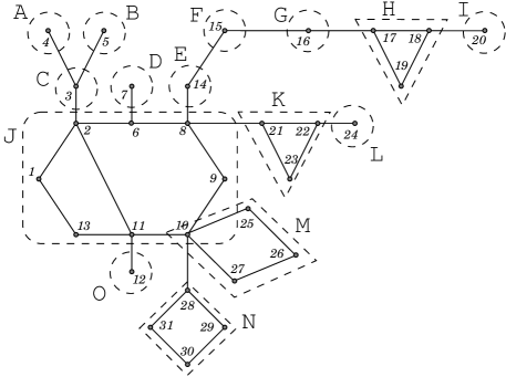
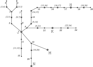
Figure 4: Decomposition of a graph into biconnected components (left) and the corresponding $\mathcal{ABC}$-tree (right). Nodes with shapes $\circ$ and $\Diamond$ correspond respectively to pendant vertices ($\in\mathcal{P}$) and articulation points ($\in\mathcal{A}$). Nodes with shape $\Box$ correspond to bridge edges ($\in\mathcal{B}$), and nodes with shape $\bigcirc$ show components that contain at least $3$ vertices ($\in\mathcal{C}$).

Two adjacent components either share a common articulation point or they are linked by a bridge. For instance, node $10$ in Figure 4 is common to components $J$ and $M$, and edges $\{6,7\}$ and $\{8,21\}$ are bridges between $D$ and $J$, and $J$ and $K$ respectively. Let $\mathcal{A}$ be the set of all articulation points (whether or not they are shared) and $\mathcal{B}$ the set of bridges. Let $\mathcal{P}$ be the set of all pendant vertices, which form singleton components—in Figure 4, $\mathcal{P}=\{4,5,7,12,20,24\}$. Finally, let $\mathcal{C}$ be the set of components that contain three or more vertices—$\mathcal{C}=\{H,J,K,M,N\}$. Remark that if $\mathcal{C}$ is empty, then $G$ is acyclic.

The ${\cal ABC}$ decomposition (or $\mathcal{ABC}$-tree) of $G$, is the graph ${\cal T}_{G}=(V^{\prime},E^{\prime})$ such that $V^{\prime}=\mathcal{A}\cup\mathcal{B}\cup\mathcal{C}\cup\mathcal{P}$ and $E^{\prime}$ is defined by the two following rules: $(i)$ $\forall a\in\mathcal{A}$, $\forall c\in\mathcal{C}$, $\{a,c\}\in E^{\prime}$ if and only if $a\in c$; and $(ii)$ $\forall b=\{u,v\}\in\mathcal{B}$, $\{b,u\}\in E^{\prime}$ and $\{b,v\}\in E^{\prime}$. Figure 4 (right side) shows the $\mathcal{ABC}$-tree corresponding to the graph of the left side.

Algorithm. The algorithm works on ${\cal T}_{G}$, the $\mathcal{ABC}$-tree made over the four sets $\mathcal{A}$, $\mathcal{B}$, $\mathcal{C}$, and $\mathcal{P}$ with respect to $G$. If the set $\mathcal{C}$ is empty, it means that $G$ is acyclic. In that case, $G$ trivially admits an RMIS, which is returned by the algorithm. Otherwise ($\mathcal{C}\neq\emptyset$), a component vertex $C\in\mathcal{C}$ is arbitrarily selected to be the root of ${\cal T}_{G}$, denoted by $\mathcal{R_{{\cal T}_{G}}}$. Then, the classical concepts in oriented trees, such as children, parent, descendant, subtree, or leaf apply to the vertices of ${\cal T}_{G}$. For ease of reading, we abuse the term “admit” by saying that a subtree $\hat{T}$ of ${\cal T}_{G}$ “admits an RMIS” if the subgraph of $G$ corresponding to $\hat{T}$ admits an RMIS.

At the higher level, the algorithm proceeds within two phases. Based on ${\cal T}_{G}$, the first one is called the labeling phase. Initiated from the leaves of the tree, it evaluates whether the subgraph of $G$ corresponding to the current subtree admits a robust MIS or not and labels each subtree according to that. If it does admit an RMIS, it may impose some constraints about the membership of the higher nodes. For instance, a robust MIS of the subtree may exist only if the articulation point leading up to the parent belongs to it. Then, the goal of the labeling phase consists of propagating (and memorizing within labels) such constraints up through subtle interactions among the various types of vertices (namely, pendant nodes, articulation point, bridge, or component) leading up to the root. Besides, the inner topological configuration of a single component may also impose non-trivial constraints for the existence of a robust MIS. Intuitively, it must have properties that relate to (but are slightly more complex than) bipartiteness. The second (short) phase of the algorithm is called the deciding phase. It simply consists of deciding whether the graph admits a robust MIS or not considering the label of the root of the $\mathcal{ABC}$-tree.

Labeling Phase. As already mentioned, a given subtree $\hat{T}$ of ${\cal T}_{G}$ may or may not admit an RMIS. Intuitively, the global decision depends on topological contraints, established over $\hat{T}$. Obviously, those constraints influence the possible topological organization of a global RMIS toward the parent of $\hat{T}$. So, this mecanism involves in a crucial way the unique $x\in\hat{T}$ such that $x\in\mathcal{A}\cup\mathcal{P}$ through which $\hat{T}$ is connected to the remainder of ${\cal T}_{G}$. In the following $x$ is called the attachment point of $\hat{T}$. In other words and more conveniently, the attachment point of the root $r$ of $\hat{T}$ is either $r$ itself if $r\in\mathcal{A}\cup\mathcal{P}$ or the parent of $r$ if $r\in\mathcal{B}\cup\mathcal{C}$. For instance, in Figure 4, assuming that $\mathcal{R_{{\cal T}_{G}}}$ is the component vertex M, then, $4$ is the attachment point of itself ($4\in\mathcal{P}$), $8$ is the one of both $\{8,14\}$ and $\{8,21\}$, while $10$ is the attachment point of $\{10,28\}$ ($\in\mathcal{B}$), $M$ ($\in\mathcal{C}$), and itself ($\in\mathcal{A})$.

Constraint transmission takes place from the leaves to the root by tagging each vertices with the following labels: PI for Possibly In (meaning that $\hat{T}$ admits an RMIS that includes $x$, the attachment point of $\hat{T}$); PO for Possibly Out (meaning that $\hat{T}$ admits an RMIS that does not include $x$); PE for Possibly External (meaning that $\hat{T}$ is not tagged PO, and it admits an RMIS that does not include $x$ assuming that another node $x^{\prime}$, external to $\hat{T}$ belongs to the RMIS); and N for Negative (meaning that none of the three other tags is applicable to $\hat{T}$). An extra label, E is used at the root (see below). Note that the algorithm associates to each label a set of vertices that is used to store a robust MIS of $\hat{T}$ satisfying the constraint of the label. Also, remark that PO and PE are mutually exclusive. Furthermore, a vertex can be tagged with more than a single tag, namely either PI and PO (together), or PI and PE (together).

The analysis consists of recursively tagging each vertex $v\in{\cal T}_{G}$ from the leaves to the root. Let us first consider $v$ as a leaf. There are two cases: either $v\in\mathcal{P}$ or $v\in\mathcal{C}$. In the former case, $v$ is tagged with both PI and PE. (Indeed, $v$ being a pendant node, $v$ can or cannot be in the RMIS depending or its unique neighbor.) For instance, in Figure 4, assuming that $\mathcal{R_{{\cal T}_{G}}}=M$, the vertices $4$, $5$, and $20$ are tagged PI and PE. If $v\in\mathcal{C}$, then the algorithm checks whether $v$ must be tagged N, PI, PO, or PE. For instance, in the same example, $N$ is tagged PI and PO. Indeed, $N$ is a square (sub)graph (refer to Figure 4) and its attachment point is $28$. Clearly, it admits two possible RMISs: either $\{31,29\}$ or $\{28,30\}$. In former case, $28$ does not belong to the RMIS (implying the label of type PO); in the latter, $28$ belongs to the RMIS (implying the label of type PI). The actual finding is solved through reduction to the 2-SAT problem described below.

From now on, consider that $v$ is an internal vertex (i.e. $v\notin\mathcal{P}$). Provided that none of its descendants is tagged N, an internal vertex $v\in{\cal T}_{G}$ is analyzed according of its type (whenever a vertex has two tags, each corresponding rule is applied) as follows.

Consider first the case where $v\in\mathcal{B}$. If its (unique) descendant $u$ is tagged PI, then $v$ is tagged PO; if $u$ is tagged PE, then $v$ is tagged PI; if $u$ is tagged PO, then $v$ is tagged PI, and if possible ($v$ is not already tagged PO), also PE. In the example (Figure 4), the vertices $\{3,4\}$, $\{3,5\}$, and $\{18,20\}$ are all tagged PI and PO.

When $v\in\mathcal{A}$, let $D_{v}$ be the set of descendant vertices of $v$. If every vertex $u\in D_{v}$ is tagged PI, then $v$ is also tagged PI; if every vertex $u\in D_{v}$ is tagged PE, then $v$ is also tagged PE; if every vertex $u\in D_{v}$ is tagged either PO or PE and there exists $u^{\prime}\in D_{v}$ tagged PO, then $v$ is tagged PO. For instance, vertices $3$, $11$, and $18$ are all tagged PI and PO.

If $v\in\mathcal{C}\setminus\{\mathcal{R_{{\cal T}_{G}}}\}$, then, as for the leaves, $v$ is analysed using the 2-SAT reduction described below. However, by contrast with a leaf vertex, the analysis introduces extra clauses to the 2-SAT expression, according to the labels of its descendants.

If $v=\mathcal{R_{{\cal T}_{G}}}$ ($\in\mathcal{C}$), then the algorithm operates the last 2-SAT reduction that checks the existence of an RMIS, again accoring to the labels of its descendants. $\mathcal{R_{{\cal T}_{G}}}$ is then tagged either with N ($G$ admits no RMIS) or with E ($G$ admits at least one RMIS).

Testing a component vertex. The finding process is mainly based on the resolution of a 2-SAT expression. Let us first consider an internal $C$ component—leaf and root components are special cases that are addressed later. The procedure first consider $C^{\prime}$ that is equal to $C$ to which edges linking vertices both tagged PO are removed. Doing so, $C^{\prime}$ may be split into several components. If $C^{\prime}$ is not bipartite, then the component is tagged with N. Otherwise, for each maximal connected component $C_{i}$, one part of the bipartition is arbitrarily chosen in which each vertex $v$ ($\in C^{\prime}$) is labelled with a label $\ell(v)$ equal to $x_{i}$. The vertices of the other part are labelled $\neg x_{i}$. All those labels form a 2-SAT expression to which the tags coming up from the subtrees are included. For instance, a node $v\in\mathcal{A}$ that is tagged PI forces the label $\ell(v)$ of the corresponding vertex $v\in C_{i}$ to true. Also, the edge $\{u,v\}$ that was removed from $C$ to $C^{\prime}$ also forces the labels corresponding to $u$ and $v$ to be mutually exclusive ($\neg\ell(u)\vee\neg\ell(v)$), meaning that at most one of the two can be included into the RMIS, but not both.

Since a vertex of ${\cal T}_{G}$ can be tagged with one or two tags, the satisfiability of the 2-SAT expression is evaluated assuming first that the attachment point $x$ of $C$ belongs to the RMIS (Tag PI, $\ell(x)=\mathtt{true}$). Next, it is evaluated assuming that the attachment point $x$ of $C$ does not belong to the RMIS (Tag PO, $\ell(x)=\mathtt{false}$). If $C$ could not be tagged PO (i.e. the expression could not be satisfied assuming $\ell(x)=\mathtt{false}$), then it can still be tagged PE. This is done by temporarily adding an aerial $\mathsf{g}$ at the attachment point $x$ of $C$ (i.e. a virtual extra vertex $y$ with the corresponding edge $\{x,y\}$) and repeating the whole above process with $C\cup\mathsf{g}$.

Note this process is also performed at the leaves and at the root ($C=\mathcal{R_{{\cal T}_{G}}}$). However, in both cases, the process is simpler. Indeed, since the leaves have no descendant, it is sufficient to check whether $C$ is bipartite or not. For the root (that has no attachment point), it is sufficient to check whether the 2-SAT expression is satisfied or not.

Deciding phase. This phase simply consists in testing the label of $\mathcal{R_{{\cal T}_{G}}}$ (attributed in the labeling phase). If $\mathcal{R_{{\cal T}_{G}}}$ is labeled with N, the algorithm rejects. Otherwise ($\mathcal{R_{{\cal T}_{G}}}$ is labeled with E), the algorithm returns the set associated to the label of $\mathcal{R_{{\cal T}_{G}}}$ that is a robust MIS of $G$ thanks to the work done in the labeling phase.

5 Conclusion

This paper is dedicated to showing the actual impact of robustness in highly dynamic distributed systems. A property is robust if and only if it is satisfied in every connected spanning subgraphs of a given graph. Focusing on the minimal independent set (MIS) problem, we proved the existence of a significant complexity gap between graphs where all MIS are robust (building a robust MIS is then a local problem) and graphs where some MIS are robust (building a robust MIS is then a global problem).

We are convinced that robustness is a key property of highly dynamic systems to achieving stable structures in such unstable environments. The complete characterization of the class ${\cal RMIS^{\exists}}$ is left open, as well as the study of similar symmetry breaking tasks.

Appendix A Missing proofs

Proof of Lemma 1

(All MISs are robust in complete bipartite graphs.)

There are two ways of chosing an MIS in a complete bipartite graph $G=(V_{1}\cup V_{2},E)$, namely $V_{1}$ or $V_{2}$. Without loss of generality, assume $V_{1}$ is chosen. Then, in any connected spanning subgraph of $G$, every node in $V_{2}$ has at least one neighbor in $V_{1}$ (the graph is bipartiteness). So the MIS remains maximal. (Independence is not affected, as discussed in Section 2.) $\Box$

Proof of Lemma 2

(All MISs are robust in sputnik graphs.)

By definition, any removable edge in a sputnik graph belongs to a cycle, thus both of its endpoints have a pendant neighbor. On the other hand, it holds that a pendant node either is in the MIS, or its neighbor must be (thanks to maximality). As a result, after an edge is removed, both of its endpoints remain covered by the MIS, i.e. either they are in the MIS or their pendant neighbor is, which preserves maximality. $\Box$

Proof of Theorem 2

(RobustMIS is $\Omega(\log^{*}n)\cap\mathcal{O}(\log n/\log\log n)$-local in class ${\cal RMIS^{\forall}}$.)

(Lower bound): If one can solve RobustMIS in ${\cal RMIS^{\forall}}$ looking at distance $o(\log^{*}n)$, then as a special case, one solves regular MIS in paths (Indeed, RMISs are MISs, and paths are trees, which are sputniks, which all belong to ${\cal RMIS^{\forall}}$). Then, one can convert the resulting MIS into a $3$-coloring as follows: each node in the MIS takes color $1$, then at most two nodes lie between these nodes. The one with smallest identifier takes color $2$ and the other takes color $3$. Finally, it is well known that Linial’s $\Omega(\log^{*}n)$ lower bound for $3$-coloring [16] in cycles extends to paths (within an additive constant), which gives the desired contradiction. $\Box$

Algorithm 1 Computing an RMIS in ${\cal RMIS^{\forall}}$ for node $v$.

01:	Collect the information available within distance $3$ from $v$ in $B_{v}$
02:	If $B_{v}$ is a complete bipartite graph with no outgoing edges towards nodes not in $B_{v}$ Then
03:		Set $\ell$ as the node with the lowest identifier of $B_{v}$
04:		Terminate outputting $IN$ if $v$ is in the same part as $\ell$, $OUT$ otherwise
05:	If $v$ is a pendant node Then
06:		Terminate outputting $IN$
07:	If $v$ has a pendant neighbor Then
08:		Terminate outputting $OUT$
09:	Set $E_{v}$ as the set of outgoing edges of $v$ towards nodes that have a pendant neighbor
10:	Execute the MIS algorithm from [4] ignoring edges of $E_{v}$

(Upper bound): Let $G=(V,E)$ be a graph in ${\cal RMIS^{\forall}}$. We will prove that Algorithm 1 computes a regular MIS (which by definition is robust) in $G$. All nodes first gather information within distance three (Line 1) and decides if the graph is complete bipartite (Line 2). Three hops are sufficient because all the nodes in a complete bipartite graph are at most at distance 2. Both parts of the test (bipartiteness and completeness) are trivial. If the test is positive, then all nodes which are in the same part as the smallest identifier output IN, the others OUT (lines 3 and 4). Since $G$ is bipartite, the set of nodes outputting $IN$ is independent, and since $G$ is complete, it is maximal. Now, if the graph is not complete bipartite, then it is a sputnik (Theorem 1). Let us partition the set of nodes of $G$ into three parts (refer to Figure 2 for an illustration): the set $P$ of pendant nodes in $G$ (i.e. nodes of degree one), the set $N$ of nodes with at least one neighbor in $P$, and the set $F=V\setminus(P\cup N)$ of the nodes which are neither in $P$ or in $N$. Observe that it is easy for a node to determine which of the sets it belongs to, based on the ($3$-hop) information it already has. Furthermore, two neighbors cannot be in $P$, since this would imply a single-edge graph that would then be classified as complete bipartite in the previous step. Then, nodes in $P$ terminate outputting $IN$ (Line 6) and nodes in $N$ terminate outputting $OUT$ (Line 8). The crucial step is that the subgraph of $G$ induced by the nodes of $F$ (denoted $G_{F}$ in the following) is a forest due to the definition of a sputnik. Indeed, by definition, any node involved in a cycle has at least a pendant neighbor and thus belong to $N$. Furthermore, these nodes impose no constraint onto the remaining nodes in $F$ since they are not in the MIS, and yet, they do not need additional neighbors to be. As a result, the edges between $F$ and $N$ can be ignored (Line 9) and a generic MIS algorithm be executed on the induced forest $G_{F}$. One such algorithm [4], dedicated to graphs of bounded arboricity (which the case of $G_{F}$) requires looking only within $\mathcal{O}(\log n/\log\log n)$ hops. Note that variable $n$ in this formula corresponds to the number of nodes in $G_{F}$, which is dominated by $|V|$.

Finally, we will prove that the produced MIS is valid in $G$. Let us call $M$ this MIS, and $M_{F}\subseteq M$ the MIS produced by algorithm [4] on $G_{F}$. Then clearly $M=P\cup M_{F}$ (all nodes in $N$ output $OUT$). $M$ is independent since $(i)$ $M_{F}$ is independent in $G_{F}$ (and thus in $G$); $(ii)$ no node in $F$ is neighbor to a node in $P$ (by construction); and $(iii)$ no two nodes of $P$ are neighbors (as already discussed). As to the maximality, if there exists an independent set $M^{\prime}=M\cup\{u\}$ for some $u$ in $V\setminus M$, then $u$ must belong to either $P,N,$ or $F$. Being in $P$ is not possible since all nodes in $P$ are already in $M$. Being in $N$ contradicts independence of $M^{\prime}$ since any node in $N$ is neighbor to at least one node in $P$ (that belongs to $M$). Finally, being in $F$ contradicts the fact that $M_{F}$ is maximal, which concludes the proof. $\Box$

Appendix B Pseudo-code of Algorithm of Section 4

Algorithm 2 FindRMIS

Input: A graph $G=(V,E)$
Output: A robust MIS of $G$ if $G$ admits one, $\emptyset$ otherwise

01:	Build ${\cal T}_{G}=(\mathcal{A}\cup\mathcal{B}\cup\mathcal{C}\cup\mathcal{P},E^{\prime})$ be the $\mathcal{ABC}$-tree of $G$
02:	If $\mathcal{C}=\emptyset$ then
03:		Build a 2-coloring of $G$
04:		Return one non empty maximal set of nodes of $V$ sharing the same color
05:	Let $r\in\mathcal{C}$ (arbitrarily choosen)
06:	Root ${\cal T}_{G}$ towards $r$
07:	Let $C(x)$ be the set of children in ${\cal T}_{G}$ of each $x\in\mathcal{A}\cup\mathcal{B}\cup\mathcal{C}\cup\mathcal{P}$
08:	Let $P(x)$ be the parent in ${\cal T}_{G}$ of each $x\in\mathcal{A}\cup\mathcal{B}\cup\mathcal{C}\cup\mathcal{P}\setminus\{r\}$
09:	Associate an empty set of labels $L(x)$ to each $x\in\mathcal{A}\cup\mathcal{B}\cup\mathcal{C}\cup\mathcal{P}$
			(a label is a couple $(t,S)$ with type $t\in\{\framebox{\footnotesize{{PI}}},\framebox{\footnotesize{{PO}}},\framebox{\footnotesize{{PE}}},\framebox{\footnotesize{{N}}},\framebox{\footnotesize{{E}}}\}$ and $S\subseteq V$)
10:	Foreach $c\in C(r)$ do
11:		LabelSubTree$({\cal T}_{G},c)$
12:	If $L(c)=\{(\framebox{\footnotesize{{N}}},\emptyset)\}$ for a $c\in C(r)$ then
13:		$L(r):=\{(\framebox{\footnotesize{{N}}},\emptyset)\}$
14:	Else
15:		$R:=$TestRMIS$({\cal T}_{G},r,\emptyset,\emptyset)$
16:		If $R=\bot$ then
17:			$L(r):=\{(\framebox{\footnotesize{{N}}},\emptyset)\}$
18:		Else
19:			$L(r):=\{(\framebox{\footnotesize{{E}}},R)\}$
20:	If $L(r)=\{(\framebox{\footnotesize{{N}}},\emptyset)\}$ then
21:		Return $\emptyset$
22:	Else
23:		Return the set of the label of type E of $L(r)$

Algorithm 3 Function LabelSubTree$({\cal T}_{G},x)$

Parameters: An $\mathcal{ABC}$-tree ${\cal T}_{G}$ and a node $x$ of ${\cal T}_{G}$
Return: None

01:	Foreach $c\in C(x)$ do
02:		LabelSubTree$({\cal T}_{G},c)$
03:	If $L(c)=\{(\framebox{\footnotesize{{N}}},\emptyset)\}$ for a $c\in C(x)$ then
04:		$L(x):=\{(\framebox{\footnotesize{{N}}},\emptyset)\}$
05:	Else
06:		If $x\in\mathcal{A}$ then
07:			LabelNodeA$({\cal T}_{G},x)$
08:		If $x\in\mathcal{B}$ then
09:			LabelNodeB$({\cal T}_{G},x)$
10:		If $x\in\mathcal{C}$ then
11:			LabelNodeC$({\cal T}_{G},x)$
12:		If $x\in\mathcal{P}$ then
13:			$L(x):=\{(\framebox{\footnotesize{{PI}}},\{x\}),(\framebox{\footnotesize{{PE}}},\emptyset)\}$

Algorithm 4 Function LabelNodeA$({\cal T}_{G},x)$

Parameters: An $\mathcal{ABC}$-tree ${\cal T}_{G}$ and a node $x\in\mathcal{A}$ of ${\cal T}_{G}$
Return: None

01:	If $L(c)$ contains a label $(\framebox{\footnotesize{{PI}}},R_{c})$ for each $c\in C(x)$ then
02:		$L(x):=L(x)\cup\{(\framebox{\footnotesize{{PI}}},\bigcup_{c\in C(x)}R_{c})\}$
03:	If $L(c)$ contains a label $(\framebox{\footnotesize{{PE}}},R_{c})$ for each $c\in C(x)$ then
04:		$L(x):=L(x)\cup\{(\framebox{\footnotesize{{PE}}},\bigcup_{c\in C(x)}R_{c})\}$
05:	If $L(c)$ contains a label $(\framebox{\footnotesize{{PO}}},R_{c})$ or $(\framebox{\footnotesize{{PE}}},R_{c})$ for each $c\in C(x)$
			and $L(c)$ contains a label $(\framebox{\footnotesize{{PO}}},R_{c})$ for a $c\in C(x)$ then
06:		$L(x):=L(x)\cup\{(\framebox{\footnotesize{{PO}}},\bigcup_{c\in C(x)}R_{c})\}$

Algorithm 5 Function LabelNodeB$({\cal T}_{G},x)$

Parameters: An $\mathcal{ABC}$-tree ${\cal T}_{G}$ and a node $x=\{P(x),c\}\in\mathcal{B}$ of ${\cal T}_{G}$
Return: None

01:	If $L(c)$ contains a label $(\framebox{\footnotesize{{PI}}},R_{c})$ then
02:		$L(x):=L(x)\cup\{(\framebox{\footnotesize{{PO}}},R_{c})\}$
03:	If $L(c)$ contains a label $(\framebox{\footnotesize{{PO}}},R_{c})$ then
04:		$L(x):=L(x)\cup\{(\framebox{\footnotesize{{PI}}},\{P(x)\}\cup R_{c}),(\framebox{\footnotesize{{PE}}},R_{c})\}$
05:	If $L(c)$ contains a label $(\framebox{\footnotesize{{PE}}},R_{c})$ then
06:		$L(x):=L(x)\cup\{(\framebox{\footnotesize{{PI}}},\{P(x)\}\cup R_{c})\}$

Algorithm 6 Function LabelNodeC$({\cal T}_{G},x)$

Parameters: An $\mathcal{ABC}$-tree ${\cal T}_{G}$ and a node $x\in\mathcal{C}$ of ${\cal T}_{G}$
Return: None

01:	$R:=$TestRMIS$({\cal T}_{G},x,\{P(x)\},\emptyset)$
02:	If $R\neq\bot$ then
03:		$L(x):=L(x)\cup\{(\framebox{\footnotesize{{PI}}},R)\}$
04:	$R:=$TestRMIS$({\cal T}_{G},x,\emptyset,\{P(x)\})$
05:	If $R\neq\bot$ then
06:		$L(x):=L(x)\cup\{(\framebox{\footnotesize{{PO}}},R)\}$
07:	Else
08:		$L(P(x)):=\{(\framebox{\footnotesize{{PO}}},\emptyset)\}$
09:		$R:=$TestRMIS$({\cal T}_{G},x,\emptyset,\emptyset)$
10:		If $R\neq\bot$ then
11:			$L(x):=L(x)\cup\{(\framebox{\footnotesize{{PE}}},R)\}$
12:		$L(P(x)):=\emptyset$
13:	If $L(x)=\emptyset$ then
14:		$L(x):=\{(\framebox{\footnotesize{{N}}},\emptyset)\}$

Algorithm 7 Function TestRMIS$({\cal T}_{G},x,IN,OUT)$

Parameters: An $\mathcal{ABC}$-tree ${\cal T}_{G}$, a node $x\in\mathcal{C}$ of ${\cal T}_{G}$ and two subsets $IN$ and $OUT$ of $\mathcal{C}$
Return: $\bot$ or a subset of the set of nodes of the subgraph of $G$ induced by $x$

01:	Let $C$ be the subgraph of $G$ induced by $x$
02:	Let $R$ be the set of edges $\{u,v\}$ of $C$ such that $L(u)$ and $L(v)$ contain both
			a label of type PO
03:	If $C\setminus R$ is not bipartite then
04:		Return $\bot$
05:	Let $C_{1},\ldots,C_{k}$ be the maximal connected components of $C\setminus R$
06:	Let $F$ be an empty $2$-SAT expression on the set of boolean variables $\{x_{1},\ldots,x_{k}\}$
07:	Foreach $i\in\{1,\ldots,k\}$ do
08:		Label each node $v\in C_{i}$ with $\ell(v)=x_{i}$ or $\ell(v)=\neg x_{i}$ such that two neighbors in $C_{i}$
				do not have the same label
09:	Foreach $a\in\mathcal{A}$ such that $a\in C$ do
10:		If $L(a)$ is reduced to one label of type PI then
11:			$F:=F\wedge(\ell(a))$
12:		If $L(a)$ is reduced to one label of type PO or PE then
13:			$F:=F\wedge(\neg\ell(a))$
14:	Foreach $\{u,v\}\in R$ do
15:		$F:=F\wedge(\neg\ell(u)\vee\neg\ell(v))$
16:	Foreach $v\in IN$ do
17:		$F:=F\wedge(\ell(v))$
18:	Foreach $v\in OUT$ do
19:		$F:=F\wedge(\neg\ell(v))$
20:	If $F$ does not have an satisfying assignment then
21:		Return $\bot$
22:	Else
23:		Let $SA$ be an satisfying assignment of $F$
24:		$R:=\{v\in C|\ell(v)=true\text{ in }SA\}$
25:		Return $\left(\bigcup_{c\in C(x)}Set(R,c)\right)\cup R$ where
				$Set(R,c)$ is the set of the label of type PI of $L(c)$ if $c\in R$,
				the set of the label of type PO or PE of $L(c)$ if $c\notin R$

Appendix C Proof of Algorithm of Section 4

We consider that we apply FindRMIS to a graph $G=(V,E)$ whose $\mathcal{ABC}$-tree is ${\cal T}_{G}=(\mathcal{A}\cup\mathcal{B}\cup\mathcal{C}\cup\mathcal{P},E^{\prime})$. The objective of this section is to prove that FindRMIS terminates in a polynomial time and returns a robust MIS of $G$ if this latter admits one, $\emptyset$ otherwise. Our proof contains mainly three steps. First (Section C.1), we prove that FindRMIS returns a robust MIS of $G$ whenever $G$ is a tree. Once this trivial case eliminated, we define a set of notations and definitions in Section C.2. These notations are used in the sequel of the proof. Then, we prove central properties provided by Function TestRMIS (Section C.3) and by Functions LabelNode (Section C.4). We use these properties to prove that the execution of FindRMIS up to Line 19 produces a well-labeling of ${\cal T}_{G}$ (in a sense defined below) in Section C.5. Finally, we prove that FindRMIS uses this well-labelling of ${\cal T}_{G}$ to return a robust MIS if $G$ admits one, $\emptyset$ otherwise (Section C.6).

C.1 Case of the tree

Lemma 6.

If $G$ is a tree, FindRMIS terminates in polynomial time and returns a robust MIS of $G$.

Proof.

Assume that $G$ is a tree. Line 01 of FindRMIS build the $\mathcal{ABC}$-tree of $G$ (that take a polynomial time in the size of $G$). Then, the test on Line 02 is true (since any biconnected component of a tree has a size of 1) and FindRMIS returns a non empty set of nodes that share the same color in a 2-coloring of $G$ (computed in a polynomial time) on Line 04. Note that this set is trivially a MIS of the tree $G$ and hence a robust MIS of $G$ since any tree belongs to ${\cal RMIS^{\forall}}$ (see Theorem 1). ∎

C.2 Notations and Definitions

In the following of the proof, according to Lemma 6, we restrict our attention to the case where the graph analysed by FindRMIS is not a tree. We define in the following a set of notations used in the proof.

The $\mathcal{ABC}$-tree of $G$ is now rooted towards a node $r\in\mathcal{C}$. First, we denote by ${\cal T}_{G}(x)=(\mathcal{A}_{x}\cup\mathcal{B}_{x}\cup\mathcal{C}_{x}\cup\mathcal{P}_{x},E^{\prime}_{x})$ the $\mathcal{ABC}$-subtree of ${\cal T}_{G}$ rooted to a node $x\in\mathcal{A}\cup\mathcal{B}\cup\mathcal{C}\cup\mathcal{P}$. For any node $x\in\mathcal{A}\cup\mathcal{B}\cup\mathcal{C}\cup\mathcal{P}$, we denote its set of children in ${\cal T}_{G}$ by $C(x)$. For any node $x\in\mathcal{A}\cup\mathcal{B}\cup\mathcal{C}\cup\mathcal{P}\setminus\{r\}$, we denote its parent in ${\cal T}_{G}$ by $P(x)$ and its attachment point ($x$ if $x\in\mathcal{A}\cup\mathcal{P}$, $P(x)$ otherwise) by $AP(x)$.

For any node $x\in\mathcal{A}\cup\mathcal{B}\cup\mathcal{C}\cup\mathcal{P}$, we say that $x$ induces the subgraph $G(x)=(V_{x},E_{x})$ of $G$ defined as follows. If $x\in\mathcal{A}\cup\mathcal{P}$, then $V_{x}=\{x\}$ and $E_{x}=\emptyset$. If $x=\{u,v\}\in\mathcal{B}$, then $V_{x}=\{u,v\}$ and $E_{x}=\{\{u,v\}\}$. If $x\in\mathcal{C}$, then $V_{x}=x$ and $E_{x}=\{\{u,v\}\in E|u\in V_{x},v\in V_{x}\}$. Then, we define the subgraph of $G$ induced by ${\cal T}_{G}(x)$ as $G({\cal T}_{G}(x))=(\bigcup_{x\in\mathcal{A}_{x}\cup\mathcal{B}_{x}\cup\mathcal{C}_{x}\cup\mathcal{P}_{x}}(V_{x}),\bigcup_{x\in\mathcal{A}_{x}\cup\mathcal{B}_{x}\cup\mathcal{C}_{x}\cup\mathcal{P}_{x}}(E_{x}))$ and the aerial subgraph of $G$ induced by ${\cal T}_{G}(x)$ as $G_{a}({\cal T}_{G}(x))=(\bigcup_{x\in\mathcal{A}_{x}\cup\mathcal{B}_{x}\cup\mathcal{C}_{x}\cup\mathcal{P}_{x}}(V_{x})\cup\{a\},$ $\bigcup_{x\in\mathcal{A}_{x}\cup\mathcal{B}_{x}\cup\mathcal{C}_{x}\cup\mathcal{P}_{x}}(E_{x})\cup\{\{a,AP(x)\}\})$ with $a\notin\mathcal{A}_{x}\cup\mathcal{B}_{x}\cup\mathcal{C}_{x}\cup\mathcal{P}_{x}$.

The algorithm FindRMIS associates a set of labels $L(x)$ to each node $x\in\mathcal{A}\cup\mathcal{B}\cup\mathcal{C}\cup\mathcal{P}$. A label is a couple $(t,S)$ with type $t\in\{\framebox{\footnotesize{{PI}}},\framebox{\footnotesize{{PO}}},\framebox{\footnotesize{{PE}}},\framebox{\footnotesize{{N}}},\framebox{\footnotesize{{E}}}\}$ and $S\subseteq V$.

We are now in measure to introduce the main definitions on which relies our proof.

Definition 7 (Well-labeled $\mathcal{ABC}$-subtree).

Given a node $v\in\mathcal{A}\cup\mathcal{B}\cup\mathcal{C}\cup\mathcal{P}\setminus\{r\}$, the $\mathcal{ABC}$-subtree ${\cal T}_{G}(v)$ is well-labeled if the following properties hold for any node $x\in\mathcal{A}_{x}\cup\mathcal{B}_{x}\cup\mathcal{C}_{x}\cup\mathcal{P}_{x}$:

1. $L(x)=\{(\framebox{\footnotesize{{N}}},\emptyset)\}$ if and only if $G({\cal T}_{G}(x))$ does not admit a robust MIS and $G_{a}({\cal T}_{G}(x))$ does not admit a robust MIS including $a$

2. $L(x)$ contains $(\framebox{\footnotesize{{PI}}},M)$ with $M$ a robust MIS of $G({\cal T}_{G}(x))$ including $AP(x)$ if and only if $G({\cal T}_{G}(x))$ admits such a MIS.

3. $L(x)$ contains $(\framebox{\footnotesize{{PO}}},M)$ with $M$ a robust MIS of $G({\cal T}_{G}(x))$ not including $AP(x)$ if and only if $G({\cal T}_{G}(x))$ admits such a MIS.

4. $L(x)$ contains $(\framebox{\footnotesize{{PE}}},M\setminus\{a\})$ with $M$ a robust MIS of $G_{a}({\cal T}_{G}(x))$ including $a$ if and only if $G_{a}({\cal T}_{G}(x))$ admits such a MIS and $G({\cal T}_{G}(x))$ does not admit a robust MIS not including $AP(x)$.

Definition 8 (Well-labeled $\mathcal{ABC}$-tree).

The $\mathcal{ABC}$-tree ${\cal T}_{G}$ is well-labeled if the following properties hold:

1. $L(r)=\{(\framebox{\footnotesize{{E}}},M)\}$ with $M$ a robust MIS of $G$ if and only if $G$ admits such a MIS.

2. $L(r)=\{(\framebox{\footnotesize{{N}}},\emptyset)\}$ if and only if $G$ does not admit a robust MIS.

C.3 Function TestRMIS

In this section, we prove the main technical part of the algorithm. Roughly speaking, we prove that the function TestRMIS applied to any node of $\mathcal{C}$ is able to determine if the $\mathcal{ABC}$-subtree rooted to this node admits a robust MIS or not and to compute one such MIS. We need four lemmas depending on the parameters of the function.

Lemma 7.

For any node $x\in\mathcal{C}\setminus\{r\}$ such that, for each $v$ of $C(x)$, ${\cal T}_{G}(v)$ is well-labeled, $L(v)$ does not contain a label of type N, and $L(P(x))=\emptyset$, TestRMIS$({\cal T}_{G},x,\{P(x)\},\emptyset)$ returns (in polynomial time):

• $\bot$ if $G({\cal T}_{G}(x))$ does not admit a robust MIS including $P(x)$;

• $M$ otherwise (with $M$ such a MIS).

Proof.

Let $x$ be a node of $\mathcal{C}\setminus\{r\}$ such that, for each $v$ of $C(x)$, ${\cal T}_{G}(v)$ is well-labeled, $L(v)$ does not contain a label of type N, and $L(P(x))=\emptyset$.

First, assume that TestRMIS$({\cal T}_{G},x,\{P(x)\},\emptyset)$ is executed when $G({\cal T}_{G}(x))$ does not admit a robust MIS including $P(x)$. Then, we are going to prove that, if the test of Line 03 of TestRMIS is false, the one of Line 20 of TestRMIS is true (and hence that TestRMIS returns necessarily $\bot$ in this case). By contradiction, assume that $F$ (build up to Line 19 of TestRMIS) admits a satisfying assignment $SA$.

As, for each $v$ of $C(x)$, ${\cal T}_{G}(v)$ is well-labeled and $L(v)$ does not contain a label of type N, each $G({\cal T}_{G}(v))$ admits a robust MIS or $G_{a}({\cal T}_{G}(v))$ admits a robust MIS including $a$ by definition. That allows us to define the following sets:

• $R=\{v\in C|\ell(v)=true\text{ in }SA\}$;

• For any $c\in C(x)$ such that $\ell(c)=true$ in $SA$, $M_{c}$ is a robust MIS of $G({\cal T}_{G}(c))$ such that $c\in M_{c}$;

• For any $c\in C(x)$ such that $\ell(c)=false$ in $SA$, $M_{c}$ is a robust MIS of $G({\cal T}_{G}(c))$ such that $c\notin M_{c}$ if such a MIS exists, $M_{c}\cup\{a\}$ is a robust MIS of $G_{a}({\cal T}_{G}(c))$ otherwise.

Then, we are going to prove that the set $M=R\bigcup(\{M_{c}|c\in C(x)\})$ is a robust MIS of $G({\cal T}_{G}(x))$. Note that $R=M|_{x}$ (by construction) and $P(x)\in M$ (thanks to the clause introduced in $F$ on Line 17 of TestRMIS).

Independence of $M$:

As each $M_{c}$ is independent and covers the articulation point that connects $G({\cal T}_{G}(c))$ to $C$ for each $c\in C(x)$ by construction, it remains to prove that $R$ is independent. Let $e=\{u,v\}$ be an edge of $C$. If $e\in R$, then the clause introduced in $F$ on Line 15 of TestRMIS ensures that labels of $u$ and $v$ cannot be simultaneously true in $SA$. Otherwise, $e$ belongs to $C\setminus R$ (that is bipartite) and hence, the labeling done on Line 08 of TestRMIS ensures us that labels of $u$ and $v$ cannot be simultaneously true in $SA$. Then, the construction of $R$ guarantees its independence.

Maximality of $M$:

As each $M_{c}$ is maximal (in $G({\cal T}_{G}(c))$ or $G_{a}({\cal T}_{G}(c))$ depending on the case) for each $c\in C(x)$ by construction, it remains to prove that $R$ is maximal in $C$. Let $u\in C$ be a node that does not belong to $M$. That implies that $\ell(u)$ is false in $SA$ and then that $M_{u}$ is a robust MIS of $G({\cal T}_{G}(u))$ such that $u\notin M_{u}$ if such a MIS exists, a robust MIS of $G_{a}({\cal T}_{G}(u))$ such that $a\in M_{u}$ otherwise.

In the first case, $u$ has a neighbor in $M_{u}$ by maximality of $M_{u}$. In the second case, as ${\cal T}_{G}(u)$ is well-labeled by assumption, we know that $L(u)$ contains a label of type PE and hence does not contains a label of type PO. Then, no adjacent edge to $u$ in $C$ belongs to $R$. As a consequence, $u$ and its neighbors belongs to the same connected component of $C\setminus R$ and receive opposite labels on Line 08 of TestRMIS. In both cases, $u$ has a neighbor in $M$, that proves its maximality.

Robustness of $M$:

The robustness of $M$ is proved by using the following equivalence (proved by [8] in the case of minimal dominating set but easily translatable to MIS): a MIS $M$ of a graph $G$ is robust if and only if, for any node $u$ not in $M$, removing all edges between $u$ and a node of $M$ disconnects $G$. Let $u$ be a node of $G({\cal T}_{G}(x))$ that does not belong to $M$.

Assume first that $u\in C$. If $u$ has no adjacent edge in the set $R$ defined in Line 02 of TestRMIS, then all its neighbors in $C$ belongs to $M$ by the labeling done on Line 08 of TestRMIS. By definition of a biconnected component, the removing of all edges between $u$ and its neighbors in $C$ deconnects $G$. Otherwise (i.e. $u$ has at least one adjacent edge in the set $R$), that means that $L(u)$ contains a label of type PO. As ${\cal T}_{G}(u)$ is well-labeled by assumption, we know that $M_{u}$ is a robust MIS of $G({\cal T}_{G}(u))$ such that $u\notin M_{u}$. By robustness of $M_{u}$ on $G({\cal T}_{G}(u))$, we know that the removing of all edges between $u$ and its neighbors of $G({\cal T}_{G}(u))$ in $M_{u}$ deconnects $G({\cal T}_{G}(u))$ (hence $G$).

Assume now that $u\notin C$. The result is easily proved by the robustness of $M_{c}$ where $c$ is the child $x$ such that $u\in{\cal T}_{G}(c)$.

The set $M$ is hence a robust MIS of $G({\cal T}_{G}(x))$ such that $P(x)\in M$, that contradicts the assumption that $G({\cal T}_{G}(x))$ does not admit such a MIS. In conclusion, TestRMIS$({\cal T}_{G},x,\{P(x)\},\emptyset)$ returns $\bot$ if $G({\cal T}_{G}(x))$ that does not admit a robust MIS $M$ such that $P(x)\in M$.

Second, assume that $G({\cal T}_{G}(x))$ admits a robust MIS $M$ such that $P(x)\in M$. If two neighbors $u$ and $v$ of $C$ do not belongs to $M$, then the edge $\{u,v\}$ belongs to the set $R$ defined in Line 02 of TestRMIS (otherwise, we obtain a contradiction with the maximality of $M$). Then, the subgraph $C\setminus R$ is bipartite (one partition is $M|_{x}$, the other is $C\setminus M|_{x}$) and hence TestRMIS does not return $\bot$ on Line 04. As we can deduce a satisfying assignment to the 2-SAT formula (build up to Line 19) from $M$ (it is sufficient to assign all $x_{i}$ —$i\in\{1,\ldots,k\}$— to have $\forall v\in C,\ell(v)=true\Leftrightarrow v\in M$), we can deduce that TestRMIS does not return $\bot$ on Line 21. In conclusion, TestRMIS returns a set $M$ on Line 25. We know, by the construction of this set and by the proof of the first case, that $M$ is a robust MIS of $G({\cal T}_{G}(x))$ such that $P(x)\in M$.

To conclude the proof, note that all instructions of TestRMIS are polynomial in the size of $C$ and are repeated at most $|C|$ times, that implies that the running time of TestRMIS is polynomial in the size of $G$. ∎

The three following lemmas shows similar results depending on the parameters of the Function TestRMIS. Their proofs are similar to the previous one.

Lemma 8.

For any node $x\in\mathcal{C}\setminus\{r\}$ such that, for each $v$ of $C(x)$, ${\cal T}_{G}(v)$ is well-labeled, $L(v)$ does not contain a label of type N, and $L(P(x))=\emptyset$, TestRMIS$({\cal T}_{G},x,\emptyset,\{P(x)\})$ returns (in polynomial time):

• $\bot$ if $G({\cal T}_{G}(x))$ does not admit a robust MIS not including $P(x)$;

• $M$ otherwise (with $M$ such a MIS).

Lemma 9.

For any node $x\in\mathcal{C}\setminus\{r\}$ such that, for each $v$ of $C(x)$, ${\cal T}_{G}(v)$ is well-labeled, $L(v)$ does not contain a label of type N, and $L(P(x))=\{(\framebox{\footnotesize{{PO}}},\emptyset)\}$, TestRMIS$({\cal T}_{G},x,\emptyset,\emptyset)$ returns (in polynomial time):

• $\bot$ if $G_{a}({\cal T}_{G}(x))$ does not admit a robust MIS including $a$;

• $M\setminus\{a\}$ otherwise (with $M$ such a MIS).

Lemma 10.

If, for each $v$ of $C(r)$, ${\cal T}_{G}(v)$ is well-labeled, $L(v)$ does not contain a label of type N, TestRMIS$({\cal T}_{G},r,\emptyset,\emptyset)$ returns (in polynomial time):

• $\bot$ if $G$ does not admit a robust MIS;

• $M$ otherwise (with $M$ such a MIS).

C.4 Functions LabelNode

In this section, we prove that each of the three functions LabelNode produces a well-labeled $\mathcal{ABC}$-subtree rooted on a node $x$ provided that all $\mathcal{ABC}$-subtree rooted on children of $x$ are well-labeled.

Lemma 11.

For any node $x\in\mathcal{A}$ such that, for each $v$ of $C(x)$, ${\cal T}_{G}(v)$ is well-labeled and $L(v)$ does not contain a label of type N, ${\cal T}_{G}(x)$ is well-labeled after the execution (in polynomial time) of LabelNodeA$({\cal T}_{G},x)$.

Proof.

Observe that, for any node $x\in\mathcal{A}$, we have the following properties by definition of an articulation point:

• $G({\cal T}_{G}(x))$ does not admit a robust MIS and $G_{a}({\cal T}_{G}(x))$ does not admit a robust MIS including $a$ if and only if there exists at least one child $c\in C(x)$ such that $G({\cal T}_{G}(c))$ does not admit a robust MIS and $G_{a}({\cal T}_{G}(c))$ does not admit a robust MIS including $a$.

• $G({\cal T}_{G}(x))$ admits a robust MIS including $AP(x)$ if and only if, for every child $c\in C(x)$, $G({\cal T}_{G}(c))$ admits a robust MIS $M_{c}$ including $AP(c)=x$. Moreover, $M=\bigcup_{c\in C(x)}M_{c}$ is such a MIS of $G({\cal T}_{G}(x))$.

• $G({\cal T}_{G}(x))$ does not admit a robust MIS not including $AP(x)=x$ and $G_{a}({\cal T}_{G}(x))$ admits a robust MIS including $a\in M$ if and only if, for every child $c\in C(x)$, $G({\cal T}_{G}(c))$ does not admit a robust MIS not including $AP(c)=x$ and $G_{a}({\cal T}_{G}(c))$ admits a robust MIS $M_{c}$ including $a$. Moreover, $M=\bigcup_{c\in C(x)}M_{c}$ is such a MIS of $G_{a}({\cal T}_{G}(x))$.

• $G({\cal T}_{G}(x))$ admits a robust MIS not including $AP(x)=x$ if and only, for every child $c\in C(x)$, $G({\cal T}_{G}(c))$ admits a robust MIS $M_{c}$ not including $AP(c)=x$ or $G_{a}({\cal T}_{G}(c))$ admits a robust MIS including $a$ and there exists at least one child $c\in C(x)$ such that $G({\cal T}_{G}(c))$ admits a robust MIS $M_{c}$ including $AP(c)=x$. Moreover, $M=\bigcup_{c\in C(x)}M_{c}$ is such a MIS of $G({\cal T}_{G}(x))$.

Let $x$ be a node of $\mathcal{A}$ such that, for each $v$ of $C(x)$, ${\cal T}_{G}(v)$ is well-labeled and $L(v)$ does not contain a label of type N. Then, note that the construction of LabelNodeA is strictly based on the previous set of properties, implying that ${\cal T}_{G}(x)$ is well-labeled after the execution of LabelNodeA$({\cal T}_{G},x)$.

To conclude the proof, note that all tests of LabelNodeA are performed in polynomial time (since the size of the set of children is bounded by the size of $G$), hence LabelNodeA terminates in a polynomial time. ∎

Lemma 12.

For any node $x\in\mathcal{B}$ with $C(x)=\{v\}$ such that ${\cal T}_{G}(v)$ is well-labeled and $L(v)$ does not contain a label of type N, ${\cal T}_{G}(x)$ is well-labeled after the execution (in constant time) of LabelNodeB$({\cal T}_{G},x)$.

Proof.

Observe that, for any node $x\in\mathcal{B}$ with $C(x)=\{v\}$, we have the following properties by definition of a bridge:

• $G({\cal T}_{G}(x))$ does not admit a robust MIS and $G_{a}({\cal T}_{G}(x))$ does not admit a robust MIS including $a$ if and only if $G({\cal T}_{G}(v))$ does not admit a robust MIS and $G_{a}({\cal T}_{G}(v))$ does not admit a robust MIS including $a$.

• $G({\cal T}_{G}(x))$ admits a robust MIS including $AP(x)$ if and only $G({\cal T}_{G}(v))$ does not admit a robust MIS including $AP(v)=v$ and $G_{a}({\cal T}_{G}(v))$ admits a robust MIS $M_{a}$ including $a$ or $G({\cal T}_{G}(v))$ admits a robust MIS $M_{v}$ not including $AP(v)=v$. Moreover, $(M_{a}\setminus\{a\})\cup\{AP(x)\}$ and $M_{v}\cup\{AP(x)\}$ are respectively such a MIS of $G({\cal T}_{G}(x))$.

• $G({\cal T}_{G}(x))$ admits a robust MIS not including $AP(x)$ if and only $G({\cal T}_{G}(v))$ admits a robust MIS $M_{v}$ including $AP(v)=v$. Moreover, $M_{v}$ is such a MIS of $G({\cal T}_{G}(x))$.

• $G({\cal T}_{G}(x))$ does not admit a robust MIS not including $AP(x)$ and $G_{a}({\cal T}_{G}(x))$ admits a robust MIS including $a$ if and only if $G({\cal T}_{G}(v))$ admits a robust MIS $M_{v}$ not including $AP(v)$. Moreover, $M_{v}$ is such a MIS of $G({\cal T}_{G}(x))$.

Let $x$ be a node of $\mathcal{B}$ with $C(x)=\{v\}$ such that ${\cal T}_{G}(v)$ is well-labeled and $L(v)$ does not contain a label of type N. Then, note that the construction of LabelNodeB is strictly based on the previous set of properties, implying that ${\cal T}_{G}(x)$ is well-labeled after the execution of LabelNodeB$({\cal T}_{G},x)$.

To conclude the proof, note that all tests of LabelNodeB are performed in constant time, hence LabelNodeB terminates in a constant time. ∎

Lemma 13.

For any node $x\in\mathcal{C}\setminus\{r\}$ such that, for each $v$ of $C(x)$, ${\cal T}_{G}(v)$ is well-labeled and $L(v)$ does not contain a label of type N, ${\cal T}_{G}(x)$ is well-labeled after the execution (in polynomial time) of LabelNodeC$({\cal T}_{G},x)$.

Proof.

This result directly follows from the definition of a well-labeled $\mathcal{ABC}$-subtree, the construction of the function LabelNodeC, and Lemmas 7 to 10. ∎

C.5 Labelling of the $\mathcal{ABC}$-tree

We are now in measure to characterize the labeling made by Functions LabelSubTree and FindRMIS (up to Line 19).

Lemma 14.

For any node $x\in\mathcal{A}\cup\mathcal{B}\cup\mathcal{C}\cup\mathcal{P}\setminus\{r\}$, ${\cal T}_{G}(x)$ is well-labeled after the execution (in polynomial time) of LabelSubTree$({\cal T}_{G},x)$.

Proof.

We prove this result by induction on $h_{x}$, the height of the $\mathcal{ABC}$-subtree ${\cal T}_{G}(x)$.

Consider first a node $x\in\mathcal{A}\cup\mathcal{B}\cup\mathcal{C}\cup\mathcal{P}\setminus\{r\}$ such that $h_{x}=0$. That implies that $x\in\mathcal{C}\cup\mathcal{P}\setminus\{r\}$ and that $C(x)=\emptyset$. If $x\in\mathcal{C}\setminus\{r\}$, the result holds by Lemma 13. If $x\in\mathcal{P}$, Line 13 of LabelSubTree is executed and produces a well-labeling of $x$ by definition of a pendant node. Note that LabelSubTree terminates in polynomial time in both cases.

Consider now a node $x\in\mathcal{A}\cup\mathcal{B}\cup\mathcal{C}\setminus\{r\}$ such that $h_{x}>0$. The execution of LabelSubTree starts by a recursive call on each child of $x$. By induction assumption, each $\mathcal{ABC}$-subtree ${\cal T}_{G}(c)$ is well-labeled in polynomial time with $c\in C(x)$.

As $G({\cal T}_{G}(x))$ does not admit a robust MIS and $G_{a}({\cal T}_{G}(x))$ does not admit a robust MIS $M$ such that $a\in M$ if there exists one child $c\in C(x)$ such that $G({\cal T}_{G}(c))$ does not admit a robust MIS and $G_{a}({\cal T}_{G}(c))$ does not admit a robust MIS $M_{c}$ such that $a\in M_{c}$, the well-labeling of ${\cal T}_{G}(c)$ and the test on Lines 03-04 of LabelSubTree imply that $x$ is labeled $\{(\framebox{\footnotesize{{N}}},\emptyset\}$ (in polynomial time) in this case.

Then, Lemmas 11, 12, and 13 allow us to conclude that the end of the execution of LabelSubTree (Lines 06 to 13) well-labels ${\cal T}_{G}(x)$ in polynomial time. ∎

Lemma 15.

If $G$ is not a tree, the execution of FindRMIS up to Line 19 produces a well-labeled $\mathcal{ABC}$-tree of $G$ in polynomial time.

Proof.

By Lemmas 6 and 14, the execution of FindRMIS on a graph $G$ (that is not a tree) up to Line 11 leads in polynomial time to a well-labeling of each $\mathcal{ABC}$-subtree ${\cal T}_{G}(c)$ with $c\in C(x)$.

As $G$ does not admit a robust MIS if there exists one child $c\in C(x)$ such that $G({\cal T}_{G}(c))$ does not admit a robust MIS and $G_{a}({\cal T}_{G}(c))$ does not admit a robust MIS $M_{c}$ such that $a\in M_{c}$, the well-labeling of ${\cal T}_{G}(c)$ and the test on Lines 12-13 of FindRMIS imply that $r$ is labeled $\{(\framebox{\footnotesize{{N}}},\emptyset\}$ (in polynomial time) in this case.

Then, Lemma 10 allows us to conclude that the execution of FindRMIS up to Line 19 well-labels ${\cal T}_{G}$ in polynomial time. ∎

C.6 The end of the road

Theorem 4.

The execution of of FindRMIS on a graph $G$ returns in polynomial time a robust MIS of $G$ if $G$ admits one, $\emptyset$ otherwise.

Proof.

If $G$ is a tree, the result directly follows from Lemma 6. Otherwise, Lemma 15 imply that the execution of FindRMIS up to Line 19 produces a well-labeled $\mathcal{ABC}$-tree of $G$ in polynomial time.

Then, by definition of a well-labeled $\mathcal{ABC}$-tree, $L(r)=\{(\framebox{\footnotesize{{N}}},\emptyset)\}$ if and only if $G$ does not admit a robust MIS. Then, FindRMIS returns $\emptyset$ (in polynomial time) on Line 21 if and only if $G$ does not admit a robust MIS.

Hence, in the case where $G$ admits at least one robust MIS, FindRMIS terminates (in polynomial time) on Line 23. By definition of a well-labeled $\mathcal{ABC}$-tree, the returned set is a robust MIS of $G$, that ends the proof. ∎

Appendix D Extra Materials

Figure 5 shows how the $\mathcal{ABC}$-tree in Figure 4 is tagged after completion of the labelling phase of Algorithm FindRMIS—see Algorithm 2 in Annexe B.

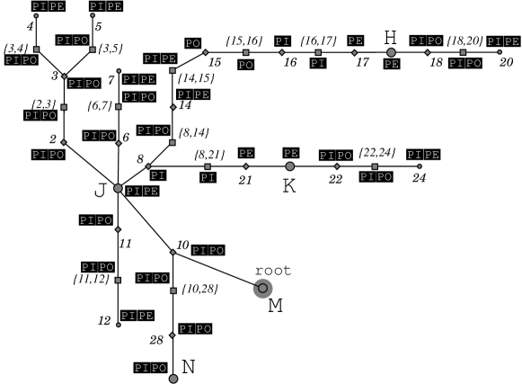
Figure 5: The $\mathcal{ABC}$-tree in Figure 4 tagged after completion of the labelling phase.

The graph shown in Figure 4 admits two robust MISs shown in Figures 7 and 7.

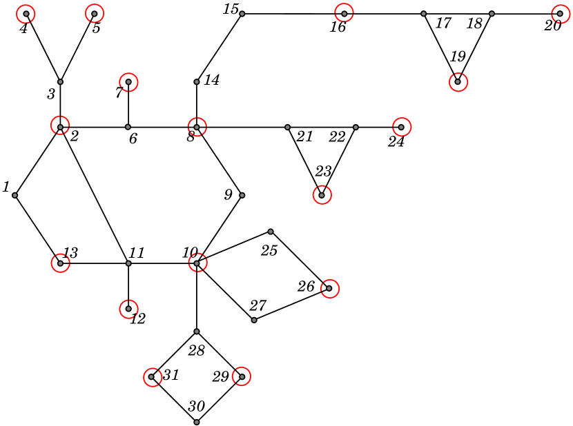
Figure 6: One possible RMIS of $G$ that includes $16$ vertices.

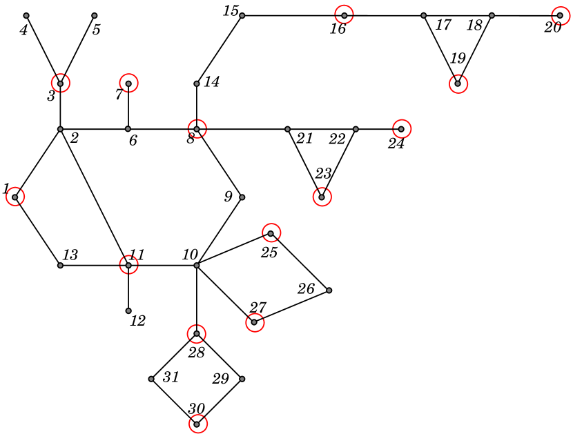
Figure 7: Another possible RMIS of $G$ that includes $14$ vertices.

References

- [1] Eleni C Akrida, Leszek Gasieniec, George B Mertzios, and Paul G Spirakis. On temporally connected graphs of small cost. In International Workshop on Approximation and Online Algorithms (WAOA), pages 84–96. Springer, 2015.
- [2] Dana Angluin, James Aspnes, Zoë Diamadi, Michael J. Fischer, and René Peralta. Computation in networks of passively mobile finite-state sensors. Distributed Computing, 18(4):235–253, 2006.
- [3] Baruch Awerbuch and Shimon Even. Efficient and reliable broadcast is achievable in an eventually connected network. In Proceedings of the third annual ACM symposium on Principles of distributed computing (PODC), pages 278–281. ACM, 1984.
- [4] Leonid Barenboim and Michael Elkin. Sublogarithmic distributed MIS algorithm for sparse graphs using nash-williams decomposition. Distributed Computing, 22(5-6):363–379, 2010.
- [5] Nicolas Braud Santoni, Swan Dubois, Mohamed Hamza Kaaouachi, and Franck Petit. The next 700 impossibility results in time-varying graphs. International Journal of Networking and Computing, 6(1):27–41, 2016.
- [6] Arnaud Casteigts and Paola Flocchini. Deterministic algorithms in dynamic networks: Problems, analysis, and algorithmic tools. In tech. report commissioned by Defense Research and Development Canada (DRDC), 2013.
- [7] Arnaud Casteigts, Paola Flocchini, Walter Quattrociocchi, and Nicola Santoro. Time-varying graphs and dynamic networks. IJPEDS, 27(5):387–408, 2012.
- [8] Swan Dubois, Mohamed-Hamza Kaaouachi, and Franck Petit. Enabling minimal dominating set in highly dynamic distributed systems. In 17th International Symposium on Stabilization, Safety, and Security of Distributed Systems (SSS), pages 51–66, 2015.
- [9] Pierre Fraigniaud, Amos Korman, and David Peleg. Local distributed decision. In Foundations of Computer Science (FOCS), 2011 IEEE 52nd Annual Symposium on, pages 708–717. IEEE, 2011.
- [10] Zoltán Füredi. The number of maximal independent sets in connected graphs. Journal of Graph Theory, 11(4):463–470, 1987.
- [11] Jerrold R Griggs, Charles M Grinstead, and David R Guichard. The number of maximal independent sets in a connected graph. Discrete Mathematics, 68(2-3):211–220, 1988.
- [12] C. Gómez-Calzado, A. Casteigts, M. Larrea, and A. Lafuente. A connectivity model for agreement in dynamic systems. In 21st Int. Conference on Parallel Processing (EUROPAR), volume 9233 of Lecture Notes in Computer Science, pages 333–345, Vienna, Austria, 2015.
- [13] Valerie King. Lower bounds on the complexity of graph properties. In Proceedings of the twentieth annual ACM symposium on Theory of computing (STOC), pages 468–476. ACM, 1988.
- [14] Fabian Kuhn, Nancy A. Lynch, and Rotem Oshman. Distributed computation in dynamic networks. In Proc. of the 42nd ACM Symposium on Theory of Computing (STOC), pages 513–522, 2010.
- [15] Christoph Lenzen and Roger Wattenhofer. MIS on trees. In Proceedings of the 30th symposium on Principles of distributed computing (PODC), pages 41–48. ACM, 2011.
- [16] Nathan Linial. Locality in distributed graph algorithms. SIAM J. Comput., 21(1):193–201, 1992.
- [17] Othon Michail, Ioannis Chatzigiannakis, and Paul G Spirakis. New models for population protocols. Synthesis Lectures on Distributed Computing Theory, 2(1):1–156, 2011.
- [18] John W Moon and Leo Moser. On cliques in graphs. Israel journal of Mathematics, 3(1):23–28, 1965.
- [19] Moni Naor and Larry J. Stockmeyer. What can be computed locally? SIAM J. Comput., 24(6):1259–1277, 1995.
- [20] Regina O’Dell and Roger Wattenhofer. Information dissemination in highly dynamic graphs. In Joint Workshop on Foundations of Mobile Computing (DIALM-POMC), pages 104–110, 2005.
- [21] Alessandro Panconesi and Aravind Srinivasan. On the complexity of distributed network decomposition. Journal of Algorithms, 20(2):356–374, 1996.
- [22] Masafumi Yamashita and Tsunehiko Kameda. Computing on anonymous networks. i. characterizing the solvable cases. IEEE Transactions on parallel and distributed systems, 7(1):69–89, 1996.