Discriminative models for multi-instance problems with tree-structure

Abstract

Modeling network traffic is gaining importance in order to counter modern threats of ever increasing sophistication. It is though surprisingly difficult and costly to construct reliable classifiers on top of telemetry data due to the variety and complexity of signals that no human can manage to interpret in full. Obtaining training data with sufficiently large and variable body of labels can thus be seen as prohibitive problem. The goal of this work is to detect infected computers by observing their HTTP(S) traffic collected from network sensors, which are typically proxy servers or network firewalls, while relying on only minimal human input in model training phase. We propose a discriminative model that makes decisions based on all computer’s traffic observed during predefined time window (5 minutes in our case). The model is trained on collected traffic samples over equally sized time window per large number of computers, where the only labels needed are human verdicts about the computer as a whole (presumed infected vs. presumed clean). As part of training the model itself recognizes discriminative patterns in traffic targeted to individual servers and constructs the final high-level classifier on top of them. We show the classifier to perform with very high precision, while the learned traffic patterns can be interpreted as Indicators of Compromise. In the following we implement the discriminative model as a neural network with special structure reflecting two stacked multi-instance problems. The main advantages of the proposed configuration include not only improved accuracy and ability to learn from gross labels, but also automatic learning of server types (together with their detectors) which are typically visited by infected computers.

1 Motivation

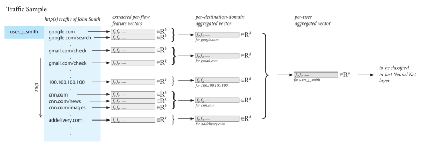
Figure 1: Sketch of the traffic of a single computer.

In network security it is increasingly more difficult to react to influx of new malicious programs like trojans, viruses and others (further called malware). Traditional defense solutions rely on identifying pre-specified patterns (called signatures) known to distinguish malware in incoming network connections, e-mails, locally stored programs, etc. But signature-matching now looses breath with the rapid increase in malware sophistication. Contemporary sophisticated malware deploys many evasion techniques such as polymorphism, encryption, obfuscation, randomization, etc, which critically decrease recall of signature-based methods. The perpendicular approach is identifying infected computers on the basis of their behavior, i.e., usually by monitoring and evaluating network activity or system calls. The advantage of the latter approach is higher recall, because it is much harder to evade behavior-based detection. E.g., computers infected by spamming malware almost inevitably display an increase in number of sent e-mails. Click-fraud, where infected computers earn money to the originator of infection by showing or accessing advertisements, is another example where the increased volume of certain traffic is a good indicator of compromise. On the other hand, behavior-based malware detection frequently suffers from higher false positive rate compared to signature based solutions.

Machine learning methods have been recently in focus due to their promise to improve false-positive-rate of behavioral malware detection[2]. However, the use of off-the-shelf machine learning methods to detect malware is typically hindered by the difficulty to obtaining accurate labels, especially if classification is to be done on the level of individual network connections (TCP flow, HTTP request, etc.)[11, 13]. Even for an experienced security analyst it is almost impossible to determine which network connections are initiated by malware and which by a benign user or application, since malware often mimics behavior of benign connections. We have observed malware connecting to google.com for seemingly benign connection checks, displaying advertisements, or sending e-mail as mentioned above. Labeling individual network connections is thus prohibitive not only due to their huge numbers but also due to ambiguity of individual connection’s classification. Automatic and large-scale training of accurate classifiers is thus very difficult.

In this work we sidestep this problem by moving the object of classification one level up, i.e., instead of classifying individual connections we classify the computer (a collection of all its traffic) as a whole. The immediate benefit is twofold. First, the labeling is much simpler, as it is sufficient to say “this computer is infected / clean” rather than “this connection has been caused by malware”. Second, a grouping of connections provides less ambiguous evidence than a single connection (see cases described above where a single access of ad server does not tell much, but multitude of such accesses does). This latter property is in fact the main motivation behind our present work.

The biggest obstacle in implementing a classifier on basis of all observed traffic is the variability in the number of network connections (hereafter called flows). This property effectively rules out majority of machine learning algorithms requiring each sample to be described by a fixed dimensional vector, because the number of observed flows supposed to characterize one computer can range from dozens to millions while the flows may vary in information content. Our problem thus belongs to the family of multi-instance learning (MIL) problems [3, 7] where one sample is commonly called a bag (in our case representing a computer) and consists of a variable number of instances (in our case one instance is one flow), each described by a fixed dimensional vector.

The solution proposed below differs from common MIL paradigm by taking a step further and representing data not as a collection of bags, but as a hierarchy of bags. We show that such approach is highly advantageous as it effectively utilizes natural hierarchy inherent to our data. Flows emitted or observed by one computer can be easily grouped according to servers they connect to (these groups are called sub-bags), so that the bag representing the particular computer becomes a collection of sub-bags. This hierarchy can be viewed as a tree with leafs representing flows (instances), inner nodes representing servers (sub-bags), and finally the root representing the computer (bag). The structure of the problem is shown in Figure 1. Note that trees representing different computers will have different number of inner nodes and leafs. The proposed classifier exploits this structure by first modeling servers (sub-bags) on basis of flows targeted to them and then modeling the computer on top of the server models. This approach can be viewed as two MIL problems stacked one on top of the other. In Section 3 we show how the hierarchical MIL problem can be mapped into neural-network architecture, enabling direct use of standard back-propagation as well as many recent developments in the field of deep learning. Once trained, the architecture can be used for classification but it can also be dismantled to identify types of traffic significant for distinguishing benign from infected computer, i.e., it allows to extract learned indicators of compromise (IoCs). Finally, using approach similar to URCA [17], it is possible to identify particular connections which made the neural network decide that the computer is infected; hence effectively providing an explanation of the learned IoC.

Section 4 demonstrates the proposed approach on large scale real problem of detecting infected computers from proxy logs. It is shown that the network can learn to identify infected computers in protected network, as well as provide sound explanation of its verdicts to the consumer. Neurons in lower layer are shown to have learned weak indicators of compromise typical for malware.

The proposed neural architecture is shown to have multiple advantageous properties. Its hierarchal MIL nature dramatically reduces the cost of label acquisition. By using labels on high-level entities such as computers or other network devices the creation of training data is much simpler. The ability to dismantle the encoded structure is no less important as it provides definition of learned indicators of compromise. Finally, it allows human understandable explanation of classifier verdict as security incident, which simplifies the job of the network administrator.

This paper is organized as follows. The next section formulates the problem of multiple instance learning and reviews important work we build upon. The proposed approach is presented in Section 3 Experimental evaluation is provided in Section 4.

2 Related work

In the following we review the evolution of paradigms leading to the solution proposed in next chapter.

2.1 Multi instance learning problem

The pioneering work [6] coined multiple-instance or multi-instance learning as a problem, where each sample $b$ (to be denoted bag in the following) consists of a set of instances $x$, i.e., $b=\{x_{i}\in\mathcal{X}|i\in\{1,\ldots|b|\}\}.$ Each instance $x$ can be attributed a label $y_{x}\in\{-1,+1\},$ but these instance-level labels are not assumed to be known even in the training set. The sample $b$ was deemed positive, if at least one of its instances had a positive label, i.e., label of a sample $b$ is $y=\max_{x\in b}y_{x}.$ For this scenario the prevalent approach is the so-called instance-space paradigm, i.e., to train a classifier on the level of individual instances $f:\mathcal{X}\mapsto\{-1,+1\}$ and then infer the label of the bag $b$ as $\max_{x\in b}f(x).$

2.1.1 Embedded-Space Paradigm

Later works (see reviews [3, 7]) have introduced different assumptions on relationships between the labels on the instance level and labels of bags or even dropped the notion of instance-level labels and considered only labels on the level of bags, i.e., it is assumed that each bag $b$ has a corresponding label $y\in\mathcal{Y},$ which for simplicity we will assume to be binary, i.e., $\mathcal{{Y}}=\{-1,+1\}$ in the following. The common approach of the latter type is either to follow a bag-space paradigm and define a measure of distance (or kernel) between bags or to follow an embedded-space paradigm and define a transformation of the bag to a fixed-size vector.

Since the solution presented in Section 3 belongs to the embedded-space paradigm, we describe this class of methods in necessary detail and adopt the formalism of [16], which is for our solution essential. The formalism of [16] is intended for a general formulation of MIL problems, where labels are assumed only on the level of bags without any labels on the level of instances. Each bag $b$ consists of a set of instances, which are viewed as a realization of some probability distribution $p_{b}$ defined over the instance space $\mathcal{X}$. To allow more flexibility between bags even within the same class, the formalism assumes that probability distributions $p_{b}$ of different bags are different, which is captured as $p_{b}$ being realization of a probability $P(p_{b},y$), where $y\in\mathcal{Y}$ is the bag label.

During the learning process each concrete bag $b$ is thus viewed as a realization of unknown probability distribution $p_{b}$ that can be inferred only from groups of instances $\{x\in b|x\sim p_{b}\}$ observed in data. The goal is to learn a discrimination function $f:\mathcal{B}\mapsto\mathcal{Y},$ where $\mathcal{B}$ is the set of all possible realizations of all distributions $p\in\mathcal{P}^{\mathcal{X}}$, i.e., $\mathcal{B}=\left\{x_{i}|p\in\mathcal{P}^{\mathcal{X}},x_{i}\sim p,i\in\{1,\ldots l\},l\in\mathbb{N}\right\}$. Note that this definition also includes that used in [6].

Methods from embedded space-paradigm [3, 7] first represent each bag $b$ as a fixed-dimensional vector and then use any machine learning algorithm with samples of fixed dimension. Therefore the most important component in which most methods differ is the embedding. Embedding of bag $b$ can be generally written as

$$\left(\phi_{1}(b),\phi_{2}(b),\ldots,\phi_{m}(b)\right)\in\mathbb{R}^{m}.$$ (1)

with individual projection $\phi_{i}:\mathcal{B}\mapsto\mathbb{R}$ being

$$\phi_{i}=g\left(\left\{k(x,\theta_{i})\right\}_{x\in b}\right),$$ (2)

where $k:\mathcal{X}\times\Theta\mapsto\mathbb{R}_{0}^{+}$ is a suitably chosen distance function parametrized by parameters $\theta$ (also called dictionary items) and $g:\cup_{n=1}^{\infty}\mathbb{R}^{k}\mapsto\mathbb{R}$ is the pooling function (e.g. minimum, mean or maximum). Most methods differ in the choice of aggregation function $g,$ distance function $k,$ and finally in selection of dictionary items $\theta\in\Theta$.

2.2 Simultaneous Optimization of Embedding and Classifier

Figure 2: Neural network optimizing the embedding in embedding-space paradigm.

The important novelty introduced in [16] is that embedding functions $\{\phi_{i}\}_{i=1}^{m}$ are optimized simultaneously with the classifier that uses them, as opposed to the prior art where the two optimization problems are treated indepedently. Simultaneous optimization is achieved by using the formalism of neural network, where one (or more) lower layers followed by a pooling layer implement the embedding function $\phi,$ and subsequent layers implement the classifier that is thus built on top of bag representation in form of a feature vector of fixed length. The model is sketched in Figure 2 with a single output neuron implementing a linear classifier once the embedding to a fixed-length feature representation is realized. The neural network formalism enables to optimize individual components of the embedding function as follows.

• Lower layers (denoted in Figure 2 as $\{k_{i}\}_{i=1}^{m})$ before pooling identifies parts of the instance-space $\mathcal{X},$ where the probability distributions generating instances in positive and negative bags differs the most with respect to the chosen pooling operator.

• The pooling function $g$ can be either fixed to mean or maximum, or other pooling function such that it is possible to calculate gradient with respect to its inputs. The pooling function itself can have parameters that can be optimized during learning, as was shown e.g. in [9], where the pooling function has form $\sqrt[q]{\frac{1}{|b|}\sum_{i\in b}|x_{i}|^{q}}$ with the parameter $q$ being optimized.

• Layers after the pooling (denoted in Figure 2 as $f(\cdot)$) optimize the classifier that already uses representation of the bag as vector of fixed dimension.

The above model is very general and allows automatic optimization of all parameters by means of back-propagation, though the user still needs to select the number of layers, number of neurons in each layer, their transfer function, and possibly also the pooling function.

3 The proposed solution

In the light of the previous paragraph, the problem of identifying infected computers can be viewed as two MIL problems, one stacked on top of the other, where the traffic of a computer $b$ is generated by a two-level generative model.

3.1 Generative Model

Let us denote $\mathcal{S}$ the set of all servers accessible by any computer. Let $\mathcal{S}_{c}\subseteq\mathcal{S}$ denote the selection of all servers accessed from computer $c$ in given time frame. The communication of computer $c$ with each server $s\in\mathcal{S}_{c}$ consists of a group of flows $x\in\mathcal{X}$ that are viewed as instances forming a first-level bag $b_{s}$. Bag of flows $b_{s}$ is thus viewed as a realization of some probability distribution $p_{b_{s}}\in\mathcal{P}^{\mathcal{X}}$ .

We imagine that every server $s$ is associated with a type $t(s),$ which influences the probability distribution of the flows $p_{b_{s}}$. Accordingly, each first-level bag $b_{s}$ is realized according to $p_{b_{s}}$ which itself is a realization of a probability distribution $P(p_{b_{s}},t(s)).$ This captures the real-world phenomenon of user’s interaction with some server (e.g., e-mail server) being different from that of a different user communicating with the same server, as well as the fact that different types of servers impose different communication patterns.

In view of the above we can now consider computer $c$ to be the second-level bag consisting of a group of first-level bags $b_{s}$. Similarly to the above we assume $c$to be a realization of probability distribution $p_{c}\in\mathcal{P}^{\mathcal{B}}$ where $\mathcal{B}$ is the set of all possible realizations of all distributions $p\in\mathcal{P}^{\mathcal{X}}$. Probability distribution $p_{c}$ is expected to be different for each computer, particularly we assume this to be true between infected and clean computers labeled by $y\in\{-1,+1\}$. Probability distribution $p_{c}$ is thus viewed as realization of a probability distribution $P(p_{c},y)$. This captures the real-world observation that infected computers exhibit differences in communication patterns to servers, both in selection of servers and inside individual connections to the same server.

input : $y\in\{-1,+1\}$ label marking computer as clear or infected

output : Set of flows $\mathcal{F}$ of one computer

1. sample a distribution $p_{c}$ of servers from $P(p_{c},y)$;

2. sample a set of servers $\mathcal{S}_{c}$ from $p_{c}$;

3. $\mathcal{F}=\textrm{\O}$;

foreach $s\in\mathcal{S}_{c}$ do %iterate over selected

       4. sample distribution $p_{b_{s}}$ of flows from $P(p_{b_{s}},t(s))$;

       5. sample flows $x$ from $p_{b_{s}}$;

       6. add sampled flows to all flows, $\mathcal{F}=\mathcal{F}\cup x$;

      

end foreach

 

Algorithm 1 Generative model of the flows of one computer.

The model imposes a generative process as illustrated in Algorithm 1.

The proposed multi-level generative model opens up possibilities to model patterns on the level of individual connections to server as well as on the level of multiple servers’ usage. In the following we discuss the implementation and show the practical advantages on large-scale experiments.

3.2 Discriminative model

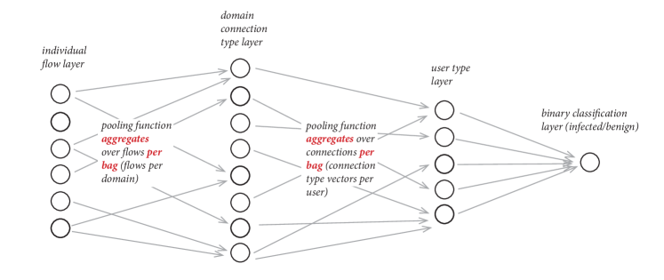
Figure 3: Hierarchical MIL

The rationale behind the discriminative model closely follows the above generative model by breaking the problem into two parts: classifying the computer on basis of types of contacted servers and classifying type of the server on basis of flows exchanged between the server and the client.

Let’s assume that each contacted server is described by a feature vector of fixed dimension, which can be as simple as one-hot encoding of its type $t(s).$ Then the problem of classifying the computer becomes a MIL problem with bag being the computer and instances being servers. The problem is of course that type servers $t(s)$ are generally unknown and we cannot imagine to manually create a mapping between server IP or domain name and server type. To make the problem even more difficult, the same server can be used differently by different computers, and therefore it can be of different type for each of them. One can indeed learn a classifier that would predict the server type from flows between the computer and the server, which again corresponds to MIL classifier with the bag being the server and instances being the flows, but the problem of labeled samples for training the classifier is non-trivial and it is unlikely that we will have known all types of servers. Moreover, since we are learning a discriminative model, we are interested in types of server occurring with different probabilities in clean and infected computers.

To side step this problem we propose to stack MIL classifier on the level of computers on top of the MIL classifier on the level of servers. Since both MIL classifiers are realized by a neural network described in the previous chapter, we obtain one (bigger) neural network with all parameters optimizable using standard back-propagation and importantly using labels only on the level of bag (computer). This effectively removes the need to know types of servers $t(s)$ or learn classifier for them, because the network learns that automatically from the labels on the level of computers. The caveat is that the network learns only types of servers occurring with different probabilities in clean and infected computers.

The idea in its simplest incarnation is outlined in Figure 3. The distinctive feature is the presence of two pooling layers reflecting two MIL problems dividing the network into three parts. The first part part up to the first pooling included implements embedding of sub-bags into a finite-dimensional vector (modeling servers on basis of flows). After the first pooling each sub-bag (server) is represented by one finite-dimensional vector. Similarly the second part starting between the first pooling up to the second pooling included embeds sub-bags into a finite dimensional vector characterizing each bag (computer). Finally, the third part starting after to second pooling implements the final classifier.

The right choice of the pooling function is not straightforward with many aspects to be taken into the consideration.

• $\mathrm{Mean}$ function should be theoretically better [12], since it is more general. The advantage of $\mathrm{mean}$ pooling function has been experimental demonstrated in [16].

• If malware performs few very distinct types of connections (e.g. connection checks) even though they would go to well known servers, $\max$ functions can identify them whereas $\mathrm{mean}$ function might suppress them among the clutter caused by many connections of legitimate applications. This problem has been recently studied in [4] in context of natural images.

• The number of contacted servers and flows to servers varies between computers and $\mathrm{max}$ pooling is more stable then $\mathrm{mean}.$

• The training with $\max$ pooling is approximately six times faster, since the back-propagation is non-zero only for one element entering the pooling operation (one flow per server and neuron, one server per computer and neuron).

3.3 Extracting indicators of compromise

The presented model is based on the assumption that there exist types of servers contacted with different probability by infected and clean computers, though one generally does not know much about them. If these types would not exists, then the probability distributions $p_{c}$ of infected and clean computers would be the same and it would be impossible to create a reliable detector for them. But if the neural network has learned to recognize them, items of vector representation of servers (output of network’s first part (from the input to the first pooling included in Figure 3) has to have different probability distributions for clean and infected computers.

Since the above line of reasoning can be extended to the output of the layer just before the first pooling function, output of each neuron of this layer can be viewed as an indicators of compromise, since it has to contribute to the identification of infected computers. From a close inspection of flows on which these neurons provide the highest output a skilled network analyst can figure out, what kind of traffic it is (a concrete examples are shown in Section 4.2). Admittedly, these learned IOCs would deliver poor performance if used alone. But in the neural network they are used together with IOCs from different servers, which provides a context leading to good accuracy. Also, once a network administrator annotates these neurons, this annotation can be used to provide more detailed information about the decisions.

3.4 Explaining the decision

Neural networks have a reputation being a black-box in the sense that they do not provide any details about the decision. In the intrusion detection this behavior is undesirable, since the investigation of the security has to start from the very beginning. Therefore giving the investigator explanation why the classifier view the computer as infected is of great help.

The explanation method relies on the assumption that flows caused by the infection are additive, i.e. the malware does not block user’s flows but adds its own. This means that if the computer was deemed infected, by removing right flows (instances) the network should flip its decision. Although finding the smallest number of such flows is likely an NP complete problem, a greedy approximation inspired by [17] performs surprisingly well.

The greedy approximation finds in each iteration set of flows going to same server (subbag), which causes the biggest decrease of classifier’s output when removed from computer’s traffic (in our implementation positive means infected). Iterations are stopped when classifier’s output becomes negative (clean). The set of all removed subbags is returned as the explanation in the form: “This computer was found infected because it has communicated with these domains”. Examples of flows to these domains might be obviously supplied.

3.5 Computational complexity

The computational complexity is important not only for the training, but also for the deployment as the amount of network traffic that needs to be processed can be high. For example Cisco’s Cognitive Threat Analytics [5] processes $10^{10}$ HTTP logs per day. The hierarchical aggregation inside the network decreases substantially the computational complexity, since after the first pooling, the network have one vector for server instead to for one vector per flow yielding to six fold decrease of the data to be processed. Similarly, after the second pooling the computer is described just by a single vector instead of set of vectors, which against decreases the complexity. Compare this to the prior art on solving MIL with Neural Network [18], where the pooling is done after the last linear layer just before the output, which means that all layers of the network process all flows. The effect on the computational complexity is tremendous. Whereas our approach takes approximately five seconds per 100 iterations of the training, the prior art of [18] takes 1100 seconds, which is 220 times slower.

4 Experimental evaluation

Albeit the proposed solution si general and can be utilized to any type of network traffic, it has been evaluated in the context of detecting infected computers from logs of web proxies due to availability of large data to us. Besides, proxy logs are nicer for human’s investigation than for example netflow data. The proxy logs were collected by Cisco’s Cognitive Threat Analytics [5] from 500 large networks during eight days. The days were picked randomly from the period from November 2015 till February 2016 with the testing day being 7th March 2016. Since the total number of infected computers in the dataset from seven training days was small, we have added data of infected computers from additional 25 days from the period of training data.

Since the data were collected in five-minute long time windows, one bag consists of all web request of one computer during that window. Computers were identified either by source IP address or by the user name provided in proxy logs. Subbags contained requests with the same host part in the HTTP request.

Computers (bags) were labeled using Cisco’s Cognitive Threat Analytics [5] such that if one computer had at least one request known to be caused by malware, the computer was considered to be infected in that five-minute window. If the same computer in different time window did not have any malware flows, the bag from that time window was considered as clean.

The training set contained data from from approximately 20 million unique computers out of which 172 013 were infected and approximately 850 000 000 flows, out of which 50 000 000 belonged to infected computers. The testing set contained data of approximately 3 000 000 computers out of which 3 000 were infected and approximately 120 000 000 flows with 500 000 flows belonging to the infecting computers.

We are certain that labeling we have used in this experiment is far from being perfect. While there will be relatively small number number of infected computers labeled as clean, there will be quite a lot of computers labeled as clean while being infected. Despite these issues, we consider this labeling as a ground truth, because the aim of the experiments is to demonstrate that the proposed solution can learn from high-level labels and identify weak indicators of compromise.

The experiments were implemented in author’s own library, since popular libraries for neural networks are not designed for MIL problems. They do not allow to have samples (bags and sub-bags) of different sizes (number of instances) which makes the encoding of the hierarchical structure impossible. Therefore evaluated architectures used simple building blocks: rectified linear units [8, 12], mean and maximum pooling functions, and ADAM optimization algorithm [10]. Unless said otherwise, ADAM was used with default parameters with the gradient estimated in each iteration from $1000$ legitimate and $1000$ infected computers (bags) sampled randomly. This size of the minibatch is higher then is used in most art about deep learning, however we have find it beneficial most probably because the signal to be detected is weaker. Contrary to most state of the art, we have used weighted Hinge loss function $\max\left\{0,1-y\cdot w^{y}\cdot f(x)\right\}$ with $w^{\mathrm{+}}$ being the cost of (false negative) missed detection and $w^{-}$ being the cost of false positive (false alarms). The rationale behind Hinge loss is that it produces zero gradients if sample (bag) is classified correctly with sufficient margin. This means that gradient with respect to all network parameters is zero, therefore the back-propagation does not need to be performed, which leads to considerable speed-up. The learning was stopped after ADAM has performed $3\cdot 10^{5}$ iterations.

The performance was measured using precision-recall curve (PR curve) [14] popular in document classification and information retrieval due to its better properties for highly imbalanced problems, into which intrusion detection belongs (in the testing data there is approximately one infected computer per one thousand clean ones).

4.1 Network architecture

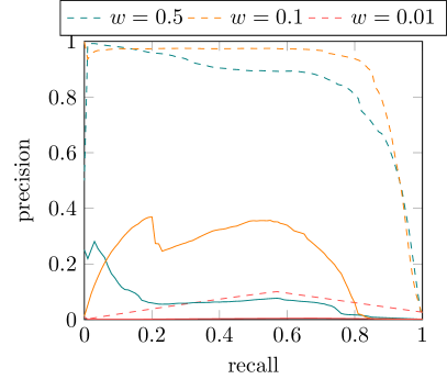
(a) relu-max-relu-max-lin

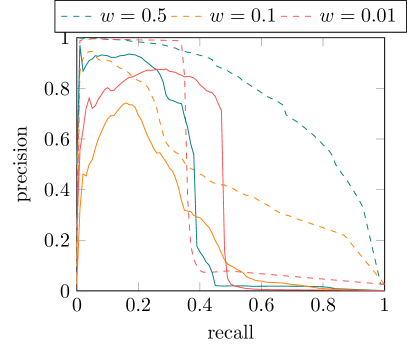
(b) relu-mean-relu-mean-lin

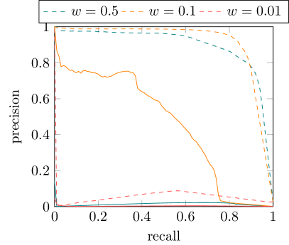
(c) relu-max-relu-max-relu-lin

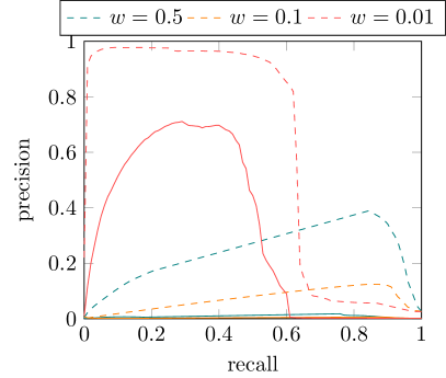
(d) relu-mean-relu-mean-relu

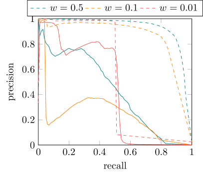
(e) relu-max-relu-relu-max-relu-lin

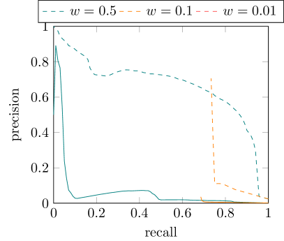
(f) relu-mean-relu-relu-mean-relu-lin

Figure 4: Precision recall curves of six neural network architectures utilizing simple $36$ features. Dashed lines shows the curves estimated on the training set and solid lines shows the curves estimated from the training set. Networks with PR curves in the left column used $\mathrm{max}$ pooling function, whereas those with PR curves in the right column used $\mathrm{mean}$ pooling function. Captions $w=0.5,$ $w=0.1,$ and $w=0.01$ corresponds to different costs in weighted hinge loss with cost on false positives (false alarms) being $w^{-}=1-w$ while that on the false negatives (missed detections) being $w^{+}=w.$

All evaluated neural networks used simple feature vectors (instances) with $36$ cheap to compute statistics, such as length of the url, query and path parts, frequency of vowels and consonants, HTTP status, port of the client and the server, etc, but not a single feature was extracted from the hostname. Evaluated neural networks followed the architecture in Figure 3 with layer of 40 ReLu neurons before the first pooling, but then differing in: using either $\mathrm{mean}$ or $\mathrm{max}$ pooling functions; having either one layer with 40 ReLu neurons or two layers each with 20 ReLu neurons between first and second pooling; and finally having additional layer of 20 ReLu neurons after the second pooling and final linear output neuron.

Precision-recall curves of all six evaluated neural networks each trained with three different costs of errors on false positive (0.9,0.99,0.999) and false negative (0.1,0.01,0.001) are shown in Figure 4. On basis of these experiments, we have made following conclusions.

• Simpler networks with $\mathrm{max}$ pooling function tends to overfit, as the error on the training set of all three evaluated architectures is very good (dashed line) but the error on the testing set is considerably worse. We believe this to be caused by the network to act more like a complicated signature detector by learning a specific patterns in flows prevalent in the infected computers in the training set, but missing in infected computers in testing set. This hypothesis is supported by (i) the fact that when we have been creating ground truth, we have labeled computer as infected if it had at least one connection known to be caused by malware and (ii) testing data being one month older then training ones.

• Simple networks with $\mathrm{mean}$ pooling with costs of error $w^{\mathrm{+}}=0.01$ and $w^{-}=0.99$ are amongst the best ones. Their discrepancy between training and testing error is much lower then in the case of $\mathrm{max}$ pooling, except the most complicated architecture 4f. We believe this to be caused by the network learning how infected computers behave (contacting too many advertisement servers) rather than patterns specific for some type of the malware (like those with $\mathrm{max}$ pooling). This conclusion is supported by the fact that $\mathrm{max}$ pooling function can be approximated from the $\mathrm{mean}$ if layers preceding the aggregation are sufficiently complicated [15].

Interesting feature is sharp drop in precision of certain architectures, which we attribute to the fact that some infections cannot be detected with used simple 34 features.

4.2 Indicators of compromise

Since one of the main features of the proposed architecture is an ability to learn indicators of compromise IOCs, below it is shown to what types of traffic neurons in the layer just before the first pooling are sensitive. The sensitivity was estimated from infected computers in the testing set for the simplest architectures (top row in Figure 4) with $\mathrm{mean}$ and $\mathrm{max}$ pooling functions.

We have not observed much difference between IOCs learned by network with $\mathrm{mean}$ and $\mathrm{max}$ pooling functions. Learned IOCs included:

• tunneling through url (example shown in appendix due to its length);

• sinkholed domains such as hxxp://malware.vastglows.com, hxxp://malware.9f6qmf0hs.ru/a.htm?u=396923, hxxp://malware.ywaauuackqmskc.org/.

• domains with repetitive characters such as hxxp://wwwwwwwwwwwwvwwwwwwwwwwwwwwwwwwvwwwwwwwwwwwwwwwwwwwwwwwwwwwwvww.com/favicon.ico or hxxp://ibuyitttttttttttttttttttttttttttttttttttibuyit.com/xxx.zip;

• https traffic to raw domains such as hxxps://209.126.109.113/;

• subdomain generated by an algorithm on a hosting domain, for example d2ebu295n9axq5.webhst.com, d2e24t2jgcnor2.webhostoid.com, or dvywjyamdd5wo.webhosteo.com;

• Download of infected seven-zip: d.7-zip.org/a/7z938.exe.

4.3 Example of explanation

NN
output	url
4.84	hxxp://www.inkstuds.org/?feed=podcast
2.07	hxxp://feeds.podtrac.com/YxRFN5Smhddj
0.21	hxxps://www.youtube-nocookie.com/
0.18	hxxps://upload.wikimedia.org/

Table 1: Example output of the explanation of an incident.

Table 1 shows an explanation of the simplest evaluated neural network with maximum pooling functions. The explanation consists of a list of domains with examples of requests to them as they have been identified by the greedy algorithm described in Section 3.4. The column captioned “NN output” shows, how the output of the neural net decreases as flows to individual domains are iteratively removed.

At the time of writing this paper, the last three domains were all involved in the communication with some malware samples according to VirusTotal [1]. Searching further on a web we have found this article stating that www.inkstuds.org have been hacked and used to serve malware.

5 Conclusion

We have introduced stacked Multiple Instance Learning architecture, where data is viewed not as a collection of bags but as a hierarchy of bags. This extension of MIL paradigm is shown to bring many advantages particularly for our targeted application of intrusion detection. The hierarchical model is straightforward to implement, requiring just a slight modification of a standard neural network architecture. This enables to exploit vast neural network knowledgebase including deep learning paradigms.

The proposed architecture posses key advantages especially important in network security. First, it requires labels (clean / infected) only on the high level of computers instead of on single flows, which dramatically saves time of human analyst constructing the ground truth and also makes it more precise (it might be sometimes nearly impossible to determine, if the flow is related to infection or not). Second, the learned mapping of traffic patterns to neurons can be extracted to obtain human understandable Indicators of Compromise. Third, it is possible to identify flows, which have cased the computer to be classified as infected, which decreases time needed to investigate the security incident.

The advantages of the proposed architecture were demonstrated in the context of detecting infected computers from their network traffic collected on the proxy server. It has been shown that the neural network can detect infected computers, learn indicators of compromise in lower layers from high-level labels, and provide sound explanation of the classification.

Appendix A Types of learned IOCs

• tunneling through urls

hxxp://call.api.bidmatic.com/event/click/e54ae5b5435b118ca6539752037be726e1d6ccbd297e8ce191ad1304c2d813e9b0739b9699e4f69b370663ef3476aa3a4e6b15fd4dbe392849711a223e5635d088bad54f4aeee18fcf830b72c2c6588f5a3faf4db8cf39b5aa5b1ee77bb5cd4254f666a6295ec4c47c9eea5cdd612bcdd9541430f58e27d2d5f36700526f94106ad7bfae9409dcc7d6897be9e015724fcd66e5564ab56f4e1be62456237f7567d667a95f3b24ea2ef127b75e5cc353104579b047f09c5e01eab79a57935692e9be881eec56c4030a01b4ffa7bcdc72430ffe1a8b091182851016c299a8b343f1cc015f6cc9b36e109334b04bfef24b15acf0b0cb4bad9bd9523dbffe0e0171e6f180ce475c3fdd701a33c6a144f135e8d651f54ca92a4fa572938bc248471991542aba5e5f380d5b00c7931384d0a726b1a27db83ceb1178e7355e1451a9e8f8ac91c7306aff1f23be85849b51dfa52f8bb52f1be5cdf5497d739a8760c7c7178a811d7e2555e864bbd5b32840e65862aac63c266a0c6dd72468ae975982db1135322d604d43b62c1259f22677d15ee2dbd86fdfefe84807c66999d87cdaaa92edf007466f73ee2bc14a6d5ee708649c5f7caf814e4497826308a508d4ff94eb91d55ca2e44e02e2ff8740ac7f1c16135319c38eba9fd50e397edf8a98afbc2e1bd18e82208c6109f253370ca95d035aac4edf6e8ef51ab891b85e5b2bf6e8ce3480bc4c69ac505ca31397f7133716ba5d8652d716999c4ecac7b787f663ac6fb0b32a6b6fe10eb740397e893cb58b49bc2ed18b10944d5e149c5935e367f43d94d074ab8b2f732d34e194be43f7f940

hxxp://s.crbfmcjs.info/dealdo/shoppingjs4?b=Chy9mZaMDhnSpxvUzgvMAw5LzczKyxrHpsu3qIuYmMGXCYuYmIuZqsu1qIuYmIu1q24LmJaLmJaLmJaLmJaLmJaLmJaLmJaLmJaLmJaLmJaLmJaLmJaLmJaLmJaLmJaLmJaLmJaLmJaLmJaLmJaLmJaLmJaLmJaLmJaLmJaLmJaLnunUjtiWjtiWjtiWjtiWjtiWjtiWjtiWjtiWjtiWjtiWjtiWjtiWjtiWjtiWjtiWjtiWjtiWjtiWjtiWjtiWjtiWjtiWjtiWjtiWjtiWjtiWjtvdBIuYmcuYmcuYmcuYmcuYmcuYmfrLEMeLmJbSysuYmg1HDgvTyxrPy2eLmJbZzw0UmI1JBgfZysuYmgeLmJa3lweLmJaLmJaLmJaLmJiLnuqLmKmLmJj0AxrSzsuYmIuZqsuYmLrLEMeLmJbSysuYmg1HDgvTyxrPy2eLmJbZzw0UmI1JBgfZysuYmgeLmJa3lweLmJaLn0mLmJbZB3jPBMjVCM9KAsuYmcu3qYuYmde0lJa1lJiWmtaLmJiLmKmLmJjKB21HAw4LmJiLm0eLmJj3D3CUzgLKywn0AwmUCM8LmJiLmKmLmJj1CMWLmJiLm0eLmJjODhrWjtnbjtjgjtjgD3D3lMrPzgfJDgLJlNjVjtjgBwf0zxjPywXLlwrPzgfJDgLJzsuYrJeYnZeZm190zxPHlwXHlw1HDgvTyxrPy2eTC2vTltiTy2XHC2eTys03lweLmJiLmKmLmJjLBMmLmJiLm0eLmJjvveyTocuYmIuYqYuYmNDUyw1LjtiYjtnbjtiYjtiYjtjdjtiYAxndB21yjtiYjtnbjtiYt0SLm0fKzwyWjtiYjtjdjtiYzYuYmIuZqsu3qIu3rcuYqYuYmMrWu2vZC2LVBKLKjtiYjtnbjtiYmtq2ndaXodKYmdu0odG0mtyLmJiLmKmLmJjezwfSugX5jtiYjtnbjtiYBNjJEwnMExvZjtiYjtjdjtiYzg1UjtiYjtnbjtiYzgLKywn0AwmUCM8LmJiLmKmLmJjMAxjZDfrPBwuLmJiLm0eLmJjMywXZzsuYmIu3rczJBhy9mtq2mtu2ntq4odmYoczXBt0WjMnIptG0oszWyxj0BMvYpwnYyMzTyYzOCMq9mtuWmgiZytnInMfJmJDLmJHJnJjLmwuYyMeWodDHytGMAhjKC3jJpsz2zwHPy2XLpszJAgfUBMvSpwnYyMzTy2nYzhjFmJaWmZe2mZe4ndmZmdaWmdaWjNnZzxq9nczHChb0purLywXiDxqMAxr5Cgu9AszLEhq9x18MDha9BNvSBcz2CJ0MBhrPBwu9mtq2ndaXodKYmdG0oszKB209y3jIzM1JANmUAw5MBYzZzwXMps4Mzg9TCMvMzxjYzxi9Ahr0CcuYntnbjti1mKyLmJuYrND3DY5KAwrHy3rPyY5YBYuYntjgBwf0zxjPywXLlwrPzgfJDgLJzsuYntjgDgv6ys1TyxrLBwf0AwnHlwnSyxnHlweTn2eMCgXPBMS9jMHSAw5RpszWCM9KDwn0CZ0MAw5ZDgDYCd0MAwfNpwnSAwvUDdeWmc4UjMnVB2TPzxntDgf0Dxm9y29VA2LLrw5HyMXLza==

References

- [1] Virus total. https://www.virustotal.com, 2016.
- [2] Tansu Alpcan and Tamer Başar. Network security: A decision and game-theoretic approach. Cambridge University Press, 2010.
- [3] Jaume Amores. Multiple instance classification: Review, taxonomy and comparative study. Artificial Intelligence, 201:81–105, 2013.
- [4] Y-Lan Boureau, Jean Ponce, and Yann LeCun. A theoretical analysis of feature pooling in visual recognition. In Proceedings of the 27th international conference on machine learning (ICML-10), pages 111–118, 2010.
- [5] Cisco Systems Inc. Cisco Cognitive Threat Analytics. https://cognitive.cisco.com.
- [6] Thomas G Dietterich, Richard H Lathrop, and Tomás Lozano-Pérez. Solving the multiple instance problem with axis-parallel rectangles. Artificial intelligence, 89(1):31–71, 1997.
- [7] James Foulds and Eibe Frank. A review of multi-instance learning assumptions. The Knowledge Engineering Review, 25(01):1–25, 2010.
- [8] Xavier Glorot, Antoine Bordes, and Yoshua Bengio. Deep sparse rectifier neural networks. In Aistats, volume 15, page 275, 2011.
- [9] Caglar Gulcehre, Kyunghyun Cho, Razvan Pascanu, and Yoshua Bengio. Learned-norm pooling for deep feedforward and recurrent neural networks. In Machine Learning and Knowledge Discovery in Databases, pages 530–546. Springer, 2014.
- [10] Diederik Kingma and Jimmy Ba. Adam: A method for stochastic optimization. arXiv preprint arXiv:1412.6980, 2014.
- [11] Matthew V. Mahoney and Philip K. Chan. Learning nonstationary models of normal network traffic for detecting novel attacks. In Proceedings of the Eighth ACM SIGKDD International Conference on Knowledge Discovery and Data Mining, KDD ’02, pages 376–385, New York, NY, USA, 2002. ACM.
- [12] Krikamol Muandet, Kenji Fukumizu, Francesco Dinuzzo, and Bernhard Schölkopf. Learning from distributions via support measure machines. In Advances in neural information processing systems, pages 10–18, 2012.
- [13] T. T. T. Nguyen and G. Armitage. A survey of techniques for internet traffic classification using machine learning. IEEE Communications Surveys Tutorials, 10(4):56–76, Fourth 2008.
- [14] James W. Perry, Allen Kent, and Madeline M. Berry. Machine literature searching x. machine language; factors underlying its design and development. American Documentation, 6(4):242–254, 1955.
- [15] T. Pevný and I. Nikolaev. Optimizing pooling function for pooled steganalysis. In Information Forensics and Security (WIFS), 2015 IEEE International Workshop on, pages 1–6, Nov 2015.
- [16] Tomáš Pevný and Petr Somol. Using neural network formalism to solve multiple-instance problems. In submission to ECML 2016.
- [17] F. Silveira and C. Diot. Urca: Pulling out anomalies by their root causes. In INFOCOM, 2010 Proceedings IEEE, pages 1–9, March 2010.
- [18] Zhi-hua Zhou and Min-ling Zhang. Neural networks for multi-instance learning. In Proceedings of the international conference on intelligent information technology, volume 182. Citeseer, 2002.