Constrained clustering via diagrams:
A unified theory and its applications to electoral district design

Abstract

The paper develops a general framework for constrained clustering which is based on the close connection of geometric clustering and diagrams. Various new structural and algorithmic results are proved (and known results generalized and unified) which show that the approach is computationally efficient and flexible enough to pursue various conflicting demands.

The strength of the model is also demonstrated practically on real-world instances of the electoral district design problem where municipalities of a state have to be grouped into districts of nearly equal population while obeying certain politically motivated requirements.

1 Introduction

Constrained Clustering

General clustering has long been known as a fundamental part of combinatorial optimization and data analytics. For many applications (like electoral district design) it is, however, essential to observe additional constraints, particularly on the cluster sizes. Accordingly, the focus of the present paper is on constrained clustering where a given weighted point set $X$ in some space $\mathcal{X}$ has to be partitioned into a given number $k$ of clusters of (approximately) predefined weight.

As has been observed for several applications, good clusterings are closely related to various generalizations of Voronoi diagrams; see e.g. [15], [30], [20] for recent work that is most closely related to the present paper. Besides electoral district design, such applications include grain-reconstruction in material sciences ([1]), farmland consolidation ([10], [15], [11]), facility and service districting ([55], [59], [45], [46], [40], [29], [3]), and robot network design ([21], [19]).

We will present a general unified theory which is based on the relation of constrained geometric clustering and diagrams. In Sections 2 and 3, we analyze the model and prove various favorable properties.

Using several types of diagrams in different spaces, we obtain partitions that are optimized with respect to different criteria: In Euclidean space, we obtain clusters that are particularly well consolidated. Using locally ellipsoidal norms, we can to a certain extent preserve originally existing structures. In a discrete metric space derived from a graph that encodes an intrinsic neighboring relation, we obtain assignments that are guaranteed to be connected. In the theoretical part the various different issues will be visualized with the help of a running example.

Electoral District Design

Our prime example will be that of electoral district design which has been approached from various directions over the last half century (see [51], [38], and [56] for surveys, [32] for the example of Germany, and [36], [37] for general accounts on partitions). Municipalities of a state have to be grouped to form electoral districts. The districts are required to be of nearly equal population and of “reasonable” shape. Hence a crucial nature of the electoral district design problem is that there are several partly conflicting optimization criteria such as the grade of population balance, consolidation, or a desire for some continuity in the development of districts over time. Therefore we will show how our unified approach allows the decision maker to compare several models with different optimization foci.

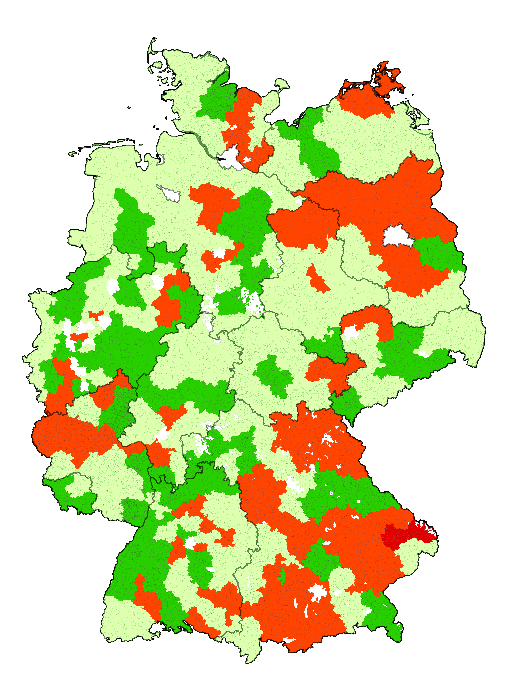
(a) Deviations of the 2013 election districts in Germany

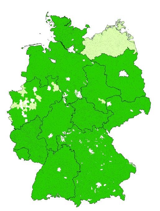
(b) Deviations resulting from our methodology.

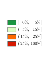
(c) Colors depict the deviation from the federal average district size.

Figure 1: Absolute deviations from the average population size per district.

Section 4 will show the effect of our method for the federal elections in Germany. The German law ([25]) requires that any deviation of district sizes of more than 15% from the federal average is to be avoided. As a preview, Figure 1 contrasts the occurring deviations from the 2013 election with the deviations resulting from one of our approaches. The federal average absolute deviation drops significantly from 9.5% for the 2013 election to a value ranging from 2.1% to 2.7% depending on the approach. For most states, these deviations are close to optimal since the average district sizes of the states i.e., the ratios of their numbers of districts and eligible voters differ from the federal average already about as much. See Section 4 for detailed results and the Appendix for further statistics. Furthermore, an online supplement depicts the results of all approaches for the full data set, see http://www-m9.ma.tum.de/material/districting/.

Constrained Clustering via Generalized Voronoi Diagrams

In accordance with [22], the generalized Voronoi diagram for given functions $f_{i}:\mathcal{X}\rightarrow\mathbb{R}$, $i=1,\ldots,k$, is obtained by assigning each point $x\in\mathcal{X}$ to a subset $C_{i}$ of $\mathcal{X}$ whose value $f_{i}(x)$ is minimal. We are interested in clusterings of $X$ that are induced by such diagrams (cf. Section 2.2).

Of course, in order to obtain suitable diagrams, the choice of the functions $f_{i}$ is crucial. For parameters $(\mathcal{D},h,\mathcal{S},\mathcal{M})$ we define the $k$-tuple of functions $\mathcal{F}(\mathcal{D},h,\mathcal{S},\mathcal{M}):=\left(f_{1},\ldots,f_{k}\right)$ via

$$f_{i}(x):=h(d_{i}(s_{i},x))+\mu_{i}.$$

Here, $\mathcal{D}:=\left(d_{1},\ldots,d_{k}\right)$ is a $k$-tuple of metrics (or more general distance measures) on $\mathcal{X}$, $h:\mathbb{R}_{\geq 0}\rightarrow\mathbb{R}_{\geq 0}$ is monotonically increasing, $\mathcal{S}:=\left(s_{1},\ldots,s_{k}\right)\in\mathcal{X}^{k}$ is a $k$-tuple of points in $\mathcal{X}$, and $\mathcal{M}:=(\mu_{1},\ldots,\mu_{k})\in\mathbb{R}^{k}$ is a vector of reals. If the metrics $d_{i}$ are not all identical, we call the resulting diagram anisotropic.

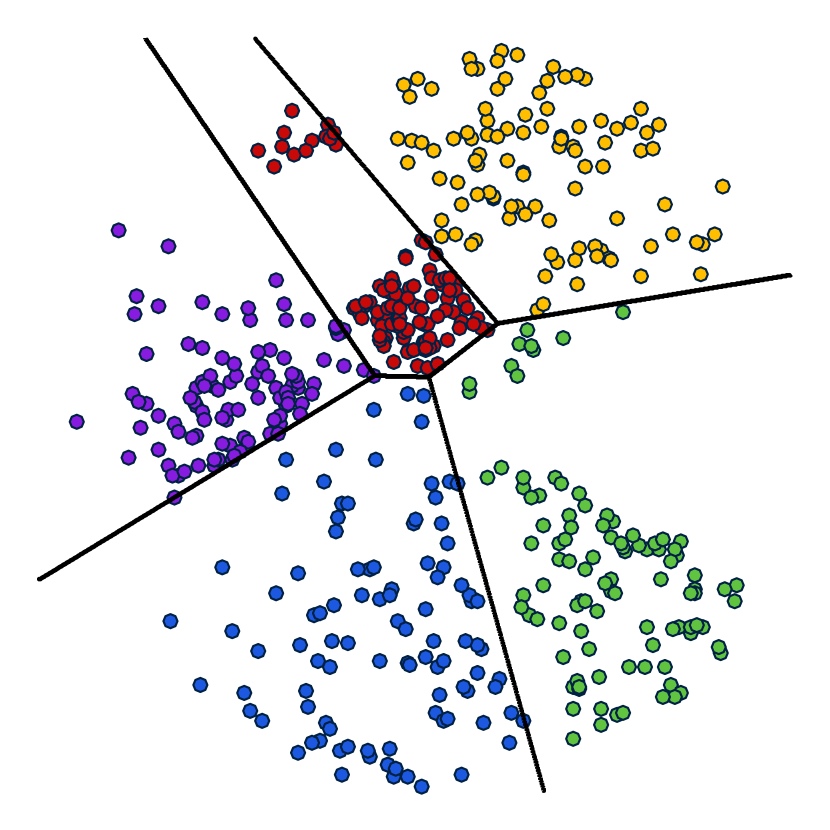
(a) Diagram in Euclidean space.

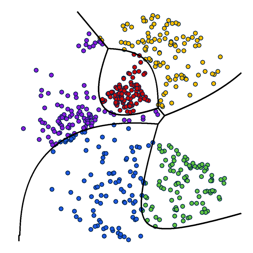
(b) Anisotropic diagram with local ellipsoidal norms.

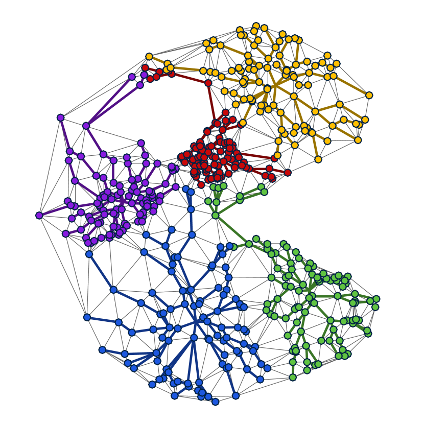
(c) Diagram in discrete space.

Figure 2: Exemplary clusterings and related diagrams.

We consider an exemplary selection of types of generalized Voronoi diagrams (see also [4], [22], [48], [50]). For each of the considered types, Figure 2 depicts an exemplary diagram together with its induced clustering.

In the Euclidean space, the choice

$$f_{i}(x):=\left\lVert x-s_{i}\right\rVert_{2}^{2}+\mu_{i}$$

yields power diagrams; see [5], [8]. For the particular case of centroidal diagrams, in which the sites coincide with the resulting centers of gravity of the clusters, the inherent variance is minimized. This can be achieved by optimization over $\mathcal{S}$ (cf. [15], [14], [9], [28]).

The setting

$$f_{i}(x):=\left\lVert x-s_{i}\right\rVert_{2}+\mu_{i}$$

yields additively weighted Voronoi diagrams.

Allowing for each cluster an individual ellipsoidal norm yields anisotropic Voronoi and power diagrams, respectively. Appropriate choices of norms facilitate the integration of further information such as the shape of pre-existing clusters in our application.

We also consider the discrete case $\mathcal{X}=X$. Here, we are given a connected graph $G:=(X,E,\delta)$ with a function $\delta:E\rightarrow\mathbb{R}_{>0}$ assigning a positive distance to each edge. With $d_{G}(x,y)$ defined as the length of the shortest $x$-$y$-path in $G$ w. r. t. $\delta$, this induces a metric on $\mathcal{X}$. The choice of

$$f_{i}(x):=d_{G}(s_{i},x)+\mu_{i}$$

then leads to shortest-path diagrams. Such diagrams guarantee the connectivity of all clusters in the underlying graph. This allows to represent intrinsic relations of data points that cannot be easily captured otherwise.

As we will see, the parameters $\mathcal{D}$ and $h$ mainly determine the characteristics of the resulting diagrams. The points $s_{i}$ then serve as reference points – called sites – for the clusters.

It is shown that for any choice of $\mathcal{D}$, $h$ and $\mathcal{S}$ there exists a choice of the additive parameter tuple $\mathcal{M}$, such that the induced clusters are of prescribed weight as well as optimally consolidated (cf. Corollary 2). Thus, we distinguish between the structural parameters $\mathcal{D},h$ and $\mathcal{S}$ and the feasibility parameter $\mathcal{M}$. Our approach does not automatically yield integral assignments in general but may require subsequent rounding. However, the number of fractionally assigned points and thus the deviation of cluster weights can be reasonably controlled (see 5).

Typically, $\mathcal{D}$ and $h$ are defined by the specific application as it determines the requirements on the clusters. One can still optimize over the remaining structural parameter $\mathcal{S}$ with respect to different criteria, e. g., optimal total variances or margins. For any choice of structural parameters, the feasibility parameter $\mathcal{M}$ is then readily provided as the dual variables of a simple linear program.

As we will point out in more detail our framework extends various previously pursued approaches. We feel that a unified and self-contained exposition serves the reader better than a treatment that relies heavily on pointers to the scattered literature. Hence we include occasionally new concise proofs of known results whenever this adds to the readability of the paper. Of course, we try to always give the appropriate references.

Organization of the Paper

Section 2 yields the general definitions and methodology for our approach. Section 3 provides a short study of typical generalized Voronoi diagrams and shows their relevance for constrained clustering. Section 4 then presents our results for the electoral district design problem for the example of Germany in all detail, while Section 5 concludes with some final remarks.

2 Definitions and Methodology

We begin by describing our approach to constrained geometric clustering in a general context. Due to the specific application we focus on the discrete case of partitioning a given finite weighted set; some results for the continuous case will however also be mentioned.

First, Section 2.1 defines the terminology for constrained clusterings. We construct clusterings that are induced by a suitable dissection of the underlying space. For this purpose, Section 2.2 formally defines generalized types of Voronoi diagrams and shows how they relate to clusterings. Section 2.3 then yields the main theoretical results that establish a correspondence of clusterings with prescribed capacities and generalized Voronoi diagrams.

2.1 Constrained Clustering

Let $k,m\in\mathbb{N}$ and $\mathcal{X}$ be an arbitrary space. We consider a set

$$X:=\{x_{1},\ldots,x_{m}\}\subset\mathcal{X}$$

with corresponding weights

$$\Omega:=(\omega_{1},\ldots,\omega_{m})\in\mathbb{R}_{>0}^{m}.$$

Furthermore, let

$$\mathcal{K}:=(\kappa_{1},\ldots,\kappa_{k})\in\mathbb{R}_{>0}^{k}$$

such that $\sum_{i=1}^{k}\kappa_{i}=\sum_{j=1}^{m}\omega_{j}$.

The vector $\mathcal{K}$ contains the desired cluster ”sizes”. Hence, we want to find a partition of $X$ such that for each cluster $C_{i}$ its total weight meets the prescribed capacity $\kappa_{i}$.

For $k=2$, integer weights, and $\kappa_{1}=\kappa_{2}$ the associated decision problem coincides with the well-known Partition problem and is therefore already ${\mathcal{NP}}$-hard.

We consider also a relaxed version of the problem by allowing fractional assignments

$$\mathcal{C}:=\left(\xi_{i,j}\right)_{\begin{subarray}{c}i=1,\ldots,k\\ j=1,\ldots,m\end{subarray}}\in[0,1]^{k\times m}$$

such that $\sum_{i=1}^{k}\xi_{i,j}=1$ for each $j$. $\mathcal{C}$ is called a (fractional) clustering of $X$ and $\xi_{i,j}$ is the fraction of unit $j$ assigned to cluster $i$. We further set $C_{i}:=(\xi_{i,1},\ldots,\xi_{i,m})$, call it cluster $i$ and let

$$\operatorname{supp}(C_{i}):=\{x_{j}\in X:\xi_{i,j}>0\}$$

denote its support, i. e., the set of those elements in $X$ that are assigned to $i$ with some positive fraction. If $\mathcal{C}\in\{0,1\}^{k\times m}$, we call the clustering integer.

The weight of a cluster is given by

$$\omega(C_{i}):=\sum_{j=1}^{m}\xi_{i,j}\omega_{j}.$$

A clustering $\mathcal{C}$ is strongly balanced, if

$$\omega(C_{i})=\kappa_{i}$$

for each $i$. If lower and upper bounds $\kappa^{-}_{i},\kappa^{+}_{i}\in\mathbb{R}_{\geq 0}$ for the cluster weights are given and

$$\kappa^{-}_{i}\leq\sum_{j=1}^{m}\omega_{j}\xi_{i,j}\leq\kappa^{+}_{i}$$

holds for every $i$, $\mathcal{C}$ is called weakly balanced. A case of special interest for our application is that of $\kappa^{-}_{i}=(1-\epsilon)\kappa_{i}$ and $\kappa^{+}_{i}=(1+\epsilon)\kappa_{i}$ for all $i$ for some given $\epsilon>0$. Then, i.e., if

$$(1-\epsilon)\kappa_{i}\leq\omega(C_{i})\leq(1+\epsilon)\kappa_{i}$$

for each $i$ we call $\mathcal{C}$ $\epsilon$-balanced, or, whenever the choice of $\epsilon$ is clear simply balanced.

By $\operatorname{BC}$ and $\operatorname{BC}^{\epsilon}$ we denote the set of all strongly balanced and $\epsilon$-balanced fractional clusterings, respectively. Note that the condition $\sum_{i=1}^{k}\kappa_{i}=\sum_{j=1}^{m}\omega_{j}$ guarantees that $\operatorname{BC}\neq\emptyset$. Similarly, let $\operatorname{BC}_{I}$ and $\operatorname{BC}_{I}^{\hskip 1.0pt\epsilon}$ denote the set of all strongly balanced and $\epsilon$-balanced integer clusterings, respectively. Of course, $\operatorname{BC}_{I}\subset\operatorname{BC}\subset\operatorname{BC}^{\epsilon}$ and $\operatorname{BC}_{I}\subset\operatorname{BC}_{I}^{\hskip 1.0pt\epsilon}\subset\operatorname{BC}^{\epsilon}$.

2.2 Clusterings induced by Generalized Voronoi Diagrams

Let a $k$-tuple $\mathcal{F}:=\left(f_{1},\ldots,f_{k}\right)$ of functions $f_{i}:\mathcal{X}\rightarrow\mathbb{R}$ for $i=1,\ldots,k$ be given. For each cluster, the corresponding $f_{i}$ is supposed to act as a distance measure. While a classical Voronoi diagram in Euclidean space assigns each point to a reference point which is closest, this concept can be generalized by assigning a point to each region for which the corresponding value of $f_{i}$ is minimal. Formally, we set

$$P_{i}:=\{x\in\mathcal{X}:f_{i}(x)\leq f_{l}(x)~{}\forall l\in\{1,\ldots,k\}\}$$

and call $P_{i}$ the $i$-th (generalized) Voronoi region (or cell). Then $\mathcal{P}:=(P_{1},\ldots,P_{k})$ is the generalized Voronoi diagram (w. r. t. $\mathcal{F}$).

Note that, in general, $\mathcal{P}$ does not constitute a partition of $\mathcal{X}$. We will, of course, in the application focus on choices of the functions $f_{i}$ that guarantee that the cells $P_{i}$ do not have interior points in common; see Lemma 6.

A generalized Voronoi diagram $\mathcal{P}$ is said to be feasible for a clustering $\mathcal{C}$ if

$$\operatorname{supp}(C_{i})\subset P_{i}$$

for all $i$. Typically, we do not want a Voronoi region to contain elements “by chance”, i. e., points that are not (at least fractionally) assigned to their corresponding cluster. Hence, we say $P$ supports $\mathcal{C}$, if

$$\operatorname{supp}(C_{i})=P_{i}\cap X$$

for all $i$.

2.3 Correspondence of Constrained Clusterings and Generalized Voronoi Diagrams

As described in the introduction, we are interested in finding a clustering $\mathcal{C}\in\operatorname{BC}$ that is supported by a generalized Voronoi diagram $\mathcal{P}$ w. r. t. functions $f_{i}(x):=h(d_{i}(s_{i},x))+\mu_{i}$. A natural question is for which choices of $(\mathcal{D},h,\mathcal{S},\mathcal{M})$ such a clustering exists.

By definition, a diagram $\mathcal{P}$ is feasible for $\mathcal{C}\in\operatorname{BC}$ if and only if

$$\xi_{i,j}\cdot\left(h(d_{i}(s_{i},x_{j}))+\mu_{i}-\min_{l=1,\ldots,k}(h(d_{l}(s_{l},x_{j}))+\mu_{l})\right)=0$$ (1)

holds for every $i=1,\ldots,k$ and $j=1,\ldots,m$.

We will now recover (1) as a complementary slackness condition in linear programming. For this purpose, first note that in general, i. e., for any $\mathcal{C}\in\operatorname{BC}$ and $(\mathcal{D},h,\mathcal{S},\mathcal{M})$, we have

$$\sum_{i=1}^{k}\sum_{j=1}^{m}\xi_{i,j}\cdot\omega_{j}\cdot\left(h(d_{i}(s_{i},x_{j}))+\mu_{i}-\min_{l=1,\ldots,k}(h(d_{l}(s_{l},x_{j}))+\mu_{l})\right)\geq 0,$$ (2)

as all weights $\omega_{j}$ are positive and each factor in the sum above is non-negative. Using $\sum_{j=1}^{m}\omega_{j}\xi_{i,j}=\kappa_{i}$ for each $i$ and $\sum_{i=1}^{k}\xi_{i,j}=1$ for each $j$, Inequality (2) is equivalent to

$$\sum_{i=1}^{k}\sum_{j=1}^{m}\xi_{i,j}\cdot\omega_{j}\cdot h(d_{i}(s_{i},x_{j}))\geq\sum_{j=1}^{m}\omega_{j}\min_{l=1,\ldots,k}(h(d_{l}(s_{l},x_{j}))+\mu_{l})-\sum_{i=1}^{k}\kappa_{i}\mu_{i}.$$ (3)

Note that (1) holds for every $i$ and $j$ if and only if (2), and hence (3), holds with equality.

Now, observe that the left-hand side of (3) does not depend on $\mathcal{M}$ while the right-hand side does not depend on $\mathcal{C}$. For any choice of $(\mathcal{D},h,\mathcal{S})$ equality in (3) can therefore only hold if $\mathcal{C}$ minimizes the left-hand side while $\mathcal{M}$ maximizes the right-hand side. Thus, in particular, $\mathcal{C}\in\operatorname{BC}$ must be a minimizer of the linear program

$$\begin{array}[]{p{20pt}>{\displaystyle}r@{}>{\displaystyle}l@{\hspace{5pt}}o@{\hspace{5pt}}r@{\hspace{15pt}}>{\displaystyle}l}\lx@intercol\displaystyle\min\limits_{\mathcal{C}\in\mathbb{R}^{k\times m}}\sum_{i=1}^{k}\sum_{j=1}^{m}\xi_{i,j}\cdot\omega_{j}\cdot h(d_{i}(s_{i},x_{j}))~{}~{}\text{ s.t. }\hfil\lx@intercol\\ &\sum_{i=1}^{k}\xi_{i,j}&\hfil\hskip 5.0&={}\hfil\hskip 5.0&1\hskip 15.0&(i=1,\ldots,k)\\ &\sum_{j=1}^{m}\xi_{i,j}&\omega_{j}\hfil\hskip 5.0&={}\hfil\hskip 5.0&\kappa_{i}\hskip 15.0&(j=1,\ldots,m)\\ &\xi_{i,j}&\hfil\hskip 5.0&\geq{}\hfil\hskip 5.0&0\hskip 15.0&(i=1,\ldots,k;j=1,\ldots,m).\end{array}$$ (P)

By introducing auxiliary variables $\mathcal{E}:=(\eta_{1},\ldots,\eta_{m})$, maximization of the right-hand side of (3) can be formulated as linear program, as well:

$$\begin{array}[]{p{7pt}>{\displaystyle}r@{\hspace{2pt}}o@{\hspace{2pt}}>{\displaystyle}r@{\hspace{5pt}}>{\displaystyle}l}\lx@intercol\displaystyle\max_{{\begin{subarray}{c}\mathcal{M}\in\mathbb{R}^{k},\\ \mathcal{E}\in\mathbb{R}^{m}\end{subarray}}}\hskip 1.99997pt\sum_{j=1}^{m}\omega_{j}\eta_{j}-\sum_{i=1}^{k}\kappa_{i}\mu_{i}~{}~{}\text{ s.t. }\hfil\lx@intercol\\ &\eta_{j}\hskip 2.0&\leq{}\hfil\hskip 2.0&h(d_{i}(s_{i},x_{j}))+\mu_{i}\hskip 5.0&(i=1,\ldots,k;j=1,\ldots,m)\end{array}$$ (D)

Now, observe that (D) is the dual program to (P). Thus, $\mathcal{P}$ is feasible for $\mathcal{C}$ if and only if $\mathcal{C}$ and $(\mathcal{M},\mathcal{E})$ are primal-dual optimizers. In particular, as

$$\eta_{j}=\min_{i=1,\ldots,k}(h(d_{l}(s_{i},x_{j}))+\mu_{i})$$

holds for every optimal solution of (D), Equation 1 states exactly the complementary slackness conditions. Furthermore, if the complementarity is strict, i. e., exactly one factor is strictly positive in any equation of type (1), this is equivalent to $\mathcal{P}$ supporting $\mathcal{C}$.

We summarize these observations in the following theorem.

Theorem 1.

Let $\mathcal{C}\in\operatorname{BC}$, $\mathcal{D}$ be a $k$-tuple of metrics on $\mathcal{X}$, $\mathcal{S}\in\mathcal{X}^{k}$, $h:\mathbb{R}_{\geq 0}\rightarrow\mathbb{R}$, $\mathcal{M}\in\mathbb{R}^{k}$, and let $\mathcal{P}$ be the generalized Voronoi diagram w. r. t. $\mathcal{F}(\mathcal{D},h,\mathcal{S},\mathcal{M})$. Further, set $\eta_{j}:=\min_{i=1,\ldots,k}(h(d_{i}(s_{i},x_{j}))+\mu_{i})$ for $j=1,\ldots,m$, and $\mathcal{E}:=(\eta_{1},\ldots,\eta_{m})$,

Then $(\mathcal{M},\mathcal{E})$ is feasible for (D) and the following equivalencies hold:

$\mathcal{P}$ is feasible for $\mathcal{C}$	$\Leftrightarrow$	$\mathcal{C}$ and $(\mathcal{M},\mathcal{E})$ satisfy the complementary slackness condition for (P) and (D)
$\mathcal{P}$ supports $\mathcal{C}$	$\Leftrightarrow$	$\mathcal{C}$ and $(\mathcal{M},\mathcal{E})$ satisfy the strict complementary slackness condition for (P) and (D)

1 establishes a one-to-one-correspondence of (fractional) strongly balanced clusterings that are supported by a generalized Voronoi diagram and those faces of the polytope $\operatorname{BC}$ which are optimal w. r. t. a corresponding objective function.

Observe that the deduction of 1 did not use any further assumptions on the functions $f_{i}$ besides the additive component $\mathcal{M}$. Thus, we obtain the following corollary.

Corollary 2.

Let $\hat{f}_{i}:\mathcal{X}\rightarrow\mathbb{R}$, $i=1,\ldots,k$. Then $\mathcal{C}^{\ast}\in\operatorname{BC}$ is an optimizer of $\min_{\mathcal{C}\in\operatorname{BC}}\sum_{i=1}^{k}\sum_{j=1}^{m}\xi_{i,j}\cdot\omega_{j}\cdot\hat{f}_{i}(x_{j})$ if and only if there exists $\mathcal{M}:=(\mu_{1},\ldots,\mu_{k})\in\mathbb{R}^{k}$ such that the generalized Voronoi diagram w. r. t. $f_{i}:=\hat{f}_{i}+\mu_{i}$ is feasible for $\mathcal{C}^{\ast}$.

For functions $\hat{f}_{i}(x):=h(d_{i}(s_{i},x))$, this has already been shown by linear programming duality in [15] for a discrete set $X$, $h=(\cdot)^{2}$, and the Euclidean metric. In a continuous setting, i. e., for $X=\mathbb{R}^{n}$ and balancing constraints defined w. r. t. a probability distribution on $\mathbb{R}^{n}$, this has been proven in [5] and extended to more general function tuples $\mathcal{F}$ in [30]. Here, the particular case $h={\operatorname{id}}$ is contained in [3]. In [21], this result was deduced for the Euclidean case and an arbitrary function $h$ by carefully considering the optimality conditions of an alternative optimization problem and deducing optimality (but not establishing the linear programming duality). Furthermore, in [19] and [20] the general continuous case was proved by discretization also involving linear programming duality.

Using the second part of 1, we can now characterize supporting diagrams.

Corollary 3.

Let $\hat{f}_{i}:\mathcal{X}\rightarrow\mathbb{R}$, $i=1,\ldots,k$. Then $\mathcal{C}^{\ast}\in\operatorname{BC}$ lies in the relative interior of the optimal face of $\min_{\mathcal{C}\in\operatorname{BC}}\sum_{i=1}^{k}\sum_{j=1}^{m}\xi_{i,j}\cdot\omega_{j}\cdot\hat{f}_{i}(x_{j})$ if and only if there exists $\mathcal{M}:=(\mu_{1},\ldots,\mu_{k})\in\mathbb{R}^{k}$ such that the generalized Voronoi diagram w. r. t. $f_{i}:=\hat{f}_{i}+\mu_{i}$ supports $\mathcal{C}^{\ast}$.

Thus, for non-unique optima the supporting property of the diagrams may still be established but comes with the price of more fractionally assigned elements (cf. Section 3.3).

Another fact that roots in a basic result about extremal points of transportation polytopes has been noted in their respective context by several authors (e. g., [55], [44], [59], [34], [31], [39], [15]): An optimal basic solution of (P) yields partitions with a limited number of fractionally assigned points.

Our proof of the following Lemma 4 relies on the bipartite assignment graph $H(\mathcal{C})$ that is associated with a given clustering $\mathcal{C}\in\operatorname{BC}$. It is defined by

$$H(\mathcal{C}):=(\{1,\ldots,k\}\cup X,E)$$

with

$$E:=\{\{i,x_{j}\}:\xi_{i,j}>0\}.$$

By [41, Thm. 4] $H(\mathcal{C})$ is acyclic if and only if $\mathcal{C}$ is extremal, i. e., a vertex of the feasible region of (P).

Lemma 4.

Let $\hat{f}_{i}:\mathcal{X}\rightarrow\mathbb{R}$, $i=1,\ldots,k$. Then there exists $\mathcal{M}:=(\mu_{1},\ldots,\mu_{k})\in\mathbb{R}^{k}$ and a clustering $\mathcal{C}\in\operatorname{BC}$ with at most $(k-1)$ fractionally assigned points and at most $2(k-1)$ fractional components $\xi_{i,j}$ such that the generalized Voronoi diagram w. r. t. $f_{i}:=\hat{f}_{i}+\mu_{i}$ is feasible for $\mathcal{C}$.

Proof.

Let $\mathcal{C}$ be an extremal solution of (P) and $H(\mathcal{C})=(\{1,\ldots,k\}\cup X,E)$ be the corresponding assignment graph. As $H(\mathcal{C})$ is acyclic it follows that $|E|\leq k+m-1$. Further, from the definition of $\operatorname{BC}$ it follows that $\deg(x_{j})\geq 1$ for every $j=1,\ldots,m$. Moreover, for any fractionally assigned element $x_{j}\in X$ it follows that $\deg(x_{j})\geq 2$. As $H(\mathcal{C})$ is bipartite, we also have that $|E|=\sum_{j=1}^{m}\deg(x_{j})$. In conclusion, this yields

$$k+m-1 \geq|E|=\sum_{j=1}^{m}\deg(x_{j})\geq m+\frac{1}{2}\left|\{\{i,x_{j}\}:0<\xi_{i,j}<1\}\right|$$

$$\geq m+\left|\{x_{j}\in X:x_{j}\text{ is fractionally assigned}\}\right|,$$

which implies the assertion. ∎

Note that for the special case of $\omega_{j}=1$ for all $j$ every extremal solution of the transportation problem (P) is integral, i. e., $\operatorname{BC}=\operatorname{BC}_{I}$ (cf. [41, Corollary 1]). In general, however, this is not the case.

Anyway, by solving the linear program (P) and applying suitable rounding, we obtain an integer clustering that satisfies an a-priori (and for many applications very reasonable) error bound. More precisely, [54] showed that minimizing the maximum error after rounding can be done in polynomial time using a dynamic programming approach, while minimizing the sum of absolute or squared errors is ${\mathcal{NP}}$-hard. In [34] it was furthermore shown that minimizing the number of fractional assignments while obeying a pre-defined error tolerance is ${\mathcal{NP}}$-hard.

The following theorem provides an upper bound for $\epsilon$ that guarantees the existence of an $\epsilon$-balanced integer clustering.

Theorem 5.

Let $\hat{f}_{i}:\mathcal{X}\rightarrow\mathbb{R}$, $i=1,\ldots,k$ and $\epsilon\geq\max_{1\leq j\leq m,1\leq i\leq k}\frac{\omega_{j}}{\kappa_{i}}$. Then there exists $\mathcal{C}\in\operatorname{BC}_{I}^{\hskip 1.0pt\epsilon}$ together with $\mathcal{M}:=(\mu_{1},\ldots,\mu_{k})\in\mathbb{R}^{k}$, such that the generalized Voronoi diagram w. r. t. $f_{i}:=\hat{f}_{i}+\mu_{i}$ is feasible for $\mathcal{C}$.

For rational input, i. e., $\Omega\in\mathbb{Q}^{m}_{>0},\mathcal{K}\in\mathbb{Q}^{k}_{>0}$, $\hat{f}_{i}(x_{j})\in\mathbb{Q}$, $i=1,\ldots,k$ and $j=1,\ldots,m$, $\mathcal{C}$ and $\mathcal{M}$ can be determined in polynomial time.

Proof.

By Corollary 2 a solution $\tilde{\mathcal{C}}\in\operatorname{BC}$ of (P) with a corresponding dual solution $(\mu_{1},\ldots,\mu_{k})\in\mathbb{R}^{k}$ yields a generalized Voronoi diagram w. r. t. $f_{i}:=\hat{f}_{i}+\mu_{i}$ that is feasible for $\tilde{\mathcal{C}}$. We may furthermore choose $\tilde{\mathcal{C}}$ to be extremal. We can also assume that the assignment graph $H(\tilde{\mathcal{C}})$ is a tree (otherwise we consider its connected components). We may further root this tree in the node $1$ (that corresponds to cluster $C_{1}$) and w.l.o.g. assume that the other clusters are labelled according to their distance from the root, i. e., for $1\leq i<l\leq k$ it holds that the length of a shortest $1$-$i$-path is at most the length of a shortest $1$-$l$-path in $H(\mathcal{C})$.

For each $i=1,\ldots,k$ we denote the index sets of units that are either non-integrally or integrally assigned to cluster $C_{i}$ by

$$\begin{array}[]{ccc}F(i):=\{j:0<\tilde{\xi}_{i,j}<1\}&\text{ and }&I(i):=\{j:\tilde{\xi}_{i,j}=1\},\end{array}$$

respectively. Now, we construct an integer clustering $\mathcal{C}^{\ast}\in\{0,1\}^{k\times m}$ in which all integral assignments are preserved, i. e., $\xi_{i,j}^{\ast}:=\tilde{\xi}_{i,j}$ for $\tilde{\xi}_{i,j}\in\{0,1\}$. The remaining components will be determined successively for each cluster.

Let us begin with $C_{1}^{\ast}$. We round up fractional assignments $\xi_{i,j},j\in F(1)$, successively as long as this is allowed by the upper bound $\kappa_{1}$. More precisely, let

$$j^{\ast}:=\max\{j\in F(1):\sum\limits_{\begin{subarray}{c}r\in F(1):\\ r\leq j\end{subarray}}\omega_{r}\leq\kappa_{1}-\sum\limits_{r\in I(1)}\omega_{r}\}$$

if the set on the right-hand side is non-empty, otherwise set $j^{\ast}:=0$. With

$$\xi^{\ast}_{1,j}:=\begin{cases}1,&\text{if }j\leq j^{\ast}\\ 0,&\text{otherwise.}\end{cases}$$

for every $j\in F(1)$ it then follows that $|\sum_{j=1}^{m}\xi^{\ast}_{{1},j}\omega_{j}-\kappa_{1}|<\max_{j=1,\ldots,m}\omega_{j}$.

Now let $i_{0}\geq 2$ and assume that we have determined $C^{\ast}_{i}$ appropriately for every $i<i_{0}$. Let $x_{j_{0}}\in X$ be the predecessor of the node $i_{0}$ in the rooted tree $H(\tilde{\mathcal{C}})$. By assumption, the assignment $\xi_{i,j_{0}}^{\ast}$ of unit $x_{j_{0}}$ to cluster $C_{i}$ has already been determined for every $i<i_{0}$. We then set

$$\xi_{i_{0},j_{0}}^{\ast}:=\begin{cases}1,&\text{if }\xi_{i,j_{0}}^{\ast}=0\text{ for all }i<i_{0}\\ 0,&\text{otherwise.}\end{cases}$$ (4)

In analogy to the first step, we define

$$j^{\ast\ast}:=\max\{j\in F(i_{0})\setminus\{j_{0}\}:\sum\limits_{\begin{subarray}{c}r\in F(i_{0}):\\ r\leq j\end{subarray}}\omega_{r}\leq\kappa_{i_{0}}-\sum\limits_{r\in I(i_{0})}\omega_{r}-\xi_{i_{0},j_{0}}^{\ast}\omega_{j_{0}}\}$$

if the set on the right-hand side is non-empty, $j^{\ast\ast}:=0$ otherwise, and set

$$\xi^{\ast}_{i_{0},j}:=\begin{cases}1,&\text{if }j\leq j^{\ast\ast}\\ 0,&\text{otherwise}\end{cases}$$

for every $j\in F(i_{0})\setminus\{j_{0}\}$ .

Every point that is fractionally assigned in $\tilde{\mathcal{C}}$ is assigned either to its predecessor in $H(\tilde{\mathcal{C}})$ or to exactly one successor by (4). Thus, it holds that $\mathcal{C}^{\ast}\in\operatorname{BC}_{I}^{\hskip 1.0pt\epsilon}$. As $\operatorname{supp}(C_{i}^{\ast})\subset\operatorname{supp}(\tilde{C}_{i})$, the already obtained generalized Voronoi diagram remains feasible for $\mathcal{C}^{\ast}$.

Hence, under the additional rationality assumptions, we can solve the linear program (P) and perform the successive rounding in polynomial time. ∎

Note that the bound of 5 is asymptotically worst-case optimal (e. g., for $m=1$, $\omega_{1}=k$, $\kappa_{i}=1$ for all $i$ and letting $k\rightarrow\infty$).

As in [15], we may also consider weakly balanced clusterings where lower and upper bounds $\kappa^{-}_{i},\kappa^{+}_{i}\in\mathbb{R}_{\geq 0}$ for the cluster weights are provided. Of course, a minimizer $\mathcal{C}^{\ast}$ over the polytope of such weakly balanced clusterings is a minimizer of (P) when setting $\kappa_{i}:=\omega(C_{i}^{\ast})$ for every $i$. Hence, optimal weakly balanced clusterings still yield supporting generalized Voronoi diagrams. Unfortunately, the converse is not true in general; see [15] for an example.

Naturally, we prefer generalized Voronoi diagrams that support a clustering over diagrams that are only feasible, as they exclude the possibility of points lying in a diagram’s region only “by coincidence”. At the same time, we prefer clusterings with only few fractional assignments as provided by 5. As a consequence of Corollary 3, this coincides whenever the optimum of (P) is unique. In case of $\mathcal{X}=\mathbb{R}^{n}$, this can be guaranteed by an appropriate choice of the structural parameters $\mathcal{D},h,\mathcal{S}$. We first show that under mild assumptions the generalized Voronoi-cells behave properly.

Lemma 6.

Let $\mathcal{X}=\mathbb{R}^{n}$, $\mathcal{D}:=\left(d_{1},\ldots,d_{k}\right)$ be a family of metrics induced by strictly convex norms, $h:\mathbb{R}\rightarrow\mathbb{R}$ injective, $\mathcal{S}:=(s_{1},\ldots,s_{k})\in(\mathbb{R}^{n})^{k}$ such that $s_{i}\neq s_{l}$ for $i\neq l$, and $\mathcal{M}\in\mathbb{R}^{k}$.

Then for the generalized Voronoi diagram $\mathcal{P}$ w. r. t. $\mathcal{F}(\mathcal{D},h,\mathcal{S},\mathcal{M})$ we have $\operatorname{int}(P_{i})\cap\operatorname{int}(P_{l})=\emptyset$ whenever $i\neq l$.

Proof.

Let $B_{1},B_{2}\subset\mathbb{R}^{n}$ be the unit balls of the norms that induce $d_{1}$ and $d_{2}$, respectively. Furthermore, denote by $\left\lVert\cdot\right\rVert_{B_{i}}$, $i=1,2$, the corresponding norms, i. e., $d_{i}(x,0)=\left\lVert x\right\rVert_{B_{i}}=\min\{\rho\geq 0:x\in\rho B_{i}\}$ for every $x\in\mathbb{R}^{n}$, $i=1,2$.

Suppose that there exists $x_{0}\in\mathbb{R}^{n}$ and $\delta>0$ such that $x_{0}+\delta\mathbb{B}_{2}\subset P_{1}\cap P_{2}$ where $\mathbb{B}_{2}$ is the Euclidean unit ball. This means we have

$$h(\left\lVert x-s_{1}\right\rVert_{B_{1}})-h(\left\lVert x-s_{2}\right\rVert_{B_{2}})=\mu_{2}-\mu_{1}$$ (5)

for all $x\in x_{0}+\delta\mathbb{B}_{2}$. W.l.o.g. let $s_{1},s_{2}$ and $x_{0}$ be affinely independent.

Next, let $a\in\mathbb{R}^{n}\setminus\left\{0\right\}$ such that

$$H^{\leq}_{a,a^{\text{\tiny T}}x_{0}}:=\{x\in\mathbb{R}^{n}:a^{\text{\tiny T}}x\leq a^{\text{\tiny T}}x_{0}\}$$

is a halfspace that supports $s_{1}+\left\lVert x_{0}-s_{1}\right\rVert_{B_{1}}B_{1}$ in $x_{0}$.

If $H^{\leq}_{a,a^{\text{\tiny T}}x_{0}}$ does not support $s_{2}+\left\lVert x_{0}-s_{2}\right\rVert_{B_{2}}B_{2}$ in $x_{0}$, it follows that there exists $z\in x_{0}+\delta\mathbb{B}_{2}$ with $\left\lVert z-s_{1}\right\rVert_{B_{1}}=\left\lVert x_{0}-s_{1}\right\rVert_{B_{1}}$ and $\left\lVert z-s_{2}\right\rVert_{B_{2}}\neq\left\lVert x_{0}-s_{2}\right\rVert_{B_{2}}$. As $h$ is injective, this implies that (5) does not hold for $z$, a contradiction. Hence, $H^{\leq}_{a,a^{\text{\tiny T}}x_{0}}$ must support $s_{2}+\left\lVert x_{0}-s_{2}\right\rVert_{B_{2}}B_{2}$ in $x_{0}$.

Now there exist $\lambda>1$ and $\nu\in\mathbb{R}$ such that $x_{1}:=s_{1}+\lambda(x_{0}-s_{1})$, $x_{2}:=s_{2}+\nu(x_{0}-s_{2})\in\operatorname{int}(x_{0}+\delta\mathbb{B}_{2})$ and $\left\lVert x_{1}-s_{1}\right\rVert_{B_{1}}=\left\lVert x_{2}-s_{1}\right\rVert_{B_{1}}$. Furthermore, due to the affine independence of $s_{1},s_{2}$ and $x_{0}$ we have that $x_{1}\neq x_{2}$.

As $H^{\leq}_{a,a^{\text{\tiny T}}x_{0}}$ supports $s_{1}+\left\lVert x_{0}-s_{1}\right\rVert_{B_{1}}B_{1}$ in $x_{0}$, it follows that $H^{\leq}_{a,a^{\text{\tiny T}}x_{1}}$ supports $s_{1}+\left\lVert x_{1}-s_{1}\right\rVert_{B_{1}}B_{1}$ in $s_{1}+\frac{\left\lVert x_{1}-s_{1}\right\rVert_{B_{1}}}{\left\lVert x_{0}-s_{1}\right\rVert_{B_{1}}}(x_{0}-s_{1})=x_{1}$. Analogously, $H^{\leq}_{a,a^{\text{\tiny T}}x_{2}}$ supports $s_{2}+\left\lVert x_{2}-s_{2}\right\rVert_{B_{2}}B_{2}$ in $x_{2}$. By the same argumentation as before we see that $H^{\leq}_{a,a^{\text{\tiny T}}x_{2}}$ must also support $s_{1}+\left\lVert x_{2}-s_{1}\right\rVert_{B_{1}}B_{1}=s_{1}+\left\lVert x_{1}-s_{1}\right\rVert_{B_{1}}B_{1}$ in $x_{2}$ (as otherwise we find a point contradicting (5)).

Hence, $s_{1}+\left\lVert x_{1}-s_{1}\right\rVert_{B_{1}}B_{1}$ is supported in $x_{1}$ and $x_{2}$ by the halfspaces $H^{\leq}_{a,a^{\text{\tiny T}}x_{1}}$ and $H^{\leq}_{a,a^{\text{\tiny T}}x_{2}}$, respectively. This contradicts the strict convexity of $B_{1}$. ∎

In the situation of Lemma 6 we see (as a generalization of [15, Lemma 4.1]) that a minimal perturbation of the sites suffices for (P) having a unique optimum. For the proof we need the notion of cyclic exchanges. Consider a sequence $(i_{1},x_{j_{1}},i_{2},x_{j_{2}},\ldots,i_{r},x_{j_{r}})$ of pairwise distinct cluster indices $i_{1},\ldots,i_{r}\in\{1,\ldots,k\}$ and pairwise distinct points $x_{j_{1}},\ldots,x_{j_{r}}$. We define the cyclic exchange $\mathcal{Z}:=\left(\zeta_{i,j}\right)_{\begin{subarray}{c}i=1,\ldots,k\\ j=1,\ldots,m\end{subarray}}\in\mathbb{R}^{k\times m}$ by

$$\zeta_{i_{l},j_{l}}:=-\frac{1}{\omega_{j_{l}}},\hskip 30.00005pt\zeta_{i_{l-1},j_{l}}:=\frac{1}{\omega_{j_{l}}}$$

for $l=1,\ldots,r$, reading indices modulo $r$, and equal $0$ in the remaining components. Observe that for any $\mathcal{C}_{1},\mathcal{C}_{2}\in\operatorname{BC}$, it follows that $\mathcal{C}_{1}-\mathcal{C}_{2}$ can be decomposed into a sum of finitely many scaled cyclic exchanges.

Theorem 7.

Let $\mathcal{X}=\mathbb{R}^{n}$, $\mathcal{D}:=\left(d_{1},\ldots,d_{k}\right)$ be a $k$-tuple of metrics induced by strictly convex norms, $\mathcal{M}\in\mathbb{R}^{k}$, and $h:\mathbb{R}\rightarrow\mathbb{R}$ injective.

Then for all $\mathcal{S}:=\left(s_{1},\ldots,s_{k}\right)\in(\mathbb{R}^{n})^{k}$ and $\epsilon>0$ there exists an $\tilde{\mathcal{S}}:=(\tilde{s}_{1},\ldots,\tilde{s}_{k})\in(\mathbb{R}^{n})^{k}$ with $\sum_{i=1}^{k}||s_{i}-\tilde{s}_{i}||<\epsilon$ such that for $(\mathcal{D},h,\tilde{\mathcal{S}})$ the linear program (P) has a unique optimizer.

Proof.

Suppose that the solution of (P) for $\mathcal{F}(\mathcal{D},h,S,\mathcal{M})$ is not unique.

Then there exists $\mathcal{C}\in\operatorname{BC}$, a cyclic exchange $\mathcal{Z}$ and $\alpha>0$ such that $\mathcal{C}\pm\alpha\mathcal{Z}\in F$, where $F$ denotes the optimal face of (P). W.l.o.g. let $\mathcal{Z}$ correspond to the sequence $(1,x_{1},2,\ldots,r,x_{r})$. Since the values of the objective function of (P) are the same it follows that

$$\sum_{l=1}^{r-1}h(d_{l}(s_{l},x_{l}))\!-\!h(d_{l}(s_{{l}},x_{{l+1}}))+h(d_{r}(s_{r},x_{r}))\!-\!h(d_{r}(s_{{r}},x_{{1}}))=0.$$

Set

$$c:=\sum_{l=2}^{r-1}h(d_{l}(s_{l},x_{l}))\!-\!h(d_{l}(s_{{l}},x_{l+1}))+h(d_{r}(s_{r},x_{r}))\!-\!h(d_{r}(s_{{r}},x_{{1}})).$$

In particular, $c$ does not depend on $s_{1}$. It follows that the set of sites $\tilde{s}_{1}$ such that $\mathcal{Z}$ is orthogonal to the objective function vector of (P) is described by the equation

$$h(d_{1}(x_{1},\tilde{s}_{1}))-h(d_{1}(x_{2},\tilde{s}_{1}))=-c.$$

With $x_{1}$ and $x_{2}$ interpreted as sites, this is the intersection of their corresponding cells of the generalized Voronoi diagram w. r. t. $\mathcal{F}\big{(}(d_{1},d_{1}),h,(x_{1},x_{2}),(c,0)\big{)}$. By Lemma 6, this set has an empty interior. Together with the fact that there can only be a finite number of cyclic exchanges, the claim follows. ∎

Finally, similarly to [20], we may derive the following continuous version of Corollary 2 by considering a sequence of refining discretizations.

Corollary 8.

Let $\mathcal{X}=\mathbb{R}^{n}$, and $\Omega$ a finite continuous measure with $\Omega(\mathcal{X})=\sum_{i=1}^{k}\kappa_{i}$, and measurable functions $\hat{f}_{i}:\mathcal{X}\rightarrow\mathbb{R}$ for $i=1,\ldots,k$ be given. Further, assume that for $1\leq i<l\leq k$ and every $c\in\mathbb{R}$ it holds that $\Omega(\{x\in\mathbb{R}^{n}:\hat{f}_{i}(x)\!-\!\hat{f}_{l}(x)\!=\!c\})=0$.

Then any partition of $\mathcal{X}$ into measurable sets $C_{i}$ with $\Omega(C_{i})=\kappa_{i}$ is optimal w. r. t. $\sum_{i=1}^{k}\int_{C_{i}}\hat{f}_{i}(x)\Omega(dx)$ if and only if there exists $\mu_{1},\ldots,\mu_{k}\in\mathbb{R}$ such that with $P_{i}:=\left\{x\in\mathcal{X}:\hat{f}_{i}(x)+\mu_{i}\leq\hat{f}_{l}(x)+\mu_{l}~{}\forall l\right\}$ it follows that $P_{i}=C_{i}$ up to sets of $\Omega$-measure $0$ for every $i$.

3 Classes of Generalized Voronoi Diagrams

Our general approach can be summarized as follows: We first choose $\mathcal{D}$ and $h$ depending on the application. How this choice is made will depend on which properties of the cells are desired; see Sections 3.1, 3.2 and 3.3 for examples; see also Table 4. Then we make an appropriate, possibly optimal choice of sites $\mathcal{S}$. In Euclidean space, for instance, we can optimize over $\mathcal{S}$ in order to approximate maximally consolidated clusterings by evoking results of [14]. Over a discrete space, we may heuristically search for sites that minimize the resulting deviation of cluster weights due to rounding a fractional clustering. In the case of anisotropic diagrams, we will use the centers of the current districts as sites in order to obtain similar new districts.

For any choice of $\mathcal{S}$, we can get a solution $\mathcal{C}$ and the feasibility parameter $\mathcal{M}$ from (P) and (D), respectively. After successive rounding, we then obtain a clustering together with the feasible generalized Voronoi diagram w. r. t. $\mathcal{F}(\mathcal{D},h,\mathcal{S},\mathcal{M})$.

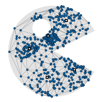
Figure 3: Exemplary constrained clustering instance of Section 3

We will now shortly discuss appropriate choices for $\mathcal{D}$ and $h$ and illustrate them by a simple example. In particular, we show how these choices relate to clusterings with certain characteristics.

An example

Figure 3 shows an instance of constrained geometric clustering. Here, the space $\mathcal{X}$ (gray filled area) is a subset of $\mathbb{R}^{2}$ that is not simply connected. The set $X$ consists of $500$ points (blue dots), each of weight $1$. We want to find a clustering of $k=5$ clusters, each of weight $100$. Also, a “distance graph“ $G$ (black lines) is given whose edges are weighted by the Euclidean distances of their nodes. For this example, $G$ was constructed via a Delaunay triangulation of $X$ and dropping edges outside $\mathcal{X}$. This graph encodes an intrinsic connectivity structure for $X$. Finally, the black-framed white squares depict the sites $\mathcal{S}$, which we assume to be pre-determined in this example. Figures 5 to 9 show the clusterings and supporting diagrams obtained for the different choices of $\mathcal{D}$ and $h$ via the methodology described above.

3.1 Euclidean Space

First, we consider the case that all metrics in $\mathcal{D}$ are Euclidean.

Additively Weighted Voronoi Diagrams

An obvious choice is $h=\operatorname{id}$, i. e., $f_{i}(x):=||x-s_{i}||+\mu_{i}$ is the Euclidean distance to the respective cluster’s site shifted by $\mu_{i}$. Solving (P) for a general instance then means to search for a fractional clustering minimizing the weighted average Euclidean distance to the assigned sites. All clusterings in the relative interior of the optimal face of (P) are supported by additively weighted Voronoi diagrams. For results on the latter see [4], [50, Chapter 3.1.2], [7, Chapter 7.4]. Here, Voronoi regions are separated by straight lines or hyperbolic curves and are in particular star-shaped w. r. t. their respective sites; see Figure 5. If $\mathcal{X}$ is convex, this yields connected regions. Of course, as the above example shows, this does not hold for general $\mathcal{X}$.

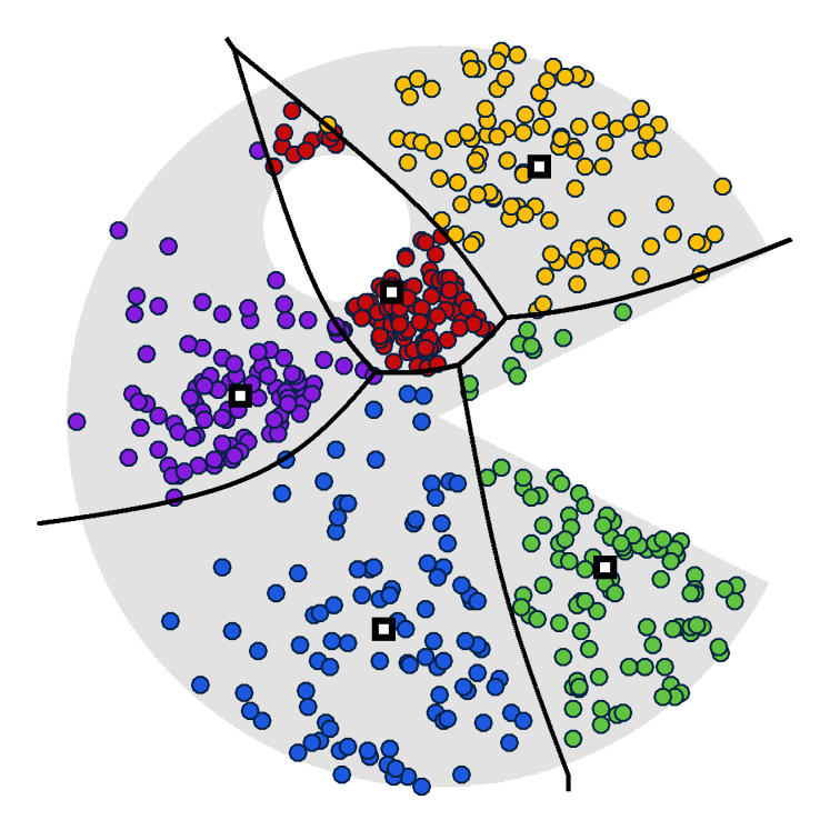
Figure 4: Clustering w. r. t. $\hat{f}_{i}(x)=||s_{i}-x||$

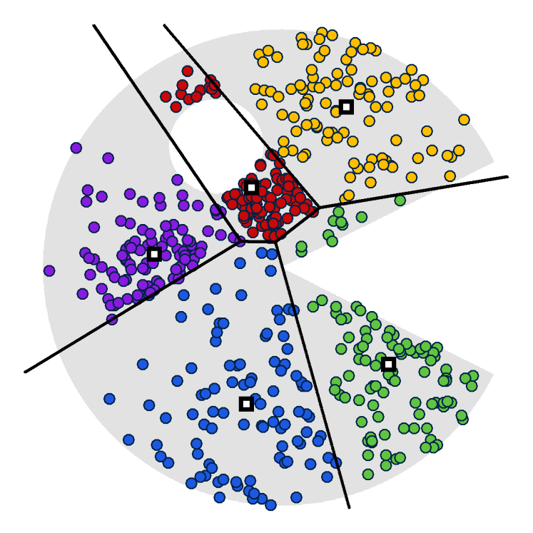
Figure 5: Clustering w. r. t. $\hat{f}_{i}(x)=||s_{i}-x||^{2}$

Power Diagrams

Taking the squared Euclidean distances, i. e., $f_{i}(x):=||x-s_{i}||^{2}+\mu_{i}$, yields power diagrams (see [6], [50, Chapter 3.1.4]). Figure 5 shows this case for our example. Here, regions are separated by straight lines perpendicular to the line spanned by the respective sites. In particular, this yields convex and therefore connected regions whenever $\mathcal{X}$ is a convex subset of $\mathbb{R}^{n}$. Again, connectivity might get lost when $\mathcal{X}$ is non-convex as is the case in this example. Solving (P) may be interpreted as minimizing the weighted squared error when the clusters are represented by their respective sites.

As already pointed out, power diagrams have been thoroughly investigated for the example of farmland consolidation ([13], [11]) and a comprehensive theory on their algorithmic treatment has been derived ([15], [14], [9]).

Let us close this subsection by briefly recapitulating a result from [15] that deals with optimal choices of the sites in the strongly balanced case. Recall that a feasible power diagram is called centroidal if

$$s_{i}=c(C_{i}):=\frac{1}{\kappa_{i}}\sum_{j=1}^{m}\xi_{i,j}\omega_{j}x_{j}$$

for $i=1,\ldots,k$. The following result characterizes centroidal power diagrams as local maximizers of the function $\phi:\operatorname{BC}\rightarrow\mathbb{R}$ defined by

$$\phi(\mathcal{C}):=\sum_{i=1}^{k}\kappa_{i}||c(C_{i})||^{2}.$$

Here, some trivial cases of clusters have to be excluded: A clustering $\mathcal{C}\in\operatorname{BC}$ is called proper, if for all $i\neq l$ it holds that

$$|\operatorname{supp}(C_{i})|=|\operatorname{supp}(C_{l})|=1\Rightarrow\operatorname{supp}(C_{i})\neq\operatorname{supp}(C_{l}).$$

Theorem 9 ([15, Theorem 2.4]).

Let $\mathcal{C}\in\operatorname{BC}$ be proper. Then there exists a centroidal power diagram that supports $\mathcal{C}$ if and only if $\mathcal{C}$ is the unique optimum of (P) and a local maximizer of $\phi$.

Furthermore, finding the global maximum of $\phi$ over $\operatorname{BC}$ is equivalent to optimizing

$$\min_{\mathcal{C}\in\operatorname{BC}}\sum_{i=1}^{k}\sum_{j=1}^{m}\xi_{i,j}\omega_{j}||x_{j}-c(C_{i})||^{2}.$$ (6)

This may be read as minimizing an average variance of clusters, also called the moment of inertia.

Note that $\phi$ actually depends only on the centers of gravity rather than on the clusters themselves. By definition those centers are given by a linear transformation of $\operatorname{BC}$ into the set of all gravity centers in $\mathbb{R}^{kd}$. Optimizing $\phi$ over $\operatorname{BC}$ is then equivalent to maximizing an ellipsoidal norm in $\mathbb{R}^{kd}$ over the set of gravity centers. One can now approximate this norm in the comparably low dimensional space $\mathbb{R}^{kd}$ by a polyhedral norm. This yields an approximation algorithm by solving a typically manageable number of linear programs of type (P); see [14], [15].

Another possibility to derive local optima of $\phi$ is by means of a balanced variant of the k-means algorithm (see [9]).

3.2 Anisotropic Diagrams with Ellipsoidal Norms

Using the Euclidean norm obviously cannot pay regard to the shape of $\mathcal{X}$ nor any other information about the desired extents or orientations of the resulting clusters. One possibility of including such information is to use anisotropic diagrams.

While we could, in principle, employ arbitrary norms we will consider $\mathcal{D}$ to be induced by ellipsoidal norms in the following. So, let $M_{i}\in\mathbb{R}^{n\times n}$ be symmetric positive definite matrices defining the ellipsoidal norms via

$$||x||_{M_{i}}:=\sqrt{x^{\text{\tiny T}}M_{i}x},$$

$i=1,\ldots,k$. In our main application, the matrices are chosen so as to obtain clusters similar to a pre-existing structure (cf. Section 4.4).

As in the Euclidean case, we consider the transformation functions $h=\operatorname{id}$ and $h=(\cdot)^{2}$. For $h=\operatorname{id}$ we obtain anisotropic Voronoi diagrams. These have already been applied in the field of mesh generation ([42], [18]) on a Riemannian manifold in $\mathbb{R}^{n}$ provided with a metric tensor $M:\mathcal{X}\rightarrow M^{n\times n}$. Hence, the functions $f_{i}$ can be seen as local approximations of the geodesic distances w. r. t. that manifold. Even without additive weights, the resulting diagrams need not be connected.

We will refer to case $h=(\cdot)^{2}$ as anisotropic power diagrams. In [1] these were successfully used for the reconstruction of polycrystalline structures, where information about volumes as well as moments of crystals is given. Regions are separated by straight lines or quadratic curves. Figures 7 and 7 show the case of additively weighted anisotropic Voronoi diagrams and anisotropic power diagrams, respectively. The dotted ellipses depict the unit balls of the respective norms.

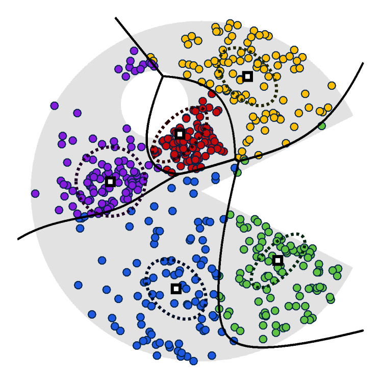
Figure 6: Clustering w. r. t. $\hat{f}_{i}(x)=\sqrt{(x\!-\!s_{i})^{\text{\tiny T}}M_{i}(x\!-\!s_{i})}$

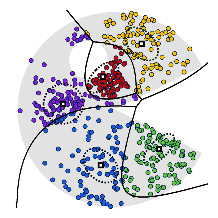
Figure 7: Clustering w. r. t. $\hat{f}_{i}(x)=(x\!-\!s_{i})^{\text{\tiny T}}M_{i}(x\!-\!s_{i})$

3.3 Shortest-Path Diagrams

Even in the anisotropic case, the diagrams considered so far might fail in depicting intrinsic relations of the points in $\mathcal{X}$. In our application of electoral district design, this occurs as points are only representatives of their municipalities’ regions. Thus, information about neighborhood relations is lost (cf. Section 4). In such cases, generalized Voronoi diagrams on an edge-weighted graph $G=(X,E,\delta)$ can be preferable.

Figure 9 shows the result if $\mathcal{X}$ is the discrete space of all elements in $X$ together with the metric induced by $G$ (see Section 1). Taking $f_{i}(x):=d_{G}(s_{i},x)+\mu_{i}$, this means that the weighted average distance of elements to their assigned sites in the graph is minimized. We will refer to this case as shortest-path diagrams. Of course, if $G$ is complete and edge weights are the Euclidean distances between the vertices, this again results in additively weighted Voronoi diagrams.

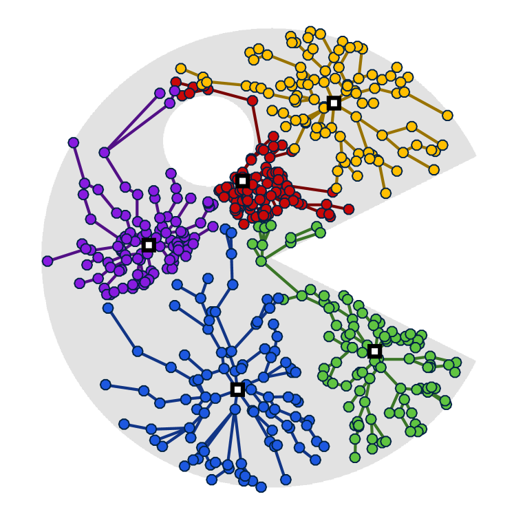
Figure 8: Clustering w. r. t. $\hat{f}_{i}(x)=d_{G}(s_{i},x)$

Figure 9: Clustering w. r. t. $\hat{f}_{i}(x)=d_{G}(s_{i},x)^{2}$

In general, there are two main motivations to use a discrete space $(X,d_{G})$. The obvious first reason are applications that live on some sort of graph. For instance, [49] proposes to use Voronoi diagrams on discrete spaces for the representation of service areas in cities as the Euclidean norm is often unsuitable for approximating distances in urban traffic networks. Second, there are applications that require clusters to be connected in some sense. Often, of course, this connectivity is already established when clusters are supported by a diagram in $\mathcal{X}$ with connected regions. However, as has been observed before, this is not always the case with the diagrams proposed so far, in particular, since the underlying space might not be convex.

We say that a fractional clustering $\mathcal{C}\in\operatorname{BC}$ is $\mathcal{S}$-star-shaped for sites $\mathcal{S}=\left(s_{1},\ldots,s_{k}\right)\in X^{k}$, if for every $i\in\{1,\ldots,k\}$ and $x\in\operatorname{supp}(C_{i})$ it follows that $v\in\operatorname{supp}(C_{i})$ for every $v$ on a shortest $s_{i}$-$x$-path in $G$. By the following result, clusters that are supported by shortest-path diagrams are $\mathcal{S}$-star-shaped. More precisely, the Voronoi regions are shortest-path trees rooted at their sites.

Theorem 10.

Let $(X,d_{G})$ be the metric space induced by a connected and edge-weighted graph $G=(X,E,\delta)$. Let $\mathcal{C}\in\operatorname{BC}$, $\mathcal{S}\in X^{k}$, $\mathcal{M}\in\mathbb{R}^{k}$, and define $\mathcal{D}:=\left(d_{1},\ldots,d_{k}\right)$ via $d_{i}=d_{G}$ for $i=1,\ldots,k$.

If the generalized Voronoi diagram $\mathcal{P}$ w. r. t. $\mathcal{F}(\mathcal{D},{\operatorname{id}},\mathcal{S},\mathcal{M})$ supports $\mathcal{C}$, then $\mathcal{C}$ is $\mathcal{S}$-star-shaped. In particular, $s_{i}\in\operatorname{supp}(C_{i})$ holds for all $i\in\{1,\ldots,k\}$.

Proof.

Let $F$ be the optimal face of (P), then $\mathcal{C}\in\operatorname{relint}(F)$ holds by Corollary 3. For some $i\in\{1,\ldots,k\}$, let $x_{j}\in\operatorname{supp}(C_{i})$ and let $s_{i}=v_{1},v_{2},\ldots,v_{t}:=x_{j}$ be a shortest $s_{i}$-$x_{j}$-path in $G$.

Suppose that there exists $x_{p}$ such that $v_{l}=x_{p}\not\in\operatorname{supp}(C_{i})$ for some $l\in\{1,\ldots,t-1\}$. By the feasibility of $\mathcal{C}$ there exists $r\in\{1,\ldots,k\}$ such that $x_{p}\in\operatorname{supp}(C_{r})$.

Due to the choice of $x_{p}$ and $x_{j}$ it follows that $\xi_{i,p}=0<1$, $\xi_{i,j}>0$, $\xi_{r,j}\leq 1-\xi_{i,j}<1$ and $\xi_{r,p}>0$.

Let $\mathcal{Z}\in\mathbb{R}^{k\times m}$ be the cyclic exchange for the sequence $(i,x_{j},r,x_{p})$ (as defined in Section 2.3). Then there exists some $\alpha>0$ such that $\mathcal{C}+\alpha\mathcal{Z}\in\operatorname{BC}$. If $\alpha$ is sufficiently small $\mathcal{C}+\alpha\mathcal{Z}$ has (at least) one non-zero component more than $\mathcal{C}$. Since $\mathcal{C}\in\operatorname{relint}(F)$, it follows that $\mathcal{C}+\alpha\mathcal{Z}\not\in F$. Thus, $0<d_{G}(s_{i},x_{p})-d_{G}(s_{i},x_{j})+d_{G}(s_{r},x_{j})-d_{G}(s_{r},x_{p})$.

Now, by the triangle inequality, $d_{G}(s_{r},x_{j})\leq d_{G}(s_{r},x_{p})+d_{G}(x_{p},x_{j})$. As $x_{p}$ lies on a shortest $s_{i}$-$x_{j}$-path, it furthermore holds that $d_{G}(s_{i},x_{j})=d_{G}(s_{i},x_{p})+d_{G}(x_{p},x_{j})$.

Together, this yields $d_{G}(s_{r},x_{j})-d_{G}(s_{i},x_{j})\leq d_{G}(s_{r},x_{p})-d_{G}(s_{i},x_{p})$, a contradiction.

As $\operatorname{supp}(C_{i})\neq\emptyset$ for $i=1,\ldots,k$, this in particular implies $s_{i}\in\operatorname{supp}(C_{i})$. ∎

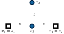
Figure 10: Intersecting shortest paths.

The requirement that $\mathcal{C}\in\operatorname{BC}$ lies in the relative interior of the optimal face (P) is crucial for shortest-path distances to preserve star-shapedness. In [59], a Lagrange relaxation model of an integer version of (P) for shortest-path distances was considered and connectivity of resulting clusters was demanded, while it was pointed out in [54], that this may not hold whenever non-unique optima appear. 10 clarifies the situation: in view of [54] it is precisely the requirement that the solution lies in the relative interior of the optimal set.

Let us now consider the example of Figure 10 with $a:=1,b:=1$, $c:=2$ and the resulting constrained clustering instance for $\Omega:=\mathds{1}$, $\mathcal{K}:=(2,2)^{\text{\tiny T}}$. We obtain the two clusterings $\mathcal{C}^{(a)}$, $\mathcal{C}^{(b)}\in\operatorname{BC}$ via

$$C^{(a)}_{1}:=(1,\frac{1}{2},\frac{1}{2},0),\hskip 20.00003ptC^{(a)}_{2}:=(0,\frac{1}{2},\frac{1}{2},1)$$

and

$$C^{(b)}_{1}:=(1,0,1,0),\hskip 20.00003ptC^{(b)}_{2}:=(0,1,0,1).$$

The generalized Voronoi diagram $\mathcal{P}^{\ast}$ w. r. t. $f_{1}(x)=d_{G}(s_{1},x)+1$ and $f_{2}(x)=d_{G}(s_{2},x)$ (i. e., $h={\operatorname{id}}$ and $\mathcal{M}=(1,0)^{\text{\tiny T}}$), consists of the cells $P^{\ast}_{1}=\{x_{1},x_{2},x_{3}\}$ and $P^{\ast}_{2}=\{x_{2},x_{3},x_{4}\}$. Thus, it is feasible for both $\mathcal{C}^{(a)}$ and $\mathcal{C}^{(b)}$. Hence, they are both minimizers of (P) by 1. However, only $\mathcal{C}^{(a)}$ is supported by $\mathcal{P}^{\ast}$ and $\mathcal{S}$-star-shaped while $\mathcal{C}^{(b)}$ contains a disconnected cluster.

More generally, this happens whenever shortest paths intersect. This can have a dramatic effect on integer assignments. In fact, in order to conserve connectivity after rounding, whole fractionally assigned branches of the shortest-path trees might have to be assigned to one of their supporting clusters. Of course, this results in greater deviations of cluster weights. For our running example, Figure 11 depicts the points that have originally been fractionally assigned to both the blue and the green colored cluster and are now fully assigned to the green cluster in the integer solution.

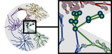
Figure 11: Rounded units in the case $\hat{f}_{i}(x)=d_{G}(s_{i},x)$.

Figure 12: Non-connected cluster in the case $\hat{f}_{i}(x)=d_{G}(s_{i},x)^{2}$.

A natural idea to overcome this effect as well as to obtain more consolidated clusters is to try to imitate the idea of squaring the distances (that led to power diagrams in the Euclidean space) to the discrete space $(X,d_{G})$.

Let us once more consider the previous example from just above. This time, however, we take the generalized Voronoi diagram $\mathcal{P}^{\prime}$ w. r. t. $f_{1}(x)=d_{G}(s_{1},x)^{2}+4$ and $f_{2}(x)=d_{G}(s_{2},x)^{2}$ (i. e., $h=(\cdot)^{2}$ and $\mathcal{M}=(4,0)^{\text{\tiny T}}$). It follows that $P^{\prime}_{1}=\{x_{1},x_{3}\}$ and $P^{\prime}_{2}=\{x_{2},x_{4}\}$. Thus, $\mathcal{P}^{\prime}$ supports $\mathcal{C}^{(b)}$ but is not even feasible for $\mathcal{C}^{(a)}$. In fact, $\mathcal{C}^{(b)}$ is the unique minimizer of (P) for this choice of $h$ and does not yield connected clusters. Figure 12 demonstrates the same effect for our running example. Here, the single yellow unit in the center is separated from its respective cluster.

Unfortunately, the following theorem shows that this is a general effect. In fact, for any transformation function $h$ that is not affine, clusters can be disconnected despite being supported by a corresponding diagram. Thus, if connectivity is to be guaranteed a-priorily, this dictates the choice of shortest-path diagrams in our approach.

Theorem 11.

Let $(X,d_{G})$ be the metric space induced by a connected and edge-weighted graph $G$. Let $\mathcal{C}\in\operatorname{BC}$, $\mathcal{S}\in X^{k}$, and $\mathcal{M}\in\mathbb{R}^{k}$, and define $\mathcal{D}=\left(d_{1},\ldots,d_{k}\right)$ via $d_{i}=d_{G}$ for $i=1,\ldots,k$. Furthermore, let $h:\mathbb{R}_{\geq 0}\rightarrow\mathbb{R}$ be continuous.

If $h(x)=\alpha\cdot x+\beta$ for some $\alpha\in\mathbb{R}_{\geq 0},\beta\in\mathbb{R}$ and the generalized Voronoi diagram w. r. t. $\mathcal{F}(\mathcal{D},h,\mathcal{S},\mathcal{M})$ supports $\mathcal{C}$, then $\mathcal{C}$ is $\mathcal{S}$-star-shaped.

If $h$ is any continuous function but not of the above type, this is not true in general.

Proof.

The first claim follows by replacing $d_{G}$ with $\alpha\cdot d_{G}+\beta$ in the proof of 10. Note that in the case $\alpha=0$ the whole set $\operatorname{BC}$ is optimal, which causes all components of a solution from the relative interior to be strictly positive.

For the second claim, let some continuous function $h:\mathbb{R}_{\geq 0}\rightarrow\mathbb{R}$ be given. Consider the graph from Figure 10 with $X=\{x_{1},x_{2},x_{3},x_{4}\}$, edges $\{\{x_{1},x_{2}\}$, $\{x_{2},x_{3}\}$, $\{x_{2},x_{4}\}\}$ and edge weights $\delta(\{x_{1},x_{2}\})=a$, $\delta(\{x_{2},x_{3}\})=b$ and $\delta(\{x_{2},x_{4}\})=c$ for some $a,b,c\in\mathbb{R}_{>0}$. Furthermore, let $\omega_{1}=\omega_{2}=\omega_{4}=1$, $\omega_{3}=3$ and $\kappa_{1}=\kappa_{2}=3$. By Corollary 3 and since $\operatorname{BC}\neq\emptyset$ there exists a clustering $\mathcal{C}\in\operatorname{BC}$ that is supported by the generalized Voronoi diagram $\mathcal{P}$ w. r. t. $\mathcal{F}(\mathcal{D},h,\mathcal{S},\mathcal{M})$ for some $\mathcal{M}\in\mathbb{R}^{2}$.

Now suppose that $\mathcal{C}$ is $\mathcal{S}$-star-shaped. Together with the choice of the weights this implies $\{x_{2},x_{3}\}\subset\operatorname{supp}(C_{1})\cap\operatorname{supp}(C_{2})\subset P_{1}\cap P_{2}$. Hence, one gets $h(d_{G}(s_{1},x_{j}))+\mu_{1}=h(d_{G}(s_{2},x_{j}))+\mu_{2}$ for $j=2,3$. Subtraction of the equality for $j=3$ from the one for $j=2$ and insertion of the shortest paths lengths yields

$$h(a)-h(a+b)=h(c)-h(c+b).$$

Setting $\tilde{h}:=h-h(0)$, taking the limit $c\rightarrow 0$ and using the continuity of $h$ this implies

$$\tilde{h}(a+b)=\tilde{h}(a)+\tilde{h}(b).$$

Since $a,b\in\mathbb{R}_{>0}$ are arbitrary and $\tilde{h}$ is continuous, it readily follows that $\tilde{h}$ is linear on $\mathbb{R}_{\geq 0}$ and thus $h$ is of the form $h(t)=\alpha\cdot t+\beta$.

In order to see that $\alpha\geq 0$, it is sufficient to consider the example $X=\{x_{1},x_{2}\}$, $s_{i}=x_{i},\omega_{i}=1,\kappa_{i}=1$ for $i=1,2$ and a single edge $\{x_{1},x_{2}\}$ of arbitrary positive length. If $\alpha<0$, then the optimal clustering is $\operatorname{supp}(C_{1})=\{x_{2}\}$ and $\operatorname{supp}(C_{2})=\{x_{1}\}$, which contradicts the claim of 10. ∎

4 Application to the Electoral District Design Problem

We will now apply our approach to the electoral district design problem. We show the effect of using power diagrams, anisotropic power diagrams and shortest-path diagrams for the example of the Federal Republic of Germany.

4.1 Electoral District Design

Despite the differences in voting systems, the issue of designing electoral districts can be stated in a common way suitable for most of them. A state consists of basic units such as municipalities or smaller juridical entities. Units are of different weight, usually and in the following their number of eligible voters. Units are then to be partitioned into a given number of districts of (approximately) equal weight. Hence, we are facing a constrained clustering problem as defined in Section 2.1.

Usually, districts are required to be “compact” and “contiguous” (cf. [51]). Both are, not formally defined juridical demands requiring a proper mathematical modelling. How to define a measure for “compactness” of districts has, in fact, been widely discussed in the literature (e. g. [58], [47], [35], [2]). One widely accepted measure ([33], [28]) is the moment of inertia as defined by (6), where each municipality is modelled as a point in the Euclidean plane.

Contiguity usually requires that the area belonging to a district’s municipalities is connected. This can be modelled by the adjacency graph $G$ with nodes corresponding to the units and edges between two units whenever they share a common border (which can be crossed). Connectivity of clusters is then defined by demanding that each induced subgraph $G[\operatorname{supp}(C_{i})]$ is connected. The edges of $G$ can be weighted, for example, by driving distances between the corresponding municipalities’ centers.

Due to census development electoral districts have to be regularly adapted. Therefore, a further requirement may be to design districts that are similar to the existing ones. Let $\mathcal{C}^{\text{o}}$ be the integer clustering that corresponds to the original districts and $\mathcal{C}^{\ast}$ be a newly created integer clustering. One may measure the difference of the two district plans by the ratio of voter pairs that used to share a common district but are now assigned to different ones. With $A(\mathcal{C}^{\text{o}},\mathcal{C}^{\ast}):=\{(j,r):1\leq j<r\leq m\wedge\exists i:\xi^{\text{o}}_{i,j}=\xi^{\text{o}}_{i,r}=1~{}\wedge\forall i:\xi^{\ast}_{i,j}\cdot\xi^{\ast}_{i,r}=0\}$ this is, more formally, given by

$$\frac{1}{\sum_{i=1}^{k}\tbinom{\omega(C^{\text{o}}_{i})}{2}}\sum_{(j,r)\in A(\mathcal{C}^{\text{o}},\mathcal{C}^{\ast})}\omega_{j}\cdot\omega_{r}.$$ (7)

4.2 Dataset Description

By the German electoral law [25], there are a total of 299 electoral districts that are apportioned to the federal states according to their population. As districts do not cross state borders, each state must be considered independently. A district’s size is measured by its number of eligible voters ([24]). It should not deviate from the federal average by more than 15%; a deviation exceeding 25% enforces a redesign of districts. As far as possible, for administrative and technical reasons municipal borders must be conserved. Furthermore, districts are supposed to yield connected areas.

For our application the data from the last German election held on September 22nd 2013 was used. Statistics about the number of eligible voters were taken from [26]. Geographic data for the municipalities and election districts of 2013 were taken from [23] and [27], respectively. Greater cities which on their own constituted one or several election districts in 2013 were neglected for our computations as any proper district redesign would imply to split these municipalities up into smaller units and thus, of course, required data on a more granular basis. For the same reason, the city states (Berlin, Bremen, Hamburg) were not taken into consideration.

Figure 1(a) depicts the deviation of clusters sizes of the 2013 election from the federal average. Accordingly, in the 2013 elections 57 of the 249 districts that were considered had a deviation of more than 15%. The overall average deviation is 9.5%. The maximum deviation of 25.15% is obtained for a district in the state of Bavaria.

We have identified each municipality by a point in the plane given by its geographic coordinates in the EPSG 3044 spatial reference system ([57]). For the shortest-path clustering approach, we have an edge in the graph $G$ between two municipalities whenever their regions share a border. The edge lengths were taken as driving distances obtained from the MapQuest Open Geocoding API ([43]).

In the following of this chapter, we state the practical results for all of Germany and for various single states. The latter are typical examples, i. e., the individual results for the other states are very similar; see Appendix A and http://www-m9.ma.tum.de/material/districting/.

4.3 Power Diagrams

As pointed out in Section 3.1, clusterings with minimal moment of inertia are supported by centroidal power diagrams. Thus, power diagrams yield highly consolidated district plans.

Squared Euclidean distances were already used for the problem of electoral district design; see e.g. [33] and [34]. Centroidal power diagrams have been used by [28], who presented a gradient descent procedure similar in spirit to the balanced $k$-means approach ([9]).

In our approach, first a fractional clustering that is supported by a centroidal power diagram was created. Here, the sites were determined as approximations of the global optimizers of (6) as proposed in [14]. Second, the fractionally assigned units were rounded optimally with respect to the resulting balancing error.

As it turns out, non-connected districts do indeed sometimes occur. This is due to the non-convexity of the states in general and particularly due to “holes” in the state areas resulting from excluded municipalities or city states. In many cases, this may not regarded a problem. However, since we insisted on connected districts we applied some post-processing. After running the approach as described in Section 3.1, the resulting districts were checked for connectivity. This was done in an automated manner using the adjacency graph of neighboring units and standard graph algorithms. If unconnected districts were detected, the program (P) was rerun under preventing or forcing municipalities to be assigned to a certain district by constraining the corresponding decision variables to 0 or 1, respectively. For example, if a district had been split into two parts by a geographical barrier such as a lake or an indentation in the state border, the smaller part (which mostly consisted of a a single municipality) was excluded from being assigned to that district. This was comfortably done using a graphical user interface and required only a few, if any, iterations per state. For the considered data, a total of 51 (0.46%) municipalities was preassigned in order to establish connectivity.

Figure 13 shows the original districts of the state of Bavaria from the 2013 elections compared to the results of the power diagram approach. Figure 13(b) furthermore depicts the resulting polyhedral power diagram regions. Here, three units had to be fixed in order to establish connectivity.

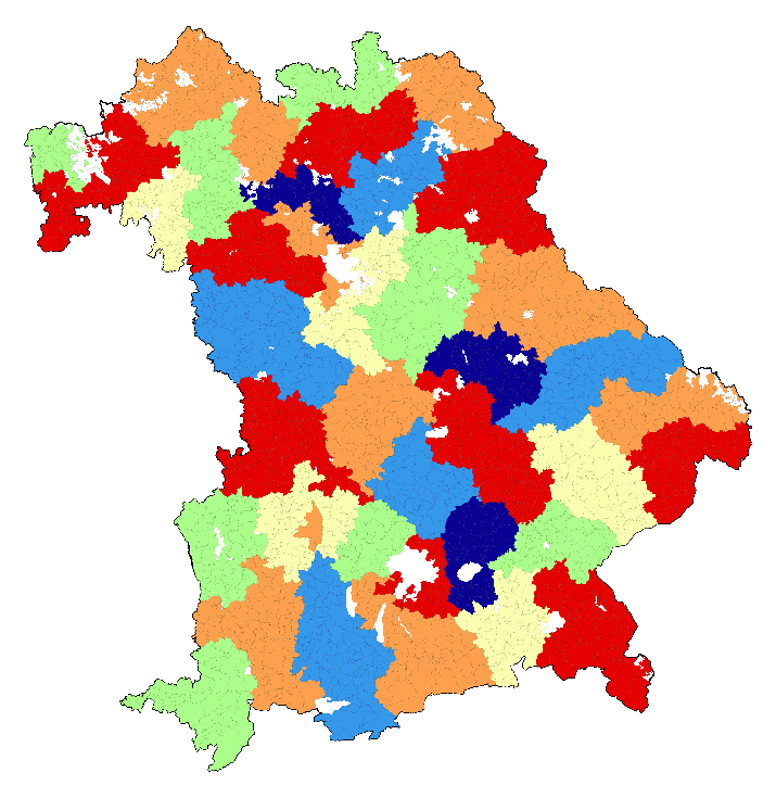
(a) Districts from the 2013 elections.

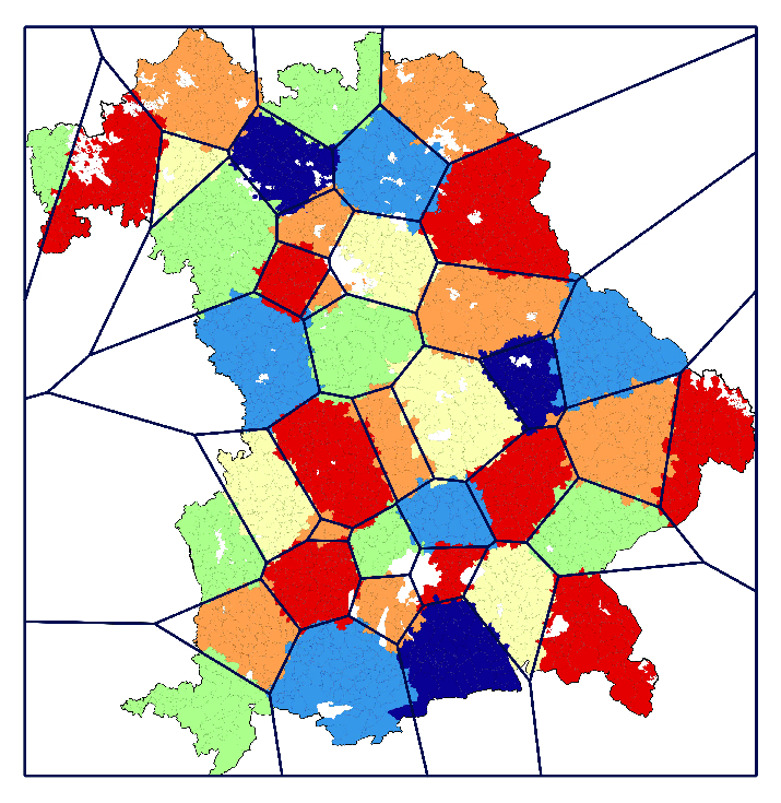
(b) Districts via power diagrams.

Figure 13: Districts for the state of Bavaria. Here and in the following, we use a six-coloring of the districts for an easy distinguishability.

4.4 Anisotropic Power Diagrams

Next, we show how to use anisotropic power diagrams in order to obtain clusters that are similar to those of the 2013 election.

As in [1], a principal component analysis was performed in order to determine a local ellipsoidal norm for each district. Let $\mathcal{C}^{\text{o}}:=\left(\xi^{\text{o}}_{i,j}\right)_{\begin{subarray}{c}i=1,\ldots,k\\ j=1,\ldots,m\end{subarray}}$ be the integer clustering encoding the original districts of some state. For each $i=1,\ldots,k$, the covariance matrix $V_{i}$ is computed as

$$V_{i}:=\sum_{j=1}^{m}\frac{\xi^{\text{o}}_{i,j}\omega_{j}}{\omega(C^{\text{o}}_{i})}\left(x_{j}-c(C^{\text{o}}_{i})\right)\left(x_{j}-c(C^{\text{o}}_{i})\right)^{\text{\tiny T}}.$$

Using a singular value decomposition, we obtain an orthogonal matrix $Q\in\operatorname{O}(2)$ and $\sigma_{1}^{(i)},\sigma_{2}^{(i)}>0$ such that

$$V_{i}=Q\begin{pmatrix}\sigma_{1}^{(i)}&0\\ 0&\sigma_{2}^{(i)}\end{pmatrix}Q^{\text{\tiny T}}.$$

We then set

$$M_{i}:=Q\begin{pmatrix}(\sigma_{1}^{(i)})^{-1}&0\\ 0&(\sigma_{2}^{(i)})^{-1}\end{pmatrix}Q^{\text{\tiny T}}$$

in order to obtain an ellipsoidal norm as described in Section 3.1. With the centroids of $\mathcal{C}^{\text{o}}$ as starting sites we performed a balanced k-means algorithm (see [9]) in order to obtain centroidal anisotropic power diagrams.

As in the case of power diagrams and due to the same reasons, again not all of the resulting clusters were connected. Applying the same post-processing this could again be treated, affecting a total of 33 (0.30%) municipalities.

Figure 14 shows the 2013 elections’ districts of the state of Lower Saxony and the results of the anisotropic power diagram approach. The blue ellipses in 14(b) depict the unit balls of corresponding local cluster norms. For this state no post-processing was necessary.

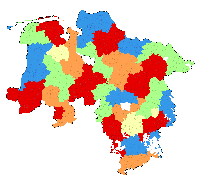
(a) Districts from the 2013 election.

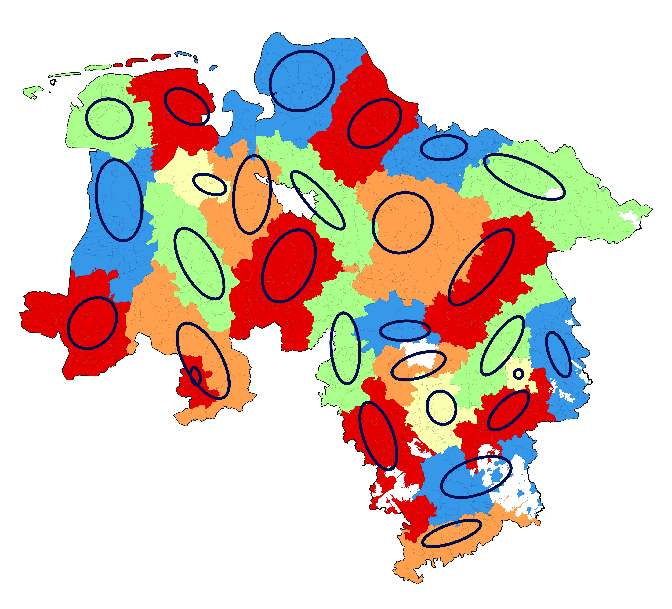
(b) Districts via anisotropic power diagrams. Ellipses depict unit balls of local norms (determined from the districts of 2013).

Figure 14: Districts for the state of Lower Saxony.

4.5 Shortest-Path Diagrams

In order to enforce connectivity directly, we apply the shortest-path diagrams of Section 3.3 w. r. t. the adjacency graph $G$ of neighboring units. Shortest-path distances have appeared in the context of electoral district design several times (e. g., [55], [59], [54], [39], [53]). In [52] also Voronoi diagrams on a connectivity graph were considered but multiplicative rather than additive weights were evoked, which led to substantially bigger balancing errors. In [59] and [54], Lagrangian relaxations were applied which are, naturally, closely related to our methodology.

In our approach, the effect of non-unique optima and therefore more fractionality could be observed as predicted in Section 3.3. This was again handled in a post-processing phase by the implementation of a slightly more sophisticated rounding procedure. Here, fractional components were rounded in an iterative manner while updating the shortest-path distances to the already integrally assigned clusters in each step. In order to determine suitable sites $s_{i}$, $i=1,\ldots,k$, a simple local search w. r. t. improvement of the resulting deviation of cluster sizes was performed. Here, the units closest to the centroids of $\mathcal{C}^{\text{o}}$ served as starting sites.

Figure 15 shows the original districts of the state of North Rhine-Westphalia from the 2013 elections compared to the results via shortest-path diagrams. The edges in Figure 15(b) furthermore depict the shortest-path trees connecting the resulting clusters.

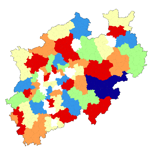
(a) Districts from the 2013 election.

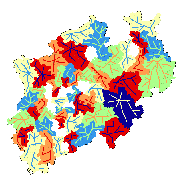
(b) Districts via shortest-path diagrams.

Figure 15: Districts for the state of North Rhine-Westphalia.

4.6 Evaluation

We will now summarize the results of our different approaches. See Appendix A in the appendix for a more detailed overview of the results for the different German states.

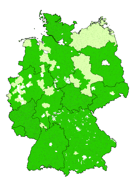
(a) Power diagram approach.

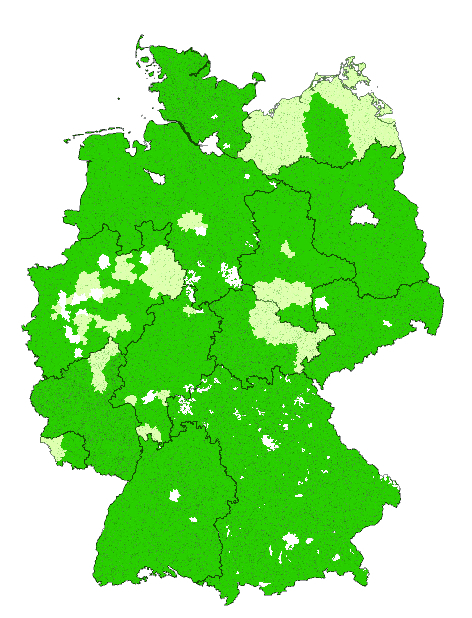
(b) Anisotropic power diagram approach.

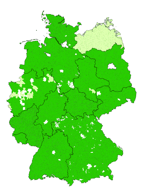
(c) Shortest-path diagram approach.

Figure 16: Deviations after applying our methodology. Colors as in Figure 1.

As already pointed out, all approaches led to district plans complying with the German electoral law, i. e. obeying the deviation limits and connectivity of districts.

	Districts 2013	Power Diagrams	Anisotropic Power Diagrams	Shortest-Path Diagrams
Avg.	9.52%	2.69%	2.73%	2.13%
Max.	25.1%	10.60%	14.71%	9.73%

Table 1: Deviations of district sizes from the federal average size.

The largest maximal deviations occur for the states of Mecklenburg-Vorpommern (14.71%) and North Rhine-Westphalia (14.34%), both for the anisotropic power diagram approach. However, Appendix A shows that even those deviations are not far off from optimality. In fact, the average district size in Mecklenburg-Vorpommern itself is already 8.9% below the federal average. In North Rhine-Westphalia, the high population density results in units of greater weight and thus greater rounding errors. As expected, Appendix A shows that states with a finer division into municipalities generally yield smaller deviations.

Figure 16 depicts the deviations of district sizes for our approaches and Table 1 contains the average and maximal values for all our approaches and the elections of 2013. While all approaches perform well, the shortest-path diagram approach is slightly superior. This is not surprising, as the local search in the shortest-path approach only focuses on the deviation error.

	Power Diagrams	Anisotropic Power Diagrams	Shortest-Path Diagrams
$\Delta$MoI	-11.3%	1.3%	-0.5%

Table 2: Relative change of the moment of inertia as defined by (6) compared to 2013.

Table 2 yields the relative change of the total moment of inertia (as defined in (6)) compared to 2013. According to this measure, power diagrams lead to the by far best consolidation. Shortest-path diagrams yield slightly more and the anisotropic power-diagram slightly less consolidated districts. However, recall that the moment of inertia is measured in Euclidean space, while the anisotropic power diagrams minimize local ellipsoidal norms. Hence, a fair comparison should really involve a measure similar to (6) but based on those local norms.

	Power Diagrams	Anisotropic Power Diagrams	Shortest-Path Diagrams
$\Delta$Pairs	40.6%	21.4%	35.4%

Table 3: Total ratio of changed pairs of voters as defined by (7).

In order to compare the obtained districts to the ones of 2013, the ratio of changed pairs according to (7) over the districts of all states are shown in Table 3. Here, indeed the anisotropic power diagram approach separates significantly less pairs of voters that used to vote in the same district in the 2013 election.

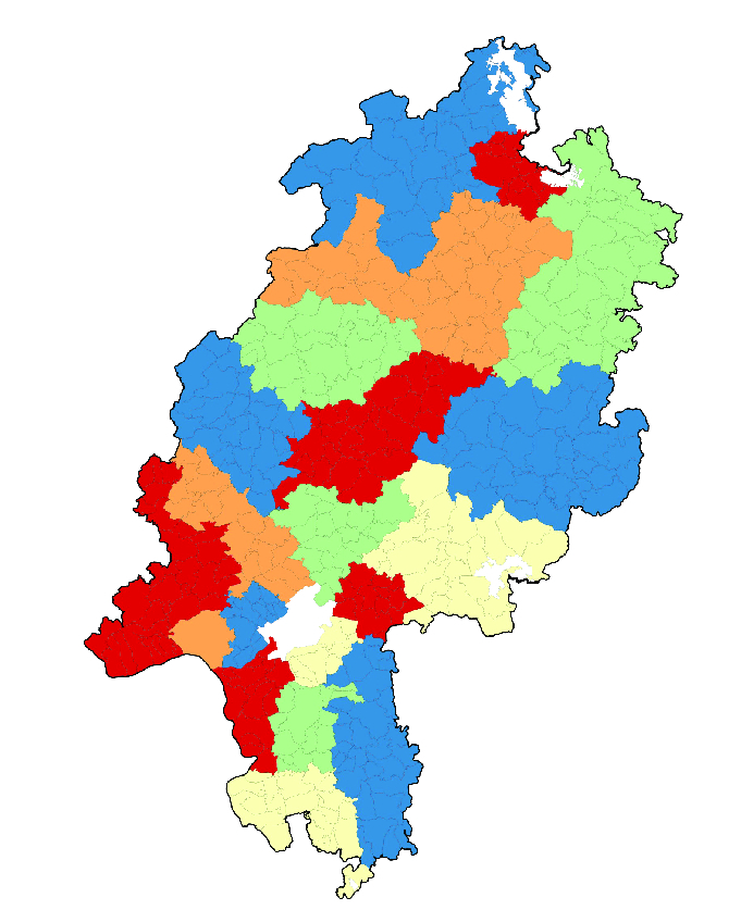
(a) Original districts of the 2013 election.

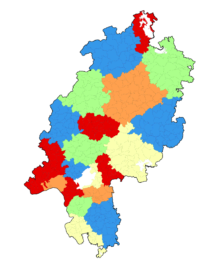
(b) Districts via power diagrams.

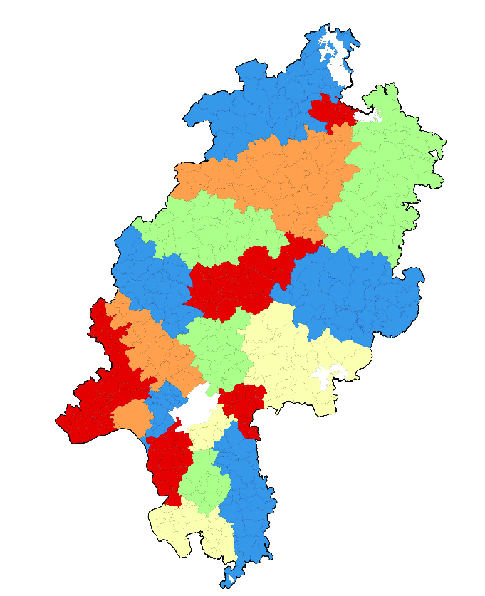
(c) Districts via anisotropic power diagrams.

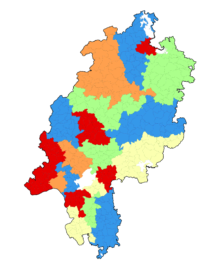
(d) Districts via shortest-path diagrams.

Figure 17: Districts for the state of Hesse resulting from the different approaches. See also Appendix A for corresponding key figures.

Figure 17 shows the results of the state of Hesse for all approaches in direct comparison. In particular, they illustrate the numbers listed above. The power diagram districts seem most consolidated, while elongated districts appear in the shortest-path result. Also, a higher degree of similarity of the districts from anisotropic power diagrams to the original districts can be recognized.

Finally, concerning the computational running times of our approaches, note that once the parameters $(\mathcal{D},h,\mathcal{S})$ are determined, a simple linear program (P) in dimension $k\times m$ with $k+m$ constraints and $2km$ non-zero entries is to be solved. This, of course, is unproblematic even for fairly large instances (such as, for example, $10^{5}$ municipalities and $10^{3}$ districts) using state-of-the-art solvers.

When, however, the structural parameters are part of the optimization process, the computational scalability strongly depends on the chosen approach: In case of power diagrams, an approximate optimization of (6) (cf. Section 3.1) also leads to solving a number of linear programs in dimension $k\times d$ and a fairly small number of constraints. However, this means approximately maximizing an ellipsoidal norm, which is an ${\mathcal{NP}}$-hard problem with no constant-factor approximation unless $\mathcal{P}={\mathcal{NP}}$ (cf. [16], [17], [12], [15]). Thus, this will be problematic for huge $k$. However, as the number of representatives is limited and, particularly, voting is in effect often restricted to subpopulations (like the states within the Federal Republic of Germany), this remains tractable in practice (as demonstrated).

In the case of anisotropic power diagrams, the applied balanced k-means variant reduces to solving (P) a few times.

As we applied a local-search of sites for shortest-path diagrams, there, the running times are, of course, highly dependent on the size of the considered neighborhoods that are evaluated. In our computations, we restricted a sites vector’s neighborhood to single site-exchanges with the respective 50 closest units. Then, if the local search is performed separately for each cluster, we can again expect good scalability in terms of $k$.

For our data sets, the computations ran on a standard PC within seconds for anisotropic power diagrams, within few hours for (approximately) centroidal power diagrams and were in the range of several hours for the shortest-path approach. In any case, for our application of electoral districting the computation times were not critical.

5 Conclusion

We presented a unifying approach to constrained geometric clustering in arbitrary metric spaces and applied three specifications to the electoral district design problem. We used a relation between constrained fractional clusterings and additively weighted generalized Voronoi diagrams which is based on LP-duality. In particular, we obtained clusterings with prescribed cluster sizes that are embeddable into additively weighted generalized Voronoi diagrams. A short discussion of typical classes of diagrams as well as details for the special cases of power diagrams and shortest-path diagrams on graphs were provided.

	Power Diagrams	Anisotropic Power Diagrams	Shortest-Path Diagrams
consolidation	$\oplus$ $\oplus$	$\oplus$
connectivity	$\oplus$		$\oplus$ $\oplus$
conservation of existing structure		$\oplus$ $\oplus$	$\oplus$

Table 4: ”rule of thumb” for the choice of diagram types

Results for the example of electoral district design in Germany prove to be very favorable with respect to the deviations from prescribed cluster sizes of the obtained integer clusterings. In particular, we pointed out how the choice of a class of diagrams can be made for the different optimization criteria. Table 4 summarizes our observations by providing an informal ”rule of thumb” for the choice of a diagram type: If particularly consolidated districts are desired, power diagrams yield the best results. As they further produce convex cells, the resulting districts are likely to be connected whenever the units can be approximated well by points in the plane and the state area is close to convex. If districts are preferred that are similar to existing structures, anisotropic power diagrams perform very well. Due to their relation to power diagrams, they have favorable characteristics w. r. t. consolidation as well. Connectivity is guaranteed a-priorily by shortest-path diagrams. Note that with edge distances obtained from anisotropic norms, conservation of existing structures may here be achieved, too. Thus, our methodology is capable of satisfying different requirements that may occur for political reasons.

Appendix A Results for the German federal election

				2013	Power Diagrams			Anisotropic Power Diagrams			Shortest-Path Diagrams
State	$m$	$k$	State Dev	øDev	øDev	$\Delta$MoI	$\Delta$Pairs	øDev	$\Delta$MoI	$\Delta$Pairs	øDev	$\Delta$MoI	$\Delta$Pairs
				in %	in %	in %	in %	in %	in %	in %	in %	in %	in %
Baden-Württemberg	1100	36	1.9	7.9	1.9	-13.1	41.0	2.1	0.6	21.3	1.9	0.9	35.2
Bavaria	2055	40	0.9	13.8	1.4	-14.8	44.5	1.2	4.3	37.0	0.9	2.7	44.1
Brandenburg	419	10	0.3	15.8	1.6	-7.5	29.5	1.7	4.8	21.0	0.3	-1.6	32.7
Hesse	425	20	3.5	9.1	3.6	-15.2	39.2	3.5	0.0	17.9	3.5	5.0	36.1
Mecklenburg-Vorpommern	780	6	8.7	8.9	8.7	-12.1	24.3	8.7	-6.4	15.3	8.7	-1.1	24.1
Lower Saxony	1001	28	1.0	7.8	2.4	-14.3	42.9	1.5	-3.1	18.5	1.1	-8.9	39.9
North Rhine-Westphalia	391	48	0.3	7.7	3.8	-10.8	40.9	4.2	1.1	17.4	3.4	1.6	34.0
Rhineland-Palatinate	2304	15	0.5	9.8	0.6	-14.0	36.5	1.7	0.7	22.9	0.5	1.6	30.3
Saarland	52	4	3.9	4.8	3.9	5.3	49.0	3.9	-0.8	13.0	3.9	22.7	31.3
Saxony	437	13	1.8	6.7	2.4	1.2	38.2	1.8	6.8	16.7	1.8	0.2	28.4
Saxony-Anhalt	222	9	3.6	10.3	7.1	1.5	41.2	4.3	4.1	13.6	3.6	-4.5	29.4
Schleswig-Holstein	1109	11	1.2	11.8	1.4	-9.0	36.9	1.6	5.5	19.4	1.2	-1.7	27.5
Thuringia	850	9	1.6	8.0	1.6	-15.1	51.2	5.1	1.0	14.4	1.6	0.1	35.5

Table 5: Overview of the resulting key figures for the different approaches.
$m$, $k$: Number of municipalities / districts, respectively;
State Dev: Absolute value of the deviation of the average district size in a state from the federal average;
øDev is the average relative deviation of district sizes from the federal average;
$\Delta$MoI signifies the relative change of the moment of inertia (see (6)) compared to 2013;
$\Delta$Pairs gives the proportion of changed voter-pair assignments (as defined in (7)).

References

- [1] Andreas Alpers et al. “Generalized Balanced Power Diagrams for 3D Representations of Polycrystals” In Philosophical Magazine 95.9, 2015, pp. 1016–1028
- [2] Micah Altman “Modeling the effect of mandatory district compactness on partisan gerrymanders” In Political Geography 17.8, 1998, pp. 989–1012
- [3] Boris Aronov, Paz Carmi and Matthew J. Katz “Minimum-Cost Load-Balancing Partitions” In Algorithmica 54.3, 2009, pp. 318–336
- [4] Peter F. Ash and Ethan D. Bolker “Generalized dirichlet tessellations” In Geometriae Dedicata 20.2, 1986, pp. 209–243
- [5] F. Aurenhammer, F. Hoffmann and B. Aronov “Minkowski-type theorems and least-squares clustering” In Algorithmica 20.1, 1998, pp. 61–76
- [6] Franz Aurenhammer “Power Diagrams: Properties, Algorithms and Applications” In SIAM Journal on Computing 16.1, 1987, pp. 78–96
- [7] Franz Aurenhammer, Rolf Klein and Der-Tsai Lee “Voronoi Diagrams and Delaunay Triangulations” World Scientific, 2013
- [8] E.. Barnes, A.. Hoffman and U.. Rothblum “Optimal partitions having disjoint convex and conic hulls” In Mathematical Programming 54.1 Springer-Verlag, 1992, pp. 69–86
- [9] Steffen Borgwardt, Andreas Brieden and Peter Gritzmann “A balanced k-means algorithm for weighted point sets” submitted, 2013 arXiv: http://arxiv.org/abs/1308.4004
- [10] Steffen Borgwardt, Andreas Brieden and Peter Gritzmann “Constrained Minimum-k-Star Clustering and its application to the consolidation of farmland” In Operational Research 11.1, 2011, pp. 1–17
- [11] Steffen Borgwardt, Andreas Brieden and Peter Gritzmann “Geometric Clustering for the Consolidation of Farmland and Woodland” In Mathematical Intelligencer 36.2, 2014, pp. 37–44
- [12] A Brieden “Geometric optimization problems likely not contained in APX” In Discrete & Computational Geometry 28, 2002, pp. 201–209
- [13] Andreas Brieden and Peter Gritzmann “A Quadratic Optimization Model for the Consolidation of Farmland by Means of Lend-Lease Agreements” In Operations Research Proceedings 2003 SE - 42 Springer Berlin Heidelberg, 2004, pp. 324–331
- [14] Andreas Brieden and Peter Gritzmann “On clustering bodies: Geometry and polyhedral approximation” In Discrete & Computational Geometry 44.3, 2010, pp. 508–534
- [15] Andreas Brieden and Peter Gritzmann “On Optimal Weighted Balanced Clusterings: Gravity Bodies and Power Diagrams” In SIAM Journal on Discrete Mathematics 26.2, 2012, pp. 415–434
- [16] A Brieden et al. “Approximation of diameters: randomization doesn’t help” In Proc. 39th Ann. Symp. Found. Comput. Sci. (FOCS), 1998, pp. 244–251 IEEE
- [17] A Brieden et al. “Deterministic and randomized polynomial-time approximation of radii” In Mathematika 48, 2001, pp. 63–105
- [18] Guillermo D. Canas and Steven J. Gortler “Orphan-Free Anisotropic Voronoi Diagrams” In Discrete & Computational Geometry 46.3, 2011, pp. 526–541
- [19] John Gunnar Carlsson, Erik Carlsson and Raghuveer Devulapalli “Balancing workloads of service vehicles over a geographic territory” In 2013 IEEE/RSJ International Conference on Intelligent Robots and Systems IEEE, 2013, pp. 209–216
- [20] John Gunnar Carlsson, Erik Carlsson and Raghuveer Devulapalli “Shadow Prices in Territory Division” In Networks and Spatial Economics 16.3, 2016, pp. 893–931
- [21] J. Cortes “Coverage Optimization and Spatial Load Balancing by Robotic Sensor Networks” In IEEE Transactions on Automatic Control 55.3, 2010, pp. 749–754
- [22] Herbert Edelsbrunner and Raimund Seidel “Voronoi diagrams and arrangements” In Discrete & Computational Geometry 1.1, 1986, pp. 25–44
- [23] Federal Agency for Cartography and Geodesy accessed 26-June-2015, 2013 URL: http://www.geodatenzentrum.de/geodaten/
- [24] Federal Constitutional Court of Germany “Pressemitteilung Nr. 12/2012 vom 22. Februar 2012, Beschluss vom 31. Januar 2012, 2 BvC 3/11”, 2012
- [25] “Federal Elections Act (Bundeswahlgesetz)”, Version as promulgated on 23 July 1993 (Federal Law Gazette I pp. 1288, 1594), last amended by Article 9 of the Ordinance of 31 August 2015 (Federal Law Gazette I p. 1474), 1993
- [26] Federal Returning Officer “Wahl zum 17. Deutschen Bundestag am 22. September 2013, Ergebnisse der Wahlbezirksstatistik”, CD-Rom, 2014
- [27] Federal Returning Officer “Wahlkreiskarte für die Wahl zum 18. Deutschen Bundestag, Grundlage der Geoinformationen ©Geobasis-DE / BKG (2011)” accessed 09-December-2016, 2012 URL: http://www.bundeswahlleiter.de/bundestagswahlen/2013.html
- [28] Roland G. Fryer and Richard Holden “Measuring the Compactness of Political Districting Plans” In Journal of Law and Economics 54.3, 2011, pp. 493–535
- [29] Lauro C. Galvão, Antonio G.N. Novaes, J.E. Souza de Cursi and João C. Souza “A multiplicatively-weighted Voronoi diagram approach to logistics districting” In Computers & Operations Research 33.1, 2006, pp. 93–114
- [30] Darius Geiß, Rolf Klein, Rainer Penninger and Günter Rote “Optimally solving a transportation problem using Voronoi diagrams” In Computational Geometry: Theory and Applications 47.3, 2014, pp. 499–506
- [31] John A. George, Bruce W: Lamar and Chris A. Wallace “Political district determination using large-scale network optimization” In Socio-Economic Planning Sciences 31.1, 1997, pp. 11–28
- [32] Sebastian Goderbauer “Optimierte Einteilung der Wahlkreise für die Deutsche Bundestagswahl” In OR News 52, 2014, pp. 19–21
- [33] Sidney Wayne Hess et al. “Nonpartisan Political Redistricting by Computer” In Operations Research 13.6, 1965, pp. 998–1006
- [34] Mehran Hojati “Optimal political districting” In Computers & Operations Research 23.12, 1996, pp. 1147–1161
- [35] David L. Horn, Charles R. Hampton and Anthony J. Vandenberg “Practical application of district compactness” In Political Geography 12.2, 1993, pp. 103–120
- [36] Frank K. Hwang and Uriel G. Rothblum “Partitions: Optimality and Clustering - Vol. 1: Single-Parameter” World Scientific, 2012
- [37] Frank K. Hwang and Uriel G. Rothblum “Partitions: Optimality and Clustering - Vol. 2: Multi-Parameter” World Scientific, 2013
- [38] Jörg Kalcsics “Districting Problems” In Location Science Springer International Publishing, 2015, pp. 595–622
- [39] Jörg Kalcsics, Stefan Nickel and Michael Schröder “Towards a unified territorial design approach — Applications, algorithms and GIS integration” In Top 13.71, 2005, pp. 1–56
- [40] Jörg Kalcsics, Teresa Melo, Stefan Nickel and Hartmut Gündra “Planning Sales Territories — A Facility Location Approach” In Operations Research Proceedings 2001 Springer Berlin Heidelberg, 2002, pp. 141–148
- [41] Victor Klee and Christoph Witzgall “Facets and vertices of transportation polytopes” In Mathematics of the Decision Sciences, Part 1 American Mathematical Society, 1968, pp. 257–282
- [42] Francois Labelle and Jonathan Richard Shewchuk “Anisotropic Voronoi diagrams and guaranteed-quality anisotropic mesh generation” In Proceedings of the nineteenth conference on Computational geometry - SCG ’03, 2003, pp. 191
- [43] MapQuest Open Geocoding API accessed 01-July-2015, 2015 URL: http://developer.mapquest.com
- [44] Paul G Marlin “Application of the transportation model to a large-scale ”Districting” problem” In Computers and Operations Research 8.2, 1981, pp. 83–96
- [45] John M. Mulvey and Michael P. Beck “Solving capacitated clustering problems” In European Journal of Operational Research 18.3, 1984, pp. 339–348
- [46] L. Muyldermans, D. Cattrysse, D. Van Oudheusden and T. Lotan “Districting for salt spreading operations” In European Journal of Operational Research 139.3, 2002, pp. 521–532
- [47] Richard G. Niemi, Bernard Grofman, Carl Carlucci and Thomas Hofeller “Measuring Compactness and the Role of a Compactness Standard in a Test for Partisan and Racial Gerrymandering” In The Journal of Politics 52.4, 1990, pp. 1155–1181
- [48] Atsuyuki Okabe and Atsuo Suzuki “Locational optimization problems solved through Voronoi diagrams” In European Journal of Operational Research 98.3, 1997, pp. 445–456
- [49] Atsuyuki Okabe et al. “Generalized network Voronoi diagrams: Concepts, computational methods, and applications” In International Journal of Geographical Information Science 22.9, 2008, pp. 965–994
- [50] Atsuyuki Okabe, Barry Boots, Kokichi Sugihara and Sung Nok Chiu “Spatial tessellations: concepts and applications of Voronoi diagrams”, Wiley Series in Probability and Statistics John Wiley & Sons, 2009
- [51] Federica Ricca, Andrea Scozzari and Bruno Simeone “Political Districting: from classical models to recent approaches” In Annals of Operations Research 204.1, 2013, pp. 271–299
- [52] Federica Ricca, Andrea Scozzari and Bruno Simeone “Weighted Voronoi region algorithms for political districting” In Mathematical and Computer Modelling 48.9–10, 2008, pp. 1468–1477
- [53] Federica Ricca and Bruno Simeone “Local search algorithms for political districting” In European Journal of Operational Research 189.3, 2008, pp. 1409–1426
- [54] Michael Schröder “Gebiete optimal aufteilen”, 2001
- [55] M Segal and D B Weinberger “Turfing” In Operations Research 25.3, 1977, pp. 367–386
- [56] Attila Tasnádi “The political districting problem: A survey” In Society and Economy 33.3, 2011, pp. 543–554
- [57] Wikipedia “Spatial reference system — Wikipedia, The Free Encyclopedia” accessed 29-January-2017, 2017 URL: https://en.wikipedia.org/wiki/Spatial_reference_system
- [58] H. Young “Measuring the Compactness of Legislative Districts” In Legislative Studies Quarterly 13.1, 1988, pp. 105
- [59] Andris A. Zoltners and Prabhakant Sinha “Sales Territory Alignment: A Review and Model” In Management Science 29.11, 1983, pp. 1237–1256