VLTI/PIONIER images the Achernar disk swell

Abstract

Context. The mechanism of disk formation around fast-rotating Be stars is not well understood. In particular, it is not clear which mechanisms operate, in addition to fast rotation, to produce the observed variable ejection of matter. The star Achernar is a privileged laboratory to probe these additional mechanisms because it is close, presents B$\rightleftharpoons$Be phase variations on timescales ranging from $\sim 6$ yr to $\sim 15$ yr, a companion star was discovered around it, and probably presents a polar wind or jet.

Aims. Despite all these previous studies, the disk around Achernar was never directly imaged. Therefore we seek to produce an image of the photosphere and close environment of the star.

Methods. We used infrared long-baseline interferometry with the PIONIER instrument at the Very Large Telescope Interferometer (VLTI) to produce reconstructed images of the photosphere and close environment of the star over four years of observations. To study the disk formation, we compared the observations and reconstructed images to previously computed models of both the stellar photosphere alone (normal B phase) and the star presenting a circumstellar disk (Be phase).

Results. The observations taken in 2011 and 2012, during the quiescent phase of Achernar, do not exhibit a disk at the detection limit of the instrument. In 2014, on the other hand, a disk was already formed and our reconstructed image reveals an extended H-band continuum excess flux. Our results from interferometric imaging are also supported by several H$\alpha$ line profiles showing that Achernar started an emission-line phase sometime in the beginning of 2013. The analysis of our reconstructed images shows that the 2014 near-IR flux extends to $\sim 1.7-2.3$ equatorial radii. Our model-independent size estimation of the H-band continuum contribution is compatible with the presence of a circumstellar disk, which is in good agreement with predictions from Be-disk models.

1 Introduction

With a spectral type B3Vpe, a visual magnitude of $m_{v}=0.46$, and a distance of $42.75$ pc (van Leeuwen, 2007), Achernar ($\alpha$ Eridani, HD 10144) is the brightest and the nearest Be star in the sky. A Be star is a non-supergiant B-type star with sporadic episodes of Balmer lines emission, attributed to the circumstellar environment.

Achernar is a fast-rotating star, which is spinning at 88% of its critical velocity and has a projected rotation velocity at the stellar surface $v\sin i=220-270$ km s^-1 (Vinicius et al., 2006; Domiciano de Souza et al., 2014). Fast rotation flattens the stellar globe and makes the equator cooler than the poles with the so-called gravity darkening or von Zeipel effect (von Zeipel, 1924). This star was extensively observed in the past, and there is a transient circumstellar disk that appears and disappears in a possible cyclic way. (Vinicius et al., 2006) argued that this cycle has a period of $\sim 14-15$ years. However, a more recent work (Faes, 2015) suggests a shorter timescale of variability that is not necessarily periodic. Achernar started an outburst in the beginning of 2013, after seven years of quiescence, as reported by (Faes et al., 2015).

Achernar also hosts a companion star at a projected separation going from 50 to 300 milli-arcseconds (noted hereafter as mas, i.e., from 2 to 13 au; Kervella & Domiciano de Souza, 2007; Kervella et al., 2008). The orbit remains to be determined, but preliminary results indicate a period of a few years and a mass of the secondary of between 1 and 2 solar masses (Kervella, Domiciano de Souza et al. in prep.).

Domiciano de Souza et al. (2014) proposed a model of the photosphere, the Roche-von Zeipel model (hereafter referred to as the RvZ model) in which the star is deformed by fast rotation and its photospheric temperature changes with latitude. In that paper, the authors used the previously determined values of the equatorial angular diameter to 1.99 mas, orientation angle of the polar axis to 36.9 degrees, and flattening ratio to 1.29. These authors performed an image reconstruction of Achernar in 2011, in which no signatures of an additional circumstellar component within a $\sim\pm 1\%$ level of intensity could be detected.

In this work, we compare the appearance of Achernar at four epochs from 2011 to 2014, using state-of-the-art models and reconstructed images from the PIONIER instrument. We show, for the first time, images of the disk forming around a Be star.

The paper is organized as follows: In Sec. 2, we introduce the campaign of observation and data collected. In Sec. 3, we present the image reconstruction process that we used to reconstruct the images of the object. In Sec. 4, we compare the data with the models. In Sec. 5, we compare the images of both object and model showing evidence of the forming circumstellar disk around Achernar. Finally, in Sec. 6, we discuss these results in the context of the current overview of the system.

2 Observations and data

Several campaigns of observations of Achernar have been carried out between 2011 and 2014 with the PIONIER interferometer at the Very Large Telescope Interferometer (VLTI) (Glindemann et al., 2003; Le Bouquin et al., 2011). This instrument combines the light beams from four telescopes and measures the light spatial coherence (related to the shape of an object) through six simultaneous visibilities and four closure phases in the H band (1.65 $\mu$m). The data have been reduced using the standard procedure pndrs, especially developed for the PIONIER instrument (Le Bouquin et al., 2011). The log of observations is presented in Tab. 1. We define four different epochs of observations in our analysis: August/September 2011, September 2012, September 2013, and September 2014.

Table 1: Log of the PIONIER observations (four simultaneous telescopes, except in 2013 when there were 3 telescopes). We defined 4 datasets relative to different epochs: August/September 2011, September 2012, September 2013, and September 2014.

Date	Nb obs.	Nb $\lambda$	Config.	Epoch
2011 Aug. 06	4	3	A1-G1-K0-I1	2011
2011 Sep. 22	10	7	A1-G1-K0-I1	2011
2011 Sep. 23	9	7	A1-G1-K0-I1	2011
2012 Sep. 16	9	3	A1-G1-K0-I1	2012
2012 Sep. 17	3	3	A1-G1-K0-I1	2012
2013 Sep. 02	2	3	G1-K0-J3	2013
2013 Sep. 04	1	3	G1-K0-J3	2013
2014 Sep. 21	5	3	A1-G1-K0-J3	2014

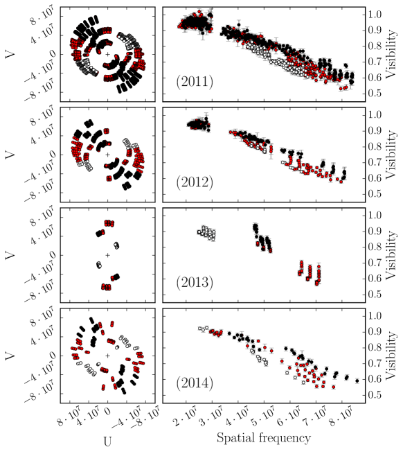
Figure 1: Left: spatial frequencies (u,v) coverage for each dataset. Right: visibility amplitudes (with their respective error bars) as a function of spatial frequency ($B/\lambda$ in units of rad^-1) for each dataset. Epochs 2011, 2012, 2013, and 2014 are represented from top to bottom. Colors indicate position angle (PA) ranges. Black circles correspond to regions around polar axis of the star $PA_{\mathrm{pol}}=36.9^{\circ}$ ($14.4^{\circ}\leq PA\leq 59.4^{\circ}$), hollow circles match the equatorial axis $PA_{\mathrm{eq}}=126.9^{\circ}$ ($104.4^{\circ}\leq PA\leq 159.4^{\circ}$), and red circles correspond to the other directions.

Fig. 1 presents (u,v) coverage and visibility as a function of spatial frequency for each dataset. The slope of the visibility function is different in the polar and equatorial directions owing to the flattening of the photosphere of the star (see Fig. 1). We do not show the closure phases as they are almost all compatible with zero.

The (u,v) coverage for each dataset, except that of 2013, is very uniform, which is a relevant condition for image reconstruction. The angular resolution of the observations is sufficient to reconstruct the global shape of the object and especially resolve any extended structure around the star.

3 Image reconstruction procedure

We used the MiRA software developed by Thiébaut (2008), combined with a Monte Carlo (MC) approach to reconstruct the images for the observations in 2011, 2012, and 2014 because the (u,v) coverage in 2013 is insufficient. The MiRA software is based on an iterative process, starting from an initial image, modifying it to find the pixel values $x_{i}$ which minimize a distance between the interferometric data $d_{i}$ and the same interferometric observables calculated from the image $m_{i}$. This software uses a Bayesian framework and an advanced gradient descent algorithm to find the best solution to this ill-posed problem. The distance between the interferometric data and the image is posed as $\chi^{2}=\sum_{i}\frac{(d_{i}-m_{i})^{2}}{\sigma_{i}^{2}}$, where $\sigma_{i}$ is the data noise. The process of minimizing this distance is conducted under additional constraints of positivity, normalization, and generic constraints on the image, called regularization. The regularization has a global weight relative to the distance between data and image. This weight is usually called hyperparameter and noted as $\mu$. The minimization criterion for the image reconstruction process is then $C=\chi^{2}+\mu\times R$. Finding the right value for $\mu$ is usually difficult, but new ideas using MC methods provide a proxy to this value.

We used a Gaussian prior with varying sizes to concentrate the flux in the central part of the image (see next paragraph). We set the pixel size of the image reconstruction to 0.07 mas. In our case, we used 1000 reconstructed MiRA images of Achernar for both tuning the hyperparameter, with the L-curve method (Kluska et al., 2014) following Dalla Vedova (2016); Domiciano de Souza et al. (2014), and for producing the final image using the Brute-Force Monte Carlo technique (BFMC; see Millour et al., 2012).

The L-curve method is a graph of $\mu$ as a function of the distance to the data $\chi^{2}$. The obtained curve shows a plateau of low $\chi^{2}$ values for lower values of $\mu$, and a steep increase afterward. Selecting the reconstructions among these low $\chi^{2}$ values plateau ensures a good match of the reconstruction to the data, while preserving the benefits of regularization.

The BFMC method works as follows. We reconstructed 1000 images with random values of $\mu$ (in the $[1:1\cdot 10^{9}]$ range), a random start image, and random size of the Gaussian prior, scanning through the parameter space of image reconstruction. We kept the subset of reconstructed images with the smaller distance to the data, in our case $\chi^{2}\leq 2\chi^{2}_{\rm min}$, and the optimum regularization strength evaluated with the L-curve method, in our case $200\leq\mu\leq 300$. We then calculated the average image by calculating the mean of each pixels based on the selected reconstructed images, after centering them. Centering the images is essential to saving the angular resolution of the observations because closure phases do not contain the absolute astrometric position of the star (van Altena, 2012, section 11.7.2) and the individual reconstructed images end up in a random position. The companion star is likely outside the $\approx$200 mas field of view of the observations and does not affect the image reconstruction.

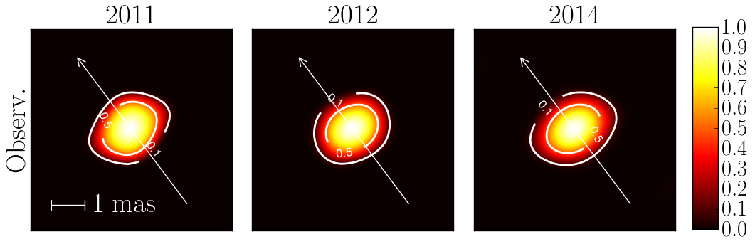
Figure 2: Reconstructed image of Achernar for, from left to right, the 2011, 2012, and 2014 datasets. East is left and north is up. The long arrow shows the previously estimated position angle of the rotation axis of the star on the plane of sky. The dynamic of the images is equal to 1.

The Fig. 2 presents the resulting reconstructed images of Achernar for the 2011, 2012, and 2014 sets of observations. The 2011 and 2012 images show a flattened star similar to previous reconstructions (see Domiciano de Souza et al., 2014), but the 2014 image show extended equatorial emission in addition to the flattened photosphere, which we need to compare with the noise and image reconstruction artefacts level to determine if this is a real structure or not.

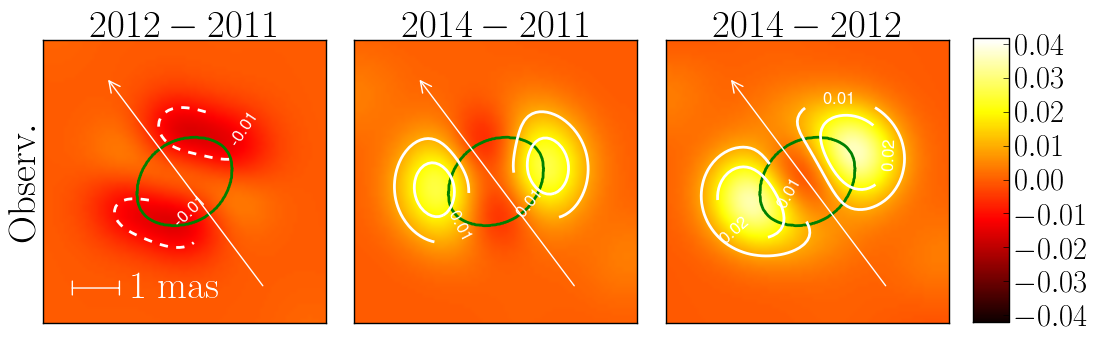
Figure 3: Subtraction of the Achernar reconstructed between different epochs. From left to right, subtraction between the 2012 and 2011 images, subtraction between the 2014 and 2011 images, and subtraction between the 2014 and 2011 images. East is left and north is up. The long arrow shows the previously estimated position angle of the rotation axis of the star on the plane of sky. The green ellipse indicates the delimiting profile of the RvZ model of the photosphere model of Achernar, and the images are highlighted with contours -0.02, -0.01, 0.01, and 0.02.

A way to investigate if this extended equatorial structure is real is to compare the images at different epochs. Fig. 3 shows the subtraction between the reconstructed images of Achernar over the three epochs: 2012-2011, 2014-2011, and 2014-2012. The two subtracted images, including the 2014 observations (2014-2011 and 2014-2012), present an excess of flux of $\sim 4\%$ that is not present in the 2011-2012 subtracted image. This excess can be attributed to a gas disk forming around the main star.

These subtracted images allow us to estimate the size and orientation of the close circumstellar disk independently from any model. From the subtracted images 2014-2011 and 2014-2012, we estimate the equatorial disk diameter in the H band to be between 3.4(4.2) and 3.7(4.5) mas, considering the external limits of the 0.02(0.01) level contours. This corresponds to the angular diameter of the circumstellar region emitting most of the H-band flux. The extreme values of these angular size estimates translates into a disk radius between 1.7 and 2.3 stellar equatorial radii (adopting the equatorial angular diameter of 1.99 mas).

This model-independent size estimate of the H-band emission region is in good agreement with predictions from theoretical models. Indeed, the formation loci of continuum emission at various wavelengths for different Be disk models were computed by Rivinius et al. (2013); Vieira et al. (2015); Carciofi (2011). According to the results of these authors, most ($>80\%$) of the H-band disk flux is emitted within a radius between $\sim 1.5$ to $\sim 4$ times the photospheric equatorial radius, which matches well our estimated disk size.

4 Modeling

We considered two models of Achernar to check if there are indeed variations in the shape of the star between all the considered epochs.

4.1 Roche-von Zeipel model with CHARRON

As a starting point, we adopted the same photospheric model as in Domiciano de Souza et al. (2014). We adopted the Roche approximation (rigid rotation and mass concentrated in the stellar center), which is well adapted for rapidly rotating stars, to model the photosphere of Achernar. We use the code CHARRON (Code for High Angular Resolution of Rotating Objects in Nature) described in detail by Domiciano de Souza et al. (2012a, b, 2002). The star is flattened (equatorial radius larger than the polar radius) because of the important centrifugal force generated by the high rotation velocity of the star. The effective temperature $T_{\mathrm{eff}}$ at the surface depends on the colatitude $\theta$ due to the decreasing effective gravity $g_{\mathrm{eff}}$ (gravitation plus centrifugal acceleration) from the poles to the equator (gravity darkening effect). The resulting map can be seen in the left panel of Fig. 4. This map corresponds to the model parameter values determined by Domiciano de Souza et al. (2014).

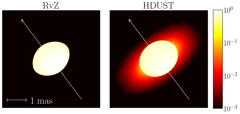
Figure 4: Logarithmic of the normalized intensity maps in the H band for the two models used in this paper. Left: RvZ model computed with the CHARRON code with the model parameter values given by Domiciano de Souza et al. (2014). Right: HDUST model with an ellipsoidal photosphere similar to the RvZ model and a circumstellar viscous decretion disk model (further details in Faes, 2015, Chapter 6). The flux ratio of photosphere and disk model relative to the purely photospheric emission is 1.023.

From this model and the (u,v) coordinates of the observations, we calculated the corresponding synthetic visibilities and computed the residuals between the model and observations at all epochs.

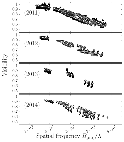
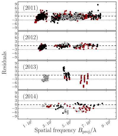
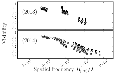
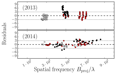
Figure 5: Roche-von Zeipel model compared to the Achernar data. Left: Observed (black dots) and modeled (white stars) visibilities of Achernar. Right: Residual of the visibility between the observations and the RvZ model as a function of the spatial frequency for each dataset. Colors indicate polar and equatorial axes, respectively, as in Fig. 1.

Figure 6: Visibilities of HDUST model compared to the Achernar visibilities. Left: Observed (black dots) and modeled (white stars) visibilities of Achernar. Right: Residual of the visibility between the observations and the HDUST model as a function of the spatial frequency for each dataset. Black and white dots indicate polar and equatorial axes, respectively, such as in Fig. 1.

Fig. 6 shows a comparison of these modeled and observed visibilities along with the computed residuals as a function of the spatial frequencies for each dataset. The model visibilities match the data in 2011 and 2012, but we can see clear departures in 2013 (especially around the frequency $3\times 10^{7}$ rad^-1) and 2014 (especially between $4\times 10^{7}$ rad^-1 and $7\times 10^{7}$ rad^-1).

This is confirmed by the residuals (right panel of Fig. 6), which are contained between the $\pm 3\sigma$ typical limit, with a few outliers in 2011 and 2012, but that clearly diverge above $3\sigma$ in 2013 and 2014, especially in the equatorial direction (hollow dots). This excess residual provides evidence of the presence of an elongated structure around the stellar equator, confirming the excess equatorial emission seen in the reconstructed images.

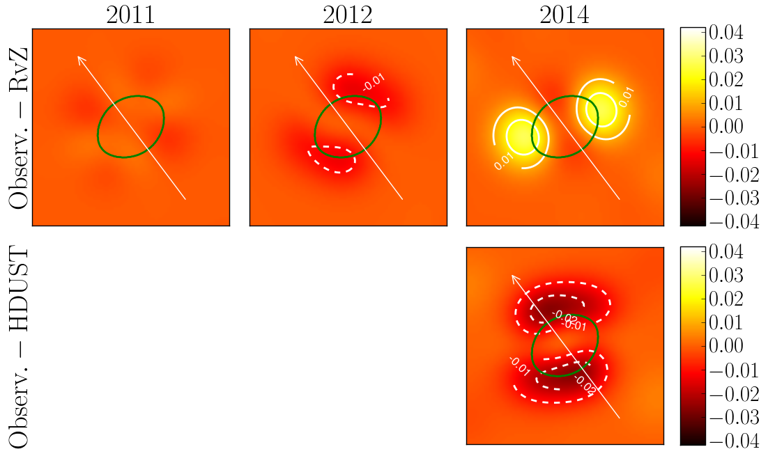
Figure 7: Subtraction between the reconstructed image of Achernar and both the RvZ and HDUST models. On the top row, subtraction between the images reconstructed from the observed data and artificial data calculated from the RvZ model of the photosphere of the star. On the bottom row, subtraction between the reconstructed image from the observed data and from the artificial data calculated form the HDUST model of the photosphere and circumstellar disk. The dynamic of the images is equal to 1. The green ellipse indicates the profile of the RvZ model of the photosphere model of Achernar. The subtraction images are highlighted with contours -0.02, -0.01, 0.01, 0.02. East is left and north is up. The long arrow shows the previously estimated position angle of the rotation axis of the star on the plane of sky. All datasets have been submitted to the same image reconstruction procedure.

4.2 Circumstellar disk model with HDUST

To model this discrepancy between the RvZ model and observed data in 2013 and 2014, we add a circumstellar environment to Achernar by using the 3D, NLTE Monte Carlo radiative transfer code HDUST, which was developed by Carciofi & Bjorkman (2006). We briefly describe HDUST here, while a more detailed description is provided in the above paper. The central star is modeled by an oblate ellipsoid of revolution with identical flattening as the Roche model. Gravity darkening is also included in the model to obtain the surface distribution of effective temperature.

The circumstellar environment is modeled by iterating on the radiative and statistical equilibrium equations to calculate the H-level populations, electron temperatures, and hydrostatic equilibrium density for all grid cells. These calculations include collisional and radiative processes (bound-bound, bound-free, and free-free). In agreement with several recent results on Be star disks, the adopted physical structure and velocity field of the circumstellar disk of Achernar follow the viscous decretion disk (VDD) model (e.g., Rivinius et al., 2013; Carciofi, 2011). Using the oblate photosphere and VDD prescription, Faes (2015, Chapter 6) computed a HDUST disk model that roughly agrees with the polarization and H$\alpha$ spectra of Achernar in 2014. The values for the equatorial radius, flattening, and gravity darkening coefficient adopted for the oblate ellipsoid photospheric model are those from Domiciano de Souza et al. (2014). The resulting intensity map can be seen in Fig. 4, right, and the corresponding H$\alpha$ line profile is given in Fig. 3.

Following our method in Sect. 4.1, we computed visibilities out of this model map and compared them with the observed visibilities in Fig. 6. There is no point in comparing the HDUST model with 2011 and 2012, where the RvZ model neatly matches the data (a comparison that was already carried out in Domiciano de Souza et al., 2014), therefore, Fig. 6 only shows 2013 and 2014. We see a clear improvement of the visual match of visibilities between the RvZ model and HDUST model. This is confirmed by the residual plot, where the residuals shrink within $\pm 3\sigma$, and the computed $\chi^{2}$ values from Table 2 go from 9.7 to 4.8, and 7.9 to 4.4 in 2013 and 2014, respectively.

Table 2: Computed reduced $\chi^{2}$ values for the different models considered in this paper. The reduced $\chi^{2}$ for the HDUST model in 2011 & 2012, with values around 5, is not relevant for this study.

Date	Red. $\chi^{2}$ CHARRON	Red. $\chi^{2}$ HDUST
2011	1.8	-
2012	1.6	-
2013	9.7	4.8
2014	7.9	4.4

The match is not perfect though, mainly because the HDUST model is not actually fitted to the data but just compared with it. Such a fit is beyond the scope of this paper and will be the subject of a forthcoming work (Faes et al., in prep.).

With these two models, one with a naked star and one with a gas disk, we provide the confirmation that our images indeed exhibit a disk very close to the star in 2014, and no disk in 2011 and 2012.

5 Comparison between images and model

For each set of observations, we also reconstructed an image of both the RvZ and HDUST models, as if they had been observed with PIONIER. For that, we produced synthetic data with the same UV coverage and the same error bars as the observations, but with values of visibilities and closure phases replaced by those directly extracted from the RvZ and HDUST models. The same procedure as in Sect. 3 was applied to these synthetic data to get reconstructed images of the model, giving us a common basis for the comparison with the images.

We used a photosphere model that does not include any polar wind nor any companion star, even if both could be present in our data. The polar wind signature may be seen in 2011 and 2012 at the smallest frequencies from the systematic offset seen in the residuals in Fig. 6. However, in the polar direction, we only have long baselines that are less sensitive to an extended polar wind. The companion star signature would produce an increased scatter along all the frequencies, as it is relatively far away from the main star and it contributes to only a few percent of the total H-band flux. Studying these aspects in detail is beyond the scope of this work.

We convolved the final images with a beam of size equal to the effective resolution of the observations, i.e., 1.3 mas. We normalized the dynamic range to 1 and we centered both images before subtracting the image of the model to the image based on the real data. Such a procedure is biased if one wants to compute accurate excess fluxes, but we lack precise H-band photometry inside and outside the line-emission period of Achernar, which would enable us to set the total flux of each component. Therefore, this method provides us only a lower value of the excess flux.

The result is shown in Fig. 7 in which we present the subtraction between the images reconstructed from the observed data and the images reconstructed from the artificial data generated from the RvZ and HDUST models. For the same reason as in Section 4.2, we do not show the subtraction of the HDUST images to the 2011 and 2012 images.

The subtracted images show clearly a variation of the shape of the object during the period from 2011 to 2014. These images show no clear structure around the star in 2011 and 2012, but in 2014 there is an excess of flux on the order of $5\%$ locally that is non-negligible for the instrument sensibility of $\sim 1\%$. Using the HDUST model image improved the situation, confirming that this equatorial excess flux could indeed be explained by the gas disk.

This disk structure is tilted by $18.5^{\circ}\pm 6^{\circ}$ from the equatorial direction of the star. We do not know at this point if this misalignment is significant or not, given the amount of processing we used to retrieve this disk image. This misalignment could be related to disk variability in Achernar, as found by Carciofi et al. (2007). Indeed, blobs of matter are expelled from the photosphere of Achernar and form rings of matter around the star that can be detected by means of rapid polarization angle variations from 30^∘ to 36^∘.

6 Discussion and conclusions

In this paper we have presented H-band images of the Be star Achernar at different epochs corresponding to normal B and Be phases. These images were obtained from image reconstructed techniques applied to VLTI/PIONIER observations taken at three different epochs (2011, 2012, and 2014). While the images do not show any disk (within a $\sim\pm 1\%$ level) in 2011-2012 (see Domiciano de Souza et al., 2014), the image from 2014 data shows that a disk was present mainly around the equatorial region of Achernar. This is in line with the Achernar outburst detected in the beginning of 2013. Follow-up spectroscopic and polarimetric observations showed a growing disk throughout 2013 and 2014 (Faes et al., 2015).

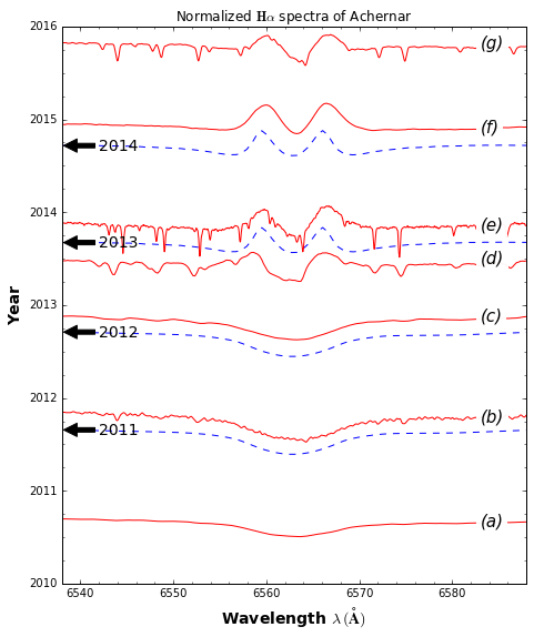
Figure 8: Normalized H$\alpha$ line profiles of Achernar taken at different epochs between the end of 2011 and the end of 2015. The arrows indicate the PIONIER observations corresponding to Table 1. The dashed lines correspond to the model H$\alpha$ line profile computed (1) with CHARRON (see Sect. 4.1) for the photospheric RvZ model (epochs 2011 and 2012) and (2) with HDUST (see Sect. 4.2) for the photosphere and disk model (epochs 2013 and 2014).

Fig. 3 shows several of these H$\alpha$ spectra of Achernar taken at different epochs covering the PIONIER observations. Details of each spectrum are given in the caption of the figure. H$\alpha$ is in absorption before end of 2012, so that the 2011 and 2012 PIONIER data were recorded when Achernar was essentially in a normal B phase (a thorough discussion on this phase pre-2013 is given by Domiciano de Souza et al., 2014). On the other hand, as shown in Fig. 3, H$\alpha$ is in clear emission from mid-2013 to at least the end of 2015, meaning that the 2013 and 2014 PIONIER data were recorded with Achernar in an emission-line phase (Be phase).

From the 2014 reconstructed image compared to the 2011 and 2012 images, we estimated that the near-IR contribution of the disk extends to $\sim 1.7-2.3$ equatorial radii, independently from any modeling. This result is in good agreement with predictions from theoretical Be-disk models, providing direct support to them.

Although the question of the physical mechanism triggering the ejection of material from the star followed by disk formation is still unanswered, the results from this work provide direct information about the near-IR size and flux of a newly formed Be disk, which will contribute to future works on the disk formation and dissipation processes in Be stars and massive stars in general.