Reaction-Diffusion Systems in Epidemiology

Abstract

A key problem in modelling the evolution dynamics of infectious diseases is the mathematical representation of the mechanism of transmission of the contagion which depends upon the way the specific disease is communicated among different populations or subpopulations. Compartmental models describing a finite number of subpopulations can be described mathematically via systems of ordinary differential equations. The same is not possible for populations which exhibit some continuous structure, such as space location, age, etc. In particular when dealing with populations with space structure the relevant quantities are spatial densities, whose evolution in time requires now nonlinear partial differential equations, which are known as reaction-diffusion systems. In this chapter we are presenting an (historical) outline of mathematical epidemiology, paying particular attention to the role of spatial heterogeneity and dispersal in the population dynamics of infectious diseases. Two specific examples are discussed, which have been the subject of intensive research by the authors of the present chapter, i.e. man-environment-man epidemics, and malaria. In addition to the epidemiological relevance of these epidemics all over the world, their treatment requires a large amount of different sophisticate mathematical methods, and has even posed new non trivial mathematical problems, as one can realize from the list of references. One of the most relevant problems faced by the present authors, i.e. regional control, has been emphasized here: the public health concern consists of eradicating the disease in the relevant population, as fast as possible. On the other hand, very often the entire domain of interest for the epidemic, is either unknown, or difficult to manage for an affordable implementation of suitable environmental sanitation programmes. This is the reason why regional control has been proposed; it might be sufficient to implement such programmes only in a given subregion conveniently chosen so to lead to an effective (exponentially fast) eradication of the epidemic in the whole habitat; it is evident that this practice may have an enormous importance in real cases with respect to both financial and practical affordability.

KEYWORDS: Epidemic systems; reaction-diffusion systems; man-environment epidemics; malaria; stabilization.

1 Introduction

Apart from D. Bernoulli (1760) [18], those who established the roots of this field of research (in chronological order) were: W. Farr (1840) [48], W.H. Hamer (1906) [51], J. Brownlee (1911) [19], R. Ross (1911) [70], E. Martini (1921) [64], A. J. Lotka (1923) [61], W.O. Kermack and A. G. McKendrick (1927) [56], H. E. Soper (1929) [78], L. J. Reed and W. H. Frost (1930) [50], [1], M. Puma (1939) [69], E. B. Wilson and J. Worcester (1945) [80], M. S. Bartlett (1949) [17], G. MacDonald (1950) [62], N.T.J. Bailey (1950) [16], before many others; the pioneer work by En’ko (1989) [47] suffered from being written in Russian; historical accounts of epidemic theory can be found in [72], [43], [44]. After the late ${}^{\prime}70$’s there has been an explosion of interest in mathematical epidemiology, also thanks to the establishment of a number of new journals dedicated to mathematical biology.

The scheme of this presentation is the following: in Section 1.1 a general structure of mathematical models for epidemic systems is presented in the form of compartmental systems; in Section 1.2 the concept of field of forces of infection is discussed for structured populations.

1.1 Compartmental models

Model reduction for epidemic systems is obtained via the so-called compartmental models. In a compartmental model the total population (relevant to the epidemic process) is divided into a number (usually small) of discrete categories: susceptibles, infected but not yet infective (latent), infective, recovered and immune, without distinguishing different degrees of intensity of infection; possible structures in the relevant population can be superimposed when required (see e.g. Figure 1).

Figure 1: The transfer diagram for an SEIR compartmental model including the susceptible class S, the exposed, but not yet infective, class E, the infective class I, and the removed class R

A key problem in modelling the evolution dynamics of infectious diseases is the mathematical representation of the mechanism of transmission of the contagion which depends upon the way the specific disease is communicated among different populations or subpopulations. This problem has been raised since the very first models when age and/or space dependence had to be taken into account.

Suppose at first that the population in each compartment does not exhibit any structure (space location, age, etc.). Let us ignore, for the time being, the intermediate state $E.$ The infection process ($S$ to $I$) is driven by a force of infection ($f.i.$) due to the pathogen material produced by the infective population and available at time $t$

$$(f.i.)(t)=[g(I(.))](t)$$

which acts upon each individual in the susceptible class. Thus a typical rate of the infection process is given by the

$$(\textnormal{incidence rate})(t)=(f.i.)(t)S(t).$$

From this point of view, the so called “law of mass action” simply corresponds to choosing a linear dependence of $g(I)$ upon $I$

$$(f.i.)(t)=kI(t).$$

The great advantage, from a mathematical point of view, is that the evolution of the epidemic is described (in the space and time homogeneous cases) by systems of ODE ’s which contain at most bilinear terms.

Referring to the “law of mass action”, Wilson and Worcester [80] stated the following:

“It would in fact be remarkable, in a situation so complex as that of the passage of an epidemic over a community, if any simple law adequately represented the phenomenon in detail … even to assume that the new case rate should be set equal to any function … might be questioned”.

Indeed Wilson and Worcester [80], and Severo [73] had been among the first epidemic modelers including nonlinear forces of infection of the form

$$(f.i.)(t)=\kappa I(t)^{p}S(t)^{q}$$

in their investigations. Here $I(t)$ denotes the number of persons who are infective, and $S(t)$ denotes the number of persons who are susceptible to the infection.

Independently, during the analysis of data regarding the spread of a cholera epidemic in Southern Italy during 1973, in [30] one of the authors (V.C.) suggested the need to introduce a nonlinear force of infection in order to explain the specific behavior emerging from the available data.

A more extended analysis for a variety of proposed generalizations of the classical models known as Kermack-McKendrick models, appeared in [31], though nonlinear models became widely accepted in the literature only a decade later, after the paper [60].

Nowadays models with nonlinear forces of infection are analyzed within the study of various kinds of diseases; typical expressions include the so called Holling type functional responses (see e.g. [31], [53])

$$(f.i.)(t)=g(I(t))\,\,\,;$$

with

$$g(I)=\displaystyle{{k\,\,I^{p}}\over{\alpha+\beta\,\,\displaystyle{I^{q}}}}\,\,\,\,,\qquad p,q\,\,>0\,\,\,.$$ (1.1)

Particular cases are

$$g(I)=k\,\,I^{p}\,\,\,\,,\qquad p>0$$ (1.2)

For the case $p=q$ we have the behaviors described in Figure 2.

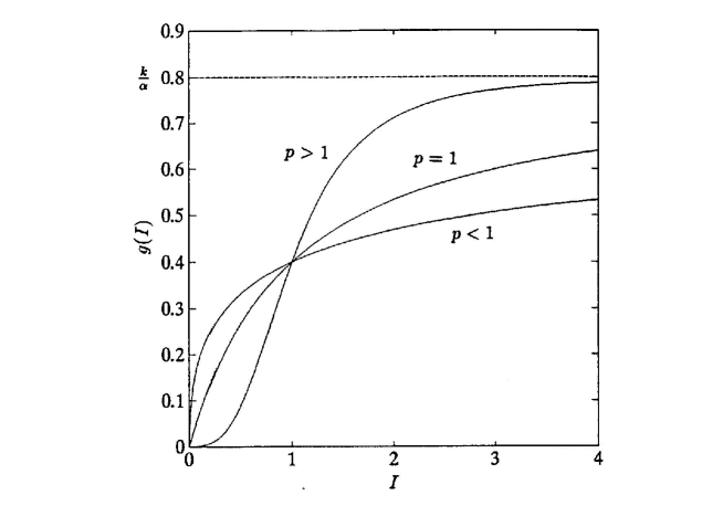
Figure 2: Nonlinear forces of infection [31]

Additional shapes of $g(I),$ as proposed in [31] which may decrease for large values of $I,$ may be interpreted as “awareness” effects in the contact rates. Significant contributions to this concept and related epidemiological issues in recent literature can be found in [46].

Further extensions include a nonlinear dependence upon both $I$ and $S$, as discussed in modelling AIDS epidemics (see e.g. [34], [35], and references therein), where the social structure of the host population is analyzed too.

1.2 Structured populations

Compartmental models with a finite number of compartments can be described mathematically via systems of ordinary differential equations (ODE’s). The same is not possible for populations which exhibit some continuous structure (identified here by a parameter $z$), such as space location, age, etc.

When dealing with populations with space structure the relevant quantities are spatial densities, such as $s(z;t)$ and $i(z;t)$, the spatial densities of susceptibles and of infectives respectively, at a point $z$ of the habitat $\Omega$, and at time $t\geq 0,$ such that the corresponding total populations are given by

$$S(t)=\int_{\Omega}{s(z;t)\,\,dz},\qquad I(t)=\int_{\Omega}{i(z;t)\,\,dz}$$

The role of spatial heterogeneity and dispersal in population dynamics has been the subject of much research. We shall refer here to the fundamental literature on the subject by quoting [8], [13], [49], [55], [58], [66], [68], [74], [76].

In the theory of propagation of infectious diseases the motivation of the study of the effects of spatial diffusion is mainly due to the large scale impact of an epidemic phenomenon; this is discussed in detail in [39].

We will choose here as a good starting point the pioneer work by D.G. Kendall who modified the basic Kermack-McKendrick SIR model to include the effects of spatial heterogeneity in an epidemic system [55].

Kendall ’s work has motivated a lot of research in the theory of epidemics with spatial diffusion. In particular two classes of problems arise according to the size of the spatial domain or habitat.

If the habitat is unbounded, travelling waves are of interest [55], [54], [11], [41], [79]. A nice introduction to the subject can be found in [66].

If, on the other hand, the habitat is a bounded spatial domain then problems of existence of nontrivial endemic states (possibly with spatial patterns) are of interest [21].

Usually reaction diffusion systems (see e.g. [49]) are seen as an extension of compartmental systems in which each compartment, representing a different species, is allowed to invade a spatial domain $\,\Omega\subset\mathbb{R}^{m}\,$ with a space dependent density. Densities interact among themselves according to the same mathematical laws which were used for the space independent case, but are subject individually to a spatial diffusion mechanism usually committed to the Laplace operator, which simulates random walk or Brownian motion of the interacting species [12], [49].

Typically then a system of $\,n\,$ interacting species, each of them having a spatial density

$$\left\{u_{i}(x;t),\quad x\in\Omega\right\},\quad i=1,\ldots,n\quad\hbox{\rm at time}\quad t\geq 0,$$

is described by the following system of semilinear parabolic equations:

$${\frac{\partial u}{\partial t}=D\Delta u(x;t)+f(u(x;t))}$$ (1.3)

in $\Omega\times\mathbb{R}_{+},$ subject to suitable boundary conditions.

Here $\,u=(u_{1},\ldots,u_{n})^{T}\,;\,\,\,D=diag(d_{1},\ldots,d_{n}),\,\,\,\hbox{\rm and}\,\,\,f(z)\,,\,\,\,z\in\mathbb{R}^{n}\,$ is the interaction law among the species via their densities.

A derivation and discussion of Equation (1.3) can be found in [49] (see also [68]).

In Equation (1.3) $\,f(z)\,,\,\,\,z\in\mathbb{R}^{n},$ usually is the same interaction function of the classical compartmental approach. Thus for an SIR model (including Susceptible, Infective, and Removed individuals) with vital dynamics, Equation (1.3) is written as follows

$$\left\{\begin{array}[]{ll}\displaystyle{\frac{\partial s}{\partial t}(x;t)=d_{1}\Delta s(x;t)-k\,i(x;t)\,s(x;t)+\mu-\mu\,s(x;t)}\\ \vskip 3.0pt plus 1.0pt minus 1.0pt\\ \displaystyle{\frac{\partial i}{\partial t}(x;t)=d_{2}\Delta i(x;t)+k\,i(x;t)\,s(x;t)-(\mu+\gamma)\,i(x;t)}\\ \vskip 3.0pt plus 1.0pt minus 1.0pt\\ \displaystyle{\frac{\partial r}{\partial t}(x;t)=d_{3}\Delta r(x;t)+\gamma\,i(x;t)-\mu\,r(x;t)}\end{array}\right.$$ (1.4)

where now $\,s(x;t)\,,\,\,i(x;t)\,,\,\,r(x;t)\,$ are the corresponding spatial densities of $S,I,R$:

$$S(t)=\int_{\Omega}s(x;t)\,dx;\quad I(t)=\int_{\Omega}i(x;t)\,dx;\quad R(t)=\int_{\Omega}r(x;t)\,dx.$$

Thus the infection process is represented by a   “local” interaction of two densities $s(x;t)$ and $i(x;t),$ at point $x\in\Omega$ and time $t\in\mathbb{R}_{+},$ via the following “law of mass action”

$$(f.i.)(z;t)=k\,i(x;t)\,s(x;t)$$ (1.5)

In Kendall ’s model [55] (1.5) is substituted by an “integral” interaction between the infectives and the susceptibles; the force of infection acting at point $x\in\Omega$ and time $t\in\mathbb{R}_{+}$ is given by

$$g(i(\cdot;t))(x)=\int_{\Omega}k(x,x^{\prime})\,i(x^{\prime};t)\,dx^{\prime},$$ (1.6)

where $k(x,x^{\prime})$ describes the influence, by any reason, of the infectives located at any point $x^{\prime}\in\Omega$ on the susceptibles located at point $x\in\Omega$.

As a consequence the infection process is described now by

$$(f.i.)(z;t)=g(i(\cdot;t))(x)\,s(x;t).$$ (1.7)

Clearly we reobtain (1.5) in the limiting case $\,k(x,x^{\prime})=\delta(x-x^{\prime})\,$ (the Dirac function).

As one can see, (1.7) better fits the philosophy introduced in Section 1 to allow $g(I)$, the force of infection due to the population of infectives, and acting on the susceptible population, to have a general form which case by case takes into account the possible mechanisms of transmission of the disease.

For Problem (1.4) we refer to the literature [11], [21], [41], [79]. For the case in (1.6)-(1.7) the emergence of travelling waves has been shown in [55] and [11]. The analysis of the diffusion approximation of Kendall’s model can be found in [54].

When dealing with populations with an age structure, we may interpret the parameter $z$ as the age-parameter so that the first model above is a model with intracohort interactions while the second one is a model with intercohort interactions (see e.g. [20], and references therein).

A large literature on the subject can be found in [23].

2 Specific examples

2.1 Spatially structured man-environment-man epidemics

A widely accepted model for the spatial spread of epidemics in an habitat $\Omega$, via the environmental pollution produced by the infective population, e.g. via the excretion of pathogens in the environment, is the following one, as proposed in [21], [22] (see also [23], and references therein). The model below is a more realistic generalization of a previous model proposed by one of the authors (V. C.) and his co-workers [27], [25], [30] to describe fecal-orally transmitted diseases (cholera, typhoid fever, infectious hepatitis, etc.) which are typical for the European Mediterranean regions; it can anyhow be applied to other infections, and other regions, which are propagated by similar mechanisms (see e.g. [40]); schistosomiasis in Africa is a typical additional example [67].

$$\left\{\begin{array}[]{ll}\displaystyle{{\partial u_{1}}\over{\partial t}}(x,t)=d_{1}\Delta u_{1}(x,t)\displaystyle-a_{11}u_{1}(x,t)+\int_{\Omega}k(x,x^{\prime})u_{2}(x^{\prime},t)dx^{\prime}\vspace{2mm}\\ \displaystyle{{\partial u_{2}}\over{\partial t}}(x,t)=-a_{22}u_{2}(x,t)+g(u_{1}(x,t))\end{array}\right.$$ (2.1)

in $\Omega\subset{\bf R}^{N}\,\ (N\geq 1)$, a nonempty bounded domain with a smooth boundary $\partial\Omega$; for $t\in(0,+\infty)$, where $a_{11}\geq 0$, $a_{22}\geq 0,~{}d_{1}>0$ are constants.

• $u_{1}(x,t)$ denotes the concentration of the pollutant (pathogen material) at a spatial location $x\in\overline{\Omega},$ and a time $t\geq 0;$

• $u_{2}(x,t)$ denotes the spatial distribution of the infective population.

• The terms $-a_{11}u_{1}(x,t)$ and $-a_{22}u_{2}(x,t)$ model natural decays.

• The total susceptible population is assumed to be sufficiently large with respect to the infective population, so that it can be taken as constant.

For this kind of epidemics the infectious agent is multiplied by the infective human population and then sent to the sea through the sewage; because of the peculiar eating habits of the population of these regions the agent may return via some diffusion-transport mechanism to any point of the habitat $\Omega,$ where the infection process is further activated; thus the integral term

$$\int_{\Omega}k(x,x^{\prime})u_{2}(x^{\prime},t)dx^{\prime}$$

expresses the fact that the pollution produced at any point $x^{\prime}\in\Omega$ of the habitat is made available at any other point $x\in\Omega$; when dealing with human pollution, this may be due to either malfunctioning of the sewage system, or improper dispersal of sewage in the habitat. Linearity of the above integral operator is just a simplifying option.

The Laplace operator takes into account a simplified random dispersal of the infectious agent in the habitat $\Omega,$ due to uncontrolled additional causes of dispersion (with a constant diffusion coefficient to avoid purely technical complications); we assume that the infective population does not diffuse (the case with diffusion would be here a technical simplification). As such, System (2.1) can be adopted as a good model for the spatial propagation of an infection in agriculture and forests, too.

Finally, the local “incidence rate” at point $x\in\Omega,$ and time $t\geq 0$, is given by

$$(i.r.)(x,t)=g(u_{1}(x,t)),$$

depending upon the local concentration of the pollutant.

The parameters $a_{11}$ and $a_{22}$ are intrinsic decay parameters of the two populations.

2.2 Seasonality.

If we wish to model a large class of fecal-oral transmitted infectious diseases, such as typhoid fever, infectious hepatitis, cholera, etc., we may include the possible seasonal variability of the environmental conditions, and their impact on the habits of the susceptible population, so that the relevant parameters are assumed periodic in time, all with the same period $T\in(0,+\infty)$.

As a purely technical simplification, we may assume that only the incidence rate is periodic, and in particular that it can be expressed as

$$(i.r.)(x,t)=h(t,u_{1}(x,t))=p(t)g(u_{1}(x,t)),$$

where $h$, the functional dependence of the incidence rate upon the concentration of the pollutant, can be chosen as in the time homogeneous case, with possible behaviors as shown in Figure 2.

The explicit time dependence of the incidence rate is given via the function $p(\cdot),$ which is assumed to be a strictly positive, continuous and $T-$periodic function of time; i.e. for any $t\in\mathbb{R},$

$$p(t)=p(t+T).$$

Remark 1. The results can be easily extended to the case in which also $a_{11}$, $a_{22}$ and $k$ are $T-$periodic functions.

In [22] the above model was studied, and sufficient conditions were given for either the asymptotic extinction of an epidemic outbreak, or the existence and stability of an endemic state; while in [29] the periodic case was additionally studied, and sufficient conditions were given for either the asymptotic extinction of an epidemic outbreak, or the existence and stability of a periodic endemic state with the same period of the parameters.

2.3 Saddle point behaviour.

The choice of $g$ has a strong influence on the dynamical behavior of system (2.1). The case in which $g$ is a monotone increasing function with constant concavity has been analyzed in an extensive way (see [23], [26], [28]); concavity leads to the existence (above a parameter threshold) of exactly one nontrivial endemic state and to its global asymptotic stability. In order to better clarify the situation, consider first the spatially homogeneous case (ODE system) associated with system (2.1); namely

$$\left\{\begin{array}[]{ll}\displaystyle{{dz_{1}}\over{dt}}(t)=\displaystyle-a_{11}z_{1}(t)+a_{12}z_{2}(t)\vspace{2mm}\\ \displaystyle{{du_{2}}\over{dt}}(t)=-a_{22}z_{2}(t)+g(z_{1}(t))\end{array}\right.$$ (2.2)

In [28] and [67] the bistable case (in which system (2.2) may admit two nontrivial steady states, one of which is a saddle point in the phase plane) was obtained by assuming that the force of infection, as a function of the concentration of the pollutant, is sigma shaped. In [67] this shape had been obtained as a consequence of the sexual reproductive behavior of the schistosomes. In [28] (see also [27]) the case of fecal-oral transmitted diseases was considered; an interpretation of the sigma shape of the force of infection was proposed to model the response of the immune system to environmental pollution: the probability of infection is negligible at low concentrations of the pollutant, but increases with larger concentrations; it then becomes concave and saturates to some finite level as the concentration of pollutant increases without limit.

Let us now refer to the following simplified form of System (2.1), where as kernel we have taken $k(x,x^{\prime})=a_{12}\delta(x-x^{\prime}),$

$$\left\{\begin{array}[]{ll}\displaystyle{{\partial u_{1}}\over{\partial t}}(x,t)=d_{1}\Delta u_{1}(x,t)\displaystyle-a_{11}u_{1}(x,t)+a_{12}u_{2}(x,t)\vspace{2mm}\\ \displaystyle{{\partial u_{2}}\over{\partial t}}(x,t)=-a_{22}u_{2}(x,t)+g(u_{1}(x,t))\end{array}\right.$$ (2.3)

The concavity of $g$ induces concavity of its evolution operator, which, together with the monotonicity induced by the quasi monotonicity of the reaction terms in (2.3), again imposes uniqueness of the possible nontrivial endemic state. On the other hand, in the case where $g$ is sigma shaped, monotonicity of the solution operator is preserved, but as we have already observed in the ODE case, uniqueness of nontrivial steady states is no longer guaranteed. Furthermore, the saddle point structure of the phase space cannot be easily transferred from the ODE to the PDE case, as discussed in [28], [33]. In [28], homogeneous Neumann boundary conditions were analyzed; in this case nontrivial spatially homogeneous steady states are still possible. But when we deal with homogeneous Dirichlet boundary conditions or general third-type boundary conditions, nontrivial spatially homogeneous steady states are no longer allowed. In [33] this problem was faced in more detail; the steady-state analysis was carried out and the bifurcation pattern of nontrivial solutions to system (2.3) was determined when subject to homogeneous Dirichlet boundary conditions. When the diffusivity of the pollutant is small, the existence of a narrow bell-shaped steady state was shown, representing very likely a saddle point for the dynamics of (2.3). Numerical experiments confirm the bistable situation: “small” outbreaks stay localized under this bell-shaped steady state, while “large” epidemics tend to invade the whole habitat.

2.4 Boundary feedback

An interesting problem concerns the case of boundary feedback of the pollutant, which has been proposed in [26], and further analyzed in [32]; an optimal control problem has been later analyzed in [9].

In this case the reservoir of the pollutant generated by the human population is spatially separated from the habitat by a boundary through which the positive feedback occurs. A model of this kind has been proposed as an extension of the ODE model for fecal-oral transmitted infections in Mediterranean coastal regions presented in [30].

For this kind of epidemics the infectious agent is multiplied by the infective human population and then sent to the sea through the sewage system; because of the peculiar eating habits of the population of these regions, the agent may return via some diffusion-transport mechanism to any point of the habitat, where the infection process is restarted.

The mathematical model is based on the following system of evolution equations:

$$\left\{\begin{array}[]{ll}\displaystyle{\frac{\partial u_{1}}{\partial t}}(x;t)=\Delta u_{1}(x;t)-a_{11}u_{1}(x;t)\\ {}{}{}\\ \displaystyle{\frac{\partial u_{2}}{\partial t}}(x;t)=-a_{22}u_{2}(x;t)+g(u_{1}(x;t))\end{array}\right.$$

in $\Omega\times(0,+\infty)$, subject to the following boundary condition

$${{\partial u_{1}}\over{\partial\nu}}(x;t)+\alpha u_{1}(x;t)=\int_{\Omega}k(x,x^{\prime})u_{2}(x^{\prime};t)\,dx^{\prime}$$

on $\partial\Omega\times(0,+\infty)$, and also subject to suitable initial conditions.

Here $\Delta$ is the usual Laplace operator modelling the random dispersal of the infectious agent in the habitat; the human infective population is supposed not to diffuse. As usual $a_{11}$ and $a_{22}$ are positive constants. In the boundary condition the left hand side is the general boundary operator $B:=\displaystyle{{\partial\over{\partial\nu}}+\alpha(\cdot)}$ associated with the Laplace operator; on the right hand side the integral operator

$$H\left[u_{2}(\cdot,t)\right](x):=\int_{\Omega}k(x,x^{\prime})u_{2}(x^{\prime};t)\,dx^{\prime}$$

describes boundary feedback mechanisms, according to which the infectious agent produced by the human infective population at time $t>0$, at any point $x^{\prime}\in\Omega$, is available, via the transfer kernel $k(x,x^{\prime})$, at a point $x\in\partial\Omega$.

Clearly the boundary $\partial\Omega$ of the habitat $\Omega$ can be divided into two disjoint parts: the sea shore $\Gamma_{1}$ through which the feedback mechanism may occur, and $\Gamma_{2}$ the boundary on the land, at which we may assume complete isolation.

The parameter $\alpha(x)$ denotes the rate at which the infectious agent is wasted away from the habitat into the sea along the sea shore. Thus one may well assume that

$$\alpha(x),\quad k(x,\cdot)=0,\qquad\hbox{\rm for}\,\,\,\,x\in\Gamma_{2}\,\,\,.$$

A relevant assumption, of great importance in the control problems that we have been facing later, is that the habitat $\Omega$ is ”epidemiologically” connected to its boundary by requesting that

$$\hbox{\rm for any}\,\,\,\,\,x^{\prime}\in\Omega\,\,\,\,\,\hbox{\rm there exists some}\,\,\,\,\,x\in\Gamma_{1}\,\,\,\,\,\hbox{\rm such that}\quad k(x,x^{\prime})>0.$$

This means that from any point of the habitat infective individuals contribute to polluting at least some point on the boundary (the sea shore).

In the above model delays had been neglected and the feedback process had been considered to be linear; various extensions have been considered in subsequent literature.

2.5 Malaria

Malaria is found throughout the tropical and subtropical regions of the world and causes more than 300 million acute illnesses and at least one million deaths annually [81], especially in Africa. Human malaria is caused by one or a combination of four species of plasmodia: Plasmodium falciparum, P. vivax, P. malariae, and P. ovale. The parasites are transmitted through the bite of infected female mosquitoes of the genus Anopheles. Mosquitoes can become infected by feeding on the blood of infected people, and the parasites then undergo another phase of reproduction in the infected mosquitoes.

The earliest attempt to provide a quantitative understanding of the dynamics of malaria transmission was that of Ross [70]. Ross’ models consisted of a few differential equations to describe changes in densities of susceptible and infected people, and susceptible and infected mosquitoes. Macdonald [63] extended Ross’ basic model, analyzed several factors contributing to malaria transmission, and concluded that “the least influence is the size of the mosquito population, upon which the traditional attack has always been made”.

The work of Macdonald had a very beneficial impact on the collection, analysis, and interpretation of epidemic data on malaria infection [65] and guided the enormous global malaria-eradication campaign of his era.

The classical Ross-Macdonald model is highly simplified. Subsequent contributions have been made to extend the Ross-Macdonald malaria models considering a variety of epidemiological features of malaria [10], [42] (see also [15], [37], [38], [45], [57], [71], [75]).

Here we will consider an oversimplified model, concentrating on a problem of possible eradication of a spatially structured malaria epidemic, by acting on the segregation of the human and the mosquito populations via e.g. treated bednets (see e.g. [77]).

Following recent papers by Ruan et al [71], and Chamchod and Britton [36], we divide the human population into two classes, susceptible and infectious, whereas the mosquito population is divided into three classes, susceptible, infectious, and removed because of death. Suppose that the infection in the human does not result death or isolation. For the transmission of the pathogen, it is assumed that a susceptible human can receive the infection only by contacting with infective mosquitos, and a susceptible mosquito can receive the infection only from the infectious human.

For simplicity, assume the total populations of both humans and mosquitoes are constants and denoted by $H$ and $M$, respectively. Let $X(t)$ and $Y(t)$ denote the numbers of infected humans and mosquitoes at time $t$, respectively. Let $a$ be the rate of biting on humans by a single mosquito (number of bites per unit time). Then the number of bites on humans per unit time per human is $\displaystyle{\frac{a}{H}}$. If $b$ is the proportion of infected bites on humans that produce an infection, the interaction between the infected mosquitoes $Y(t)$ and the uninfected humans $H-X(t)$ will produce new infected humans at a rate of of $\displaystyle{\frac{a}{H}}b(H-X(t))Y(t).$ Malaria on humans is an SIS system for which human infectives after recovery go back in the susceptible state; we will denote by $r$ the per capita rate of recovery in humans so that $1/r$ is the duration of the disease in humans [23].

Therefore, the equation for the rate of change in the number of infected humans is

$$\frac{dX}{dt}=-rX(t)+\frac{a}{H}b(H-X(t))Y(t).$$

Similarly, if $\mu$ is the per capita rate of mortality in mosquitoes, so that $1/\mu$ is the life expectancy of mosquitoes, and $c$ is the transmission efficiency from humans to mosquito, then we have the equation for the rate of change in the number of infected mosquitoes:

$$\frac{dY}{dt}=-\mu Y(t)+\frac{a}{H}cX(t)(M-Y(t)).$$

Here we wish to consider a spatially structured system, so that we will refer to spatial densities of infected humans and infected mosquitoes. Specifically, let $u_{1}(x,t)$ denote the spatial density of the population of infected mosquitoes at a spatial location $x\in\overline{\Omega}$ and a time $t\geq 0;$ while $u_{2}(x,t)$ denotes the spatial distribution of the human infective population. In accordance with the above, the spatial density $C(x)$ of the total human population will be assumed constant in time, so that $C(x)-u_{2}(x,t)$ will provide the spatial distribution of susceptible humans, at a spatial location $x\in\overline{\Omega}$ and a time $t\geq 0.$

Hence the “local incidence” for humans, at point $x\in\overline{\Omega}$, and time $t\geq 0$, is taken of the form

$$(i.r.)_{H}(x,t)=g(u_{1}(x,t),u_{2}(x,t))=(C(x)-u_{2}(x,t))h(u_{1}(x,t)),$$

depending upon the local densities of both populations via a suitable functional response $h$.

As pointed out in [65], seasonality of the aggressivity to humans by the mosquito population might also be considered in the functional response $h;$ this has been a topic of the authors research programme in [29], and [5], [4].

As proposed in [15], we will include spatial diffusion of the infective mosquito population (with constant diffusion coefficient to avoid purely technical complications), but we assume that the human population does not diffuse.

On the other hand, inspired by previous models for spatially structured man-environment epidemics (see e.g. [22]), we will modify the infection term of mosquitoes $\displaystyle{\frac{a}{H}}cX(t)(M-Y(t))$ as follows.

Given a habitat $\Omega\subset\mathbf{R}^{N}\,\ (N\geq 2)$ (which is a nonempty bounded domain with a smooth boundary $\partial\Omega$), we assume that the total susceptible mosquito population is so large that it can be considered time and space independent; further we consider the fact that the infected mosquitoes at a location $x\in{\Omega}$ and a time $t\geq 0$ is due to contagious bites to human infectives at any point $x^{\prime}\in\Omega$ of the habitat, within a spatial neighborhood of $x$ represented by a suitable probability kernel $k(x^{\prime},x),$ depending on the specific structure of the local ecosystem; as a trivial simplification one may assume $k(\cdot,x)$ as a Gaussian density centered at $x;$ hence the “local incidence” for mosquitoes, at point $x\in{\ \Omega}$, and time $t\geq 0$, is taken as

$$(i.r.)_{M}(x,t)=\int_{\Omega}k(x,x^{\prime})u_{2}(x^{\prime},t)dx^{\prime}$$

Finally, from now on, we will denote by $-a_{11}u_{1}(x,t)$ the natural decay of the infected mosquito population, while $-a_{22}u_{2}(x,t)$ will denote the recovery rate (back to susceptibility) of the human infective population.

All the above leads to the following over simplified model for the spatial spread of malaria epidemics, in which we have ignored the possible acquired immunity of humans after exposure to the contagion, the possible differentiation of the mosquito population, etc. (see e.g. [57]).

$$\left\{\begin{array}[]{ll}\displaystyle{{\partial u_{1}}\over{\partial t}}(x,t)=d_{1}\Delta u_{1}(x,t)\displaystyle-a_{11}u_{1}(x,t)+\int_{\Omega}k(x,x^{\prime})u_{2}(x^{\prime},t)dx^{\prime}\vspace{2mm}&\\ {{\partial u_{2}}\over{\partial t}}(x,t)=-a_{22}u_{2}(x,t)+g(u_{1}(x,t),u_{2}(x,t))&\end{array}\right.$$

in $\Omega\times(0,+\infty)$, where $a_{11}>0$, $a_{22}>0,~{}d_{1}>0$ are constant.

3 Regional Control: Think Globally, Act Locally

Let us now go back to System (2.1) in $\Omega\subset{\bf R}^{N}\,\ (N\geq 1)$, a nonempty bounded domain with a smooth boundary $\partial\Omega$; for $t\in(0,+\infty)$, where $a_{11}\geq 0$, $a_{22}\geq 0,~{}d_{1}>0$ are constants.

The public health concern consists of providing methods for the eradication of the disease in the relevant population, as fast as possible. On the other hand, very often the entire domain $\Omega,$ of interest for the epidemic, is either unknown, or difficult to manage for an affordable implementation of suitable environmental sanitation programmes. Think of malaria, schistosomiasis, and alike, in Africa, Asia, etc.

This has led the second author, in a discussion with Jacques Louis Lions in 1989, to suggest that it might be sufficient to implement such programmes only in a given subregion $\omega\subset\Omega,$ conveniently chosen so to lead to an effective (exponentially fast) eradication of the epidemic in the whole habitat $\Omega.$ Though, a satisfactory mathematical treatment of this issue has been obtained only few years later in [2]. This practice may have an enormous importance in real cases with respect to both financial and practical affordability. Further, since we propose to act on the elimination of the pollution only, this practice means an additional nontrivial social benefit on the human population, since it would not be limited in his social and alimentation habits.

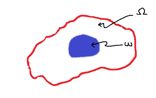
Figure 3: Think Globally, Act Locally.

In this section a review is presented of some results obtained by the authors, during 2002-2012, concerning stabilization (for both the time homogeneous case and the periodic case). Conditions have been provided for the exponential decay of the epidemic in the whole habitat $\Omega,$ based on the elimination of the pollutant in a subregion $\omega\subset\Omega$. The case of homogeneous third type boundary conditions has been considered, including the homogeneous Neumann boundary conditions (to mean complete isolation of the habitat):

$$\frac{\partial u_{1}}{\partial\nu}(x,t)+\alpha u_{1}(x,t)=0\qquad\mbox{\rm on }\partial{\Omega}\times(0,+\infty),$$

where $\alpha\geq 0$ is a constant.

For the time homogeneous case the following assumptions have been taken:

• $\,\,g:\mathbb{R}\rightarrow[0,+\infty)$ is a function satisfying

  • $g(x)=0$,  for $x\in(-\infty,0]$,

  • $g$ is Lipschitz continuous and increasing,

  • $g(x)\leq a_{21}x,\ \mbox{\rm for any }x\in[0,+\infty)$, where $\,\,a_{21}>0;$

• $k\in L^{\infty}(\Omega\times\Omega),\,\,k(x,x^{\prime})\geq 0\,$ a.e. in $\Omega\times\Omega$,

  $$\int_{\Omega}k(x,x^{\prime})dx>0\qquad\mbox{\rm a.e. }x^{\prime}\in\Omega;$$

• $u_{1}^{0},\ u_{2}^{0}\in L^{\infty}(\Omega),\quad u_{1}^{0}(x),\ u_{2}^{0}(x)\geq 0$  a.e. in $\Omega$.

Let $\omega\subset\subset\Omega$ be a nonempty subdomain with a smooth boundary and $\Omega\setminus\overline{\omega}$ a domain. Denote by $\chi_{\omega}$ the characteristic function of $\omega$ (we use the convention

$$\chi_{\omega}(x)h(x)=0,\qquad x\in{\bf R}^{N}\setminus\overline{\omega},$$

even if function $h$ is not defined on the whole set ${\bf R}^{N}\setminus\overline{\omega}).$

Our goal is to study the controlled system

$$\left\{\begin{array}[]{ll}\displaystyle{{\partial u_{1}}\over{\partial t}}(x,t)=\displaystyle d_{1}\Delta u_{1}(x,t)-a_{11}u_{1}(x,t)+\int_{\Omega}&k(x,x^{\prime})u_{2}(x^{\prime},t)dx^{\prime}\\ \qquad\qquad\quad+\chi_{\omega}(x)\,v(x,t),&(x,t)\in\Omega\times(0,+\infty)\\ \displaystyle{{\partial u_{1}}\over{\partial\nu}}(x,t)+\alpha u_{1}(x,t)=0,&(x,t)\in\partial\Omega\times(0,+\infty)\\ \displaystyle{{\partial u_{2}}\over{\partial t}}(x,t)=-a_{22}u_{2}(x,t)+g(u_{1}(x,t)),&(x,t)\in\Omega\times(0,+\infty)\\ u_{1}(x,0)=u_{1}^{0}(x),\quad u_{2}(x,0)=u_{2}^{0}(x),&x\in\Omega,\end{array}\right.$$

subject to a control $v\in L^{\infty}_{loc}(\overline{\omega}\times[0,+\infty))$ (which implies that $supp(v(t))\subset{\overline{\omega}}$ for $t\geq 0$).

We have to mention that existence, uniqueness and nonnegativity of a solution to the above system can be proved as in [14]. The nonnegativity of $u_{1}$ and $u_{2}$ is a natural requirement due to the biological significance of $u_{1}$ and $u_{2}$.

Definition 3.1. We say that our system is zero-stabilizable if for any $u_{1}^{0}$ and $u_{2}^{0}$ satisfying (H3) a control $v\in L^{\infty}_{loc}(\overline{\omega}\times[0,+\infty))$ exists such that the solution $(u_{1},u_{2})$ satisfies

$$u_{1}(x,t)\geq 0,\quad u_{2}(x,t)\geq 0,\qquad\mbox{\rm a.e. }x\in\Omega,\ \mbox{\rm for any }t\geq 0$$

and

$$\lim_{t\to\infty}\|u_{1}(t)\|_{L^{\infty}(\Omega)}=\lim_{t\to\infty}\|u_{2}(t)\|_{L^{\infty}(\Omega)}=0.$$

Definition 3.2. We say that our system is locally zero-stabilizable if there exists $r_{0}>0$ such that for any $u_{1}^{0}$ and $u_{2}^{0}$ satisfying (H3) and $\|u_{1}^{0}\|_{L^{\infty}(\Omega)},\ \|u_{2}^{0}\|_{L^{\infty}(\Omega)}\leq r_{0},$ there exists $v\in L^{\infty}_{loc}(\overline{\omega}\times[0,+\infty))$ such that the solution $(u_{1},u_{2})$ satisfies $u_{1}(x,t)\geq 0,\ u_{2}(x,t)\geq 0$ a.e. $x\in\Omega,\ \mbox{\rm for any }t\geq 0$ and $\lim_{t\rightarrow+\infty}\|u_{1}(t)\|_{L^{\infty}(\Omega)}=\lim_{t\rightarrow+\infty}\|u_{2}(t)\|_{L^{\infty}(\Omega)}=0.$

Remark 2. It is obvious that if a system is zero-stabilizable, then it is also locally zero-stabilizable.

A stabilization result for our system, in the case of time independent $g$, had been obtained in [2]. In case of stabilizability a complicated stabilizing control had been provided. A stronger result (which indicates also a simpler stabilizing control) has been established in [3] using a different approach. Later, in [4] the authors have further extended the main results to the case of a time $T-$periodic function $g$ and provided a very simple stabilizing feedback control.

In [3], by Krein-Rutman Theorem, it has been shown that

$$\left\{\begin{array}[]{ll}-\displaystyle d_{1}\Delta\varphi+a_{11}\varphi-{a_{21}\over{a_{22}}}\int_{\Omega}k(x,x^{\prime})\varphi(x^{\prime})dx^{\prime}=\lambda\varphi,&x\in\Omega\setminus\overline{\omega}\\ \varphi(x)=0,&x\in\partial\omega\\ \displaystyle{{\partial\varphi}\over{\partial\nu}}(x)+\alpha\varphi(x)=0,&x\in\partial\Omega,\end{array}\right.$$

admits a principal (and real) eigenvalue $\lambda_{1}(\omega),$ and a corresponding strictly positive eigenvector $\varphi\in Int(\mathcal{K})$ where

$${\mathcal{K}}=\{\varphi\in L^{\infty}(\Omega);\ \varphi(x)\geq 0\ \mbox{\rm a.e. in }\Omega\}.$$

The following theorem holds [3]:

Theorem 3.3. If $\lambda_{1}(\omega)>0$, then for $\gamma\geq 0$ large enough, the feedback control $v:=-\gamma u_{1}$ stabilizes our system to zero.

Conversely, if $h$ is differentiable at $0$ and $h^{\prime}(0)=a_{21}$ and if our system is zero-stabilizable, then $\lambda_{1}(\omega)\geq 0$.

Moreover, the proof of the main result in [3] shows that for a given affordable sanitation effort $\gamma$, the epidemic process can be diminished exponentially if $\lambda_{1,\gamma}^{\omega}>0$ (at the rate of $\exp\{-\lambda_{1,\gamma}^{\omega}t\}$) , where $\lambda_{1,\gamma}^{\omega}$ is the principal eigenvalue to the following problem:

$$\left\{\begin{array}[]{ll}-\displaystyle d_{1}\Delta\varphi+a_{11}\varphi-{a_{21}\over{a_{22}}}\int_{\Omega}k(x,x^{\prime})\varphi(x^{\prime})dx^{\prime}+\gamma\chi_{\omega}\varphi=\lambda\varphi,&x\in\Omega\\ \displaystyle{{\partial\varphi}\over{\partial\nu}}(x)+\alpha\varphi(x)=0,&x\in\partial\Omega.\end{array}\right.$$ (3.1)

A natural question related to the practical implementation of the sanitation policy is the following: “For a given sanitation effort $\gamma>0$ in the region $\omega$, is the principal eigenvalue $\lambda_{1,\gamma}^{\omega}$ positive (and consequently can our epidemic system be stabilized to zero by the feedback control $v:=-\gamma u_{1}$) ?”

So, the first problem to be treated is the estimation of $\lambda_{1,\gamma}^{\omega}$. Since this eigenvalue problem is related to a non-self adjoint operator, we cannot use a variational principle (as Rayleigh’s for selfadjoint operators); hence in [6] the authors have proposed an alternative method based on the following result:

$$\lim_{t\rightarrow+\infty}\int_{\Omega}y^{\omega}(x,t)dx=\zeta-\lambda_{1,\gamma}^{\omega},$$ (3.2)

where $y^{\omega}$ is the unique positive solution to

$$\left\{\begin{array}[]{ll}\displaystyle{{\partial y}\over{\partial t}}-d_{1}\Delta y+a_{11}y+\gamma\chi_{\omega}y-{{a_{21}}\over{a_{22}}}\int_{\Omega}k(x,x^{\prime})y(x^{\prime},t)dx^{\prime}&\\ ~{}~{}~{}~{}~{}~{}~{}~{}~{}~{}~{}~{}~{}~{}~{}~{}~{}~{}\displaystyle-\zeta y+(\int_{\Omega}y(x,t)dx)y=0,&x\in\Omega,\ t>0\\ \displaystyle{{\partial y}\over{\partial\nu}}(x,t)+\alpha y(x,t)=0,&x\in\partial\Omega,\ t>0\\ y(x,0)=1,&x\in\Omega,\end{array}\right.$$ (3.3)

and $\zeta>\lambda_{1,\gamma}^{\omega}$ is a constant.

Remark 4. Problem (3.3) is a logistic model for the population dynamics with diffusion and migration. Since the solutions to the logistic models rapidly stabilize, this means that (3.2) gives an efficient method to approximate $\lambda_{1,\gamma}^{\omega}$. Namely, for $T>0$ large enough,

$$\zeta-\int_{\Omega}y^{\omega}(x,T)dx$$

gives a very good approximation of $\lambda_{1,\gamma}^{\omega}$. The above result leads to a concrete numerical estimation of $\lambda_{1,\gamma}^{\omega}$ by analyzing the large-time behavior of the system for different values of $\zeta.$

We may also remark that, if in (3.3)

$$y(x,0)=y_{0},\quad x\in\Omega,$$ (3.4)

with $y_{0}$ an arbitrary positive constant, then

$$\lim_{t\rightarrow+\infty}\int_{\Omega}y_{1}^{\omega}(x,t)dx=\zeta-\lambda_{1,\gamma}^{\omega},$$

where $y_{1}^{\omega}$ is the solution to (3.3)-(3.4).

Assume now that for a given sanitation effort $\gamma$, the principal eigenvalue to (3.1) satisfies $\lambda_{1,\gamma}^{\omega}>0$, and consequently $v:=-\gamma u_{1}$ stabilizes to zero the solution to (2.1).

Let $\omega_{0}$ be a nonempty open subset of $\Omega$, with a smooth boundary and such that $\omega_{0}\subset\subset\Omega$ and $\Omega\setminus\overline{\omega}_{0}$ is a domain. Consider ${\mathcal{O}}$ the set of all translations $\omega$ of $\omega_{0}$, satisfying $\omega\subset\subset\Omega$. Since, after all, our initial goal was to eradicate the epidemics, we are led to the natural problem of “Finding the translation $\omega^{*}$ of $\omega$ ($\omega\in{\mathcal{O}}$) which gives a small value (possibly minimal) of

$$R^{\omega}=\int_{\omega}[u_{1}^{\omega}(x,T)+u_{2}^{\omega}(x,T)]dx,$$

at some given finite time $T>0.$ ”

Here $(u_{1}^{\omega},u_{2}^{\omega})$ is the solution of (1.1) corresponding to $v:=-\gamma u_{1}$, i.e. $(u_{1}^{\omega},u_{2}^{\omega})$ is the solution to

$$\left\{\begin{array}[]{ll}\displaystyle{{\partial u_{1}}\over{\partial t}}(x,t)=\displaystyle d_{1}\Delta u_{1}(x,t)-a_{11}u_{1}(x,t)+\int_{\Omega}&k(x,x^{\prime})u_{2}(x^{\prime},t)dx^{\prime}\vspace{2mm}\\ \qquad\qquad\quad-\gamma\chi_{\omega}(x)u_{1}(x,t),&(x,t)\in\Omega\times(0,+\infty)\\ \displaystyle{{\partial u_{1}}\over{\partial\nu}}(x,t)+\alpha u_{1}(x,t)=0,&(x,t)\in\partial\Omega\times(0,+\infty)\\ \displaystyle{{\partial u_{2}}\over{\partial t}}(x,t)=-a_{22}u_{2}(x,t)+g(u_{1}(x,t)),&(x,t)\in\Omega\times(0,+\infty)\\ u_{1}(x,0)=u_{1}^{0}(x),&x\in\Omega\\ u_{2}(x,0)=u_{2}^{0}(x),&x\in\Omega.\end{array}\right.$$ (3.5)

For this reason we are going to evaluate the derivative of $R^{\omega}$ with respect to translations of $\omega$. This will allow to derive a conceptual iterative algorithm to improve at each step the position (by translation) of $\omega$ in order to get a smaller value for $R^{\omega}$.

3.1 The derivative of $R^{\omega}$ with respect to translations

For any $\omega\in{\mathcal{O}}$ and $V\in\mbox{\bf R}^{n}$ we define the derivative

$$dR^{\omega}(V)=\lim_{\varepsilon\rightarrow 0}{{R^{\varepsilon V+\omega}-R^{\omega}}\over{\varepsilon}}.$$

For basic results and methods in the optimal shape design theory we refer to [52].

Theorem 3.4. For any $\omega\in{\mathcal{O}}$ and $V\in\mbox{\bf R}^{n}$ we have that

$$dR^{\omega}(V)=\gamma\int_{0}^{T}\int_{\partial\omega}u_{1}^{\omega}(x,t)p_{1}^{\omega}(x,t)\nu(x)\cdot Vd\sigma\ dt,$$

where $(p_{1}^{\omega},p_{2}^{\omega})$ is the solution to the adjoint problem

$$\left\{\begin{array}[]{ll}\displaystyle{{\partial p_{1}}\over{\partial t}}+d_{1}\Delta p_{1}-a_{11}p_{1}-\gamma\chi_{\omega}p_{1}+g^{\prime}(u_{1}^{\omega})p_{2}=0,&x\in\Omega,\ t>0\\ \displaystyle{{\partial p_{2}}\over{\partial t}}+\int_{\Omega}k(x^{\prime},x)p_{1}(x^{\prime},t)dx^{\prime}-a_{22}p_{2}=0,&x\in\Omega,\ t>0\\ \displaystyle{{\partial p_{1}}\over{\partial\nu}}(x,t)+\alpha p(x,t)=0,&x\in\partial\Omega,\ t>0\\ p_{1}(x,T)=p_{2}(x,T)=1,&x\in\Omega.\end{array}\right.$$ (3.6)

Here $\nu(x)$ is the normal inward versor at $x\in\partial\omega$ (inward with respect to $\omega$).

For the construction of the adjoint problems in optimal control theory we refer to [59].

Based on Theorem 3.1, in [6] the authors have proposed a conceptual iterative algorithm to improve the position (by translation) of $\omega\in{\mathcal{O}}$ (in order to obtain a smaller value for $R^{\omega}$.

3.2 The periodic case

As a purely technical simplification, we have assumed that only the incidence rate is periodic, and in particular that it can be expressed as

$$(i.r.)(x,t)=h(t,u_{1}(x,t))=p(t)g(u_{1}(x,t)),$$

were $g$, the functional dependence of the incidence rate upon the concentration of the pollutant, can be chosen as in the time homogeneous case.

In this case our goal is to study the controlled system

$$\left\{\begin{array}[]{ll}\displaystyle{\frac{\partial u_{1}}{\partial t}}(x,t)=\displaystyle d_{1}\Delta u_{1}(x,t)-a_{11}u_{1}(x,t)+\int_{\Omega}&k(x,x^{\prime})u_{2}(x^{\prime},t)dx^{\prime}\\ \quad\qquad\qquad+\chi_{\omega}(x)v(x,t),&(x,t)\in\Omega\times(0,+\infty)\\ \displaystyle{\frac{\partial u_{1}}{\partial\nu}}(x,t)+\alpha u_{1}(x,t)=0,&(x,t)\in\partial\Omega\times(0,+\infty)\\ \displaystyle{\frac{\partial u_{2}}{\partial t}}(x,t)=-a_{22}u_{2}(x,t)+h(t,u_{1}(x,t)),&(x,t)\in\Omega\times(0,+\infty)\\ u_{1}(x,0)=u_{1}^{0}(x),\quad u_{2}(x,0)=u_{2}^{0}(x),&x\in\Omega,\end{array}\right.$$ (3.7)

with a control $v\in L^{\infty}_{loc}(\overline{\omega}\times[0,+\infty))$ (which implies that $supp(v(\cdot,t))\subset{\overline{\omega}}$ for $t\geq 0$).

The explicit time dependence of the incidence rate is given via the function $p(\cdot),$ which is assumed to be a strictly positive, continuous and $T-$periodic function of time; i.e. for any $t\in\mathbb{R},$

$$p(t)=p(t+T).$$

Remark 4. The results can be easily extended to the case in which also $a_{11}$, $a_{22}$ and $k$ are $T-$periodic functions.

Consider the following (linear) eigenvalue problem

$$\left\{\begin{array}[]{ll}\displaystyle{\frac{\partial\varphi}{\partial t}}-\displaystyle d_{1}\Delta\varphi+a_{11}\varphi-\int_{\Omega}k(x,x^{\prime})\psi(x^{\prime},t)dx^{\prime}=\lambda\varphi,&x\in\Omega\setminus\overline{\omega},\ t>0\\ \displaystyle{\frac{\partial\varphi}{\partial\nu}}(x,t)+\alpha\varphi(x,t)=0,&x\in\partial\Omega,\ t>0\\ \varphi(x,t)=0,&x\in\partial\omega,\ t>0\\ \displaystyle{\frac{\partial\psi}{\partial t}}(x,t)+a_{22}\psi(x,t)-a_{21}p(t)\varphi(x,t)=0,&x\in\Omega\setminus\overline{\omega},\ t>0\\ \varphi(x,t)=\varphi(x,t+T),\quad\psi(x,t)=\psi(x,t+T),&x\in\Omega\setminus\overline{\omega},\ t\geq 0.\end{array}\right.$$ (3.8)

By similar procedures, as in the time homogeneous case, Problem (3.8) admits a principal (real) eigenvalue $\lambda_{1}^{T}(\omega),$ and a corresponding strictly positive eigenvector $\varphi^{T}\in Int(\mathcal{K}^{T})$ where

$${\mathcal{K}^{T}}=\{\varphi\in L^{\infty}(\Omega\times(0,T));\ \varphi(x,t)\geq 0\ \mbox{\rm a.e. in }\Omega\times(0,T)\}.$$

Theorem 3.5. If $\lambda_{1}^{T}(\omega)>0$, then for $\gamma\geq 0$ large enough, the feedback control $v:=-\gamma u_{1}$ stabilizes (3.7) to zero.

Conversely, if $g$ is differentiable at $0$ and $g^{\prime}(0)=a_{21},$ and if (3.7) is zero-stabilizable, then $\lambda_{1}^{T}(\omega)\geq 0$.

Theorem 3.6 Assume that $g$ is differentiable at $0$. Denote by $\tilde{\lambda}_{1}^{T}(\omega)$ the principal eigenvalue of the problem

$$\left\{\begin{array}[]{ll}\displaystyle{\frac{\partial\varphi}{\partial t}}-\displaystyle d_{1}\Delta\varphi+a_{11}\varphi-\int_{\Omega}k(x,x^{\prime})\psi(x^{\prime},t)dx^{\prime}=\lambda\varphi,&x\in\Omega\setminus\overline{\omega},\ t>0\\ \displaystyle{\frac{\partial\varphi}{\partial\nu}}(x,t)+\alpha\varphi(x,t)=0,&x\in\partial\Omega,\ t>0\\ \varphi(x,t)=0,&x\in\partial\omega,\ t>0\\ \displaystyle{\frac{\partial\psi}{\partial t}}(x,t)+a_{22}\psi(x,t)-g^{\prime}(0)p(t)\varphi(x,t)=0,&x\in\Omega\setminus\overline{\omega},\ t>0\\ \varphi(x,t)=\varphi(x,t+T),\quad\psi(x,t)=\psi(x,t+T),&x\in\Omega\setminus\overline{\omega},\ t\geq 0\end{array}\right.$$ (3.9)

If $\tilde{\lambda}_{1}^{T}(\omega)>0$, then the system is locally zero stabilizable, and for $\gamma\geq 0$ sufficiently large, $v:=-\gamma u_{1}$ is a stabilizing feedback control.

Conversely, if the system is locally zero stabilizable, then $\tilde{\lambda}_{1}^{T}(\omega)\geq 0$.

Remark 5. Since $g^{\prime}(0)\leq a_{21}$, it follows that $\lambda_{1}^{T}(\omega)\leq\tilde{\lambda}_{1}^{T}(\omega).$ We conclude now that

• If $\lambda_{1}^{T}(\omega)>0$, the system is zero-stabilizable;

• If $\tilde{\lambda}_{1}^{T}(\omega)>0$ and $\lambda_{1}^{T}(\omega)\leq 0$, the system is locally zero-stabilizable;

• If $\tilde{\lambda}_{1}^{T}(\omega)<0$, the system is not locally zero-stabilizable and consequently it is not zero stabilizable.

Remark 6. Future directions. Another interesting problem is that when $\omega$ consists of a finite number of mutually disjoint subdomains. The goal is to find the best position for each subdomain. A similar approach can be used.

In a recently submitted paper [7], the problem of the best choice of the subregion $\omega$ has been faced for a general harvesting problem in population dynamics as a shape optimization problem; our future aim is to apply those results to our problem of eradication of spatially structured epidemics.

References

- [1] H. Abbey, An examination of the Reed-Frost theory of epidemics, Human Biol. 24 (1952), 201–233.
- [2] S. Aniţa, V. Capasso, A stabilizability problem for a reaction-diffusion system modelling a class of spatially structured epidemic systems, Nonlin. Anal. Real World Appl. 3 (2002), 453–464.
- [3] S. Aniţa, V. Capasso, A stabilization strategy for a reaction-diffusion system modelling a class of spatially structured epidemic systems (think globally, act locally), Nonlin. Anal. Real World Appl. 10 (2009), 2026–2035.
- [4] S. Aniţa, V. Capasso, On the stabilization of reaction-diffusion systems modeling a class of man-environment epidemics: a review, Math. Meth. Appl. Sci. 33 (2010), 1235–1244.
- [5] S. Aniţa, V. Capasso, Stabilization for a reaction-diffusion system modelling a class of spatially structured epidemic systems. The periodic case, in “Advances in Dynamics and Control: Theory, Methods, and Applications” (eds. S. Sivasundaram, et al.), Cambridge Scientific Publishers Ltd., Cambridge, MA, 2011.
- [6] S. Aniţa, V. Capasso, Stabilization of a reaction-diffusion system modelling a class of spatially structured epidemic systems via feedback control, Nonlin. Anal. Real World Appl. 13 (2012), 725–735.
- [7] S. Aniţa, V. Capasso, A.-M. Moşneagu, Regional control in optimal harvesting of population dynamics, Nonlin. Anal. 147 (2016), 191–212.
- [8] R. Aris, The Mathematical Theory of Diffusion and Reaction in Permeable Catalysts. Vols. I and II, Oxford Univ. Press, Oxford, 1975.
- [9] V. Arnăutu, V. Barbu, V. Capasso, Controlling the spread of a class of epidemics, Appl. Math. Optimiz. 20 (1989), 297–317.
- [10] J.L. Aron, R.M. May, The population dynamics of malaria, in “Population Dynamics of Infectious Diseases. Theory and Applications” (ed. R.M. Anderson), Chapman & Hall, London, 1982, 139–179.
- [11] D.G. Aronson, The asymptotic speed of propagation of a simple epidemic, in “Nonlinear Diffusion” (eds. W. E. Fitzgibbon, A.F. Walker), Pitman, London, 1977, 1–23.
- [12] D.G. Aronson, The role of diffusion in mathematical population biology : Skellam revisited, in “Mathematics in Biology and Medicine” (eds. V. Capasso, E. Grosso, S.L. Paveri-Fontana), Lecture Notes in Biomathematics, vol. 57, Springer-Verlag, Berlin, Heidelberg, 1985.
- [13] D.G. Aronson, H.F. Weinberger, Nonlinear diffusions in population genetics, combustion and nerve propagation, in “Partial Differential Equations and Related Topics” (ed. J. Goldstein), Lecture Notes in Mathematics, vol. 446, Springer-Verlag, Berlin, Heidelberg, 1975.
- [14] P. Babak, Nonlocal initial problems for coupled reaction-diffusion systems and their applications, Nonlin. Anal. Real World Appl. 8 (2007), 980–996.
- [15] N. Bacaer, C. Sokhna, A reaction-diffusion system modeling the spread of resistance to an antimalarial drug, Math. Biosci. Eng. 2 (2005), 227–238.
- [16] N.T.J. Bailey, A simple stochastic epidemic, Biometrika 37 (1950), 193–202.
- [17] M.S. Bartlett, Some evolutionary stochastic processes, J. Roy. Stat. Soc. Ser. B 11 (1949), 211–229.
- [18] D. Bernoulli, Réflexions sur les avantages de l’inoculation, Mercure de France June (1760), 173-190. Reprinted in Die Werke von Daniel Bernoulli, Bd. 2 Analysis und Wahrscheinlichkeitsrechnung (eds. L.P. Bouckaert, B.L. van der Waerden), Birkhäuser, Basel, 1982, p. 268.
- [19] J. Brownlee, The mathematical theory of random migration and epidemic distribution, Proc. Roy. Soc. Edinburgh 31 (1911), 262–288.
- [20] S. Busenberg, K. L. Cooke, M. Iannelli, Endemic thresholds and stability in a class of age-structured epidemics, SIAM J. Appl. Math. 48 (1988), 1379–1395.
- [21] V. Capasso, Global solution for a diffusive nonlinear deterministic epidemic model, SIAM J. Appl. Math. 35 (1978), 274–284.
- [22] V. Capasso, Asymptotic stability for an integro-differential reaction-diffusion system, J. Math. Anal. Appl. 103 (1984), 575–588.
- [23] V. Capasso, Mathematical Structures of Epidemic Systems (2nd revised printing), Lecture Notes Biomath., vol. 97, Springer-Verlag, Heidelberg, 2009.
- [24] V. Capasso, L. Maddalena, Periodic solutions for a reaction-diffusion system modelling the spread of a class of epidemics, SIAM J. Appl. Math. 43 (1983), 417–427.
- [25] V. Capasso, L. Maddalena, On a degenerate nonlinear diffusion problem with boundary feedback, Appl. Anal. 24 (1987), 256–298.
- [26] V. Capasso, K. Kunisch, A reaction-diffusion system arising in modelling man-environment diseases, Quarterly Appl. Math. 46 (1988), 431–450.
- [27] V. Capasso, L. Maddalena, Convergence to equilibrium states for a reaction-diffusion system modelling the spatial spread of a class of bacterial and viral diseases, J. Math. Biol. 13 (1981), 173–184.
- [28] V. Capasso, L. Maddalena, Saddle point behaviour for a reaction-diffusion system: Application to a class of epidemic models, Math. Comput. Simulation 24 (1982), 540–547.
- [29] V. Capasso, L. Maddalena, Periodic solutions for a reaction-diffusion system modelling the spread of a class of epidemics, SIAM J. Appl. Math. 43 (1983), 417–427.
- [30] V. Capasso, S.L. Paveri-Fontana, A mathematical model for the 1973 cholera epidemic in the European Mediterranean region, Revue d’Epidemiologie et de la Santé Publique 27 (1979), 121–132. Errata corrigé 28 (1980), 390.
- [31] V. Capasso, G. Serio, A generalization of the Kermack-Mckendrick deterministic epidemic model, Math. Biosci. 42 (1978), 43–61.
- [32] V. Capasso, H.R. Thieme, A threshold theorem for a reaction-diffusion epidemic system, in “Differential Equations and Applications” (ed. R. Aftabizadeh), Ohio Univ. Press, Athens, OH, 1989, pp. 128–133.
- [33] V. Capasso, R.E. Wilson, Analysis of a reaction-diffusion system modelling man-environment-man epidemics, SIAM J. Appl. Math. 57 (1997), 327–346.
- [34] C. Castillo-Chavez, K.L. Cooke, W. Huang, S.A. Levin, On the role of long incubation periods in the dynamics of acquired immunodeficiency syndrome (AIDS). Part 1: Single population models, J. Math. Biol. 27 (1989), 373–398.
- [35] C. Castillo-Chavez, K.L. Cooke, W. Huang, S.A. Levin, On the role of long incubation periods in the dynamics of acquired immunodeficiency syndrome (AIDS). Part 2: Multiple group models, in “Mathematical and Statistical Approaches to AIDS Epidemiology” (ed. C. Castillo-Chavez), Lecture Notes in Biomathematics, Vol. 83, Springer-Verlag, Heidelberg, 1989, 200–217.
- [36] F. Chamchod, N. F. Britton, Analysis of a vector-bias model on malaria transmission, Bull. Math. Biol. 73 (2011), 639–657.
- [37] N. Chitnis, J.M. Cushing, J. M. Hyman, Bifurcation analysis of a mathematical model for malaria transmission, SIAM J. Appl. Math. 67 (2006), 24–45.
- [38] N. Chitnis, T.A. Smith, R.W. Steketee, A mathematical model for the dynamics of malaria in mosquitoes feeding on a heterogeneous host population, J. Biol. Dyn. 2 (2008), 259–285.
- [39] A.D. Cliff, P. Haggett, J.K. Ord, G.R. Versey, Spatial Diffusion. An Historical Geography of Epidemics in an Island Community, Cambridge University Press, Cambridge, 1981.
- [40] C.T. Codeço, Endemic and epidemic dynamics of cholera: the role of the aquatic reservoir, BMC Infectious Diseases 1 (2001), 1–14.
- [41] O. Diekmann, Thresholds and travelling waves for the geographical spread of infection, J. Math. Biol. 6 (1978), 109–130.
- [42] K. Dietz, Mathematical models for transmission and control of malaria, in “Principles and Practice of Malariology” (eds. W. Wernsdorfer, Y. McGregor), Churchill Livingstone, Edinburgh, 1988, 1091–1133.
- [43] K. Dietz, Introduction to McKendrick (1926) applications of mathematics to medical problems, in “Breakthroughs in Statistics”, Volume III, eds. S. Kotz, N.L. Johnson), Springer-Verlag, Heidelberg, 1997, 17–26.
- [44] K. Dietz, Mathematization in sciences epidemics: the fitting of the first dynamic models to data, J. Contemp. Math. Anal. 44 (2009), 36–46.
- [45] K. Dietz, T. Molineaux, A. Thomas, A malaria model tested in the African savannah, Bull. World Health Org. 50 (1974), 347–357.
- [46] A. d’Onofrio, P. Manfredi, E. Salinelli, Vaccination behaviour, information, and the dynamics of SIR vaccine preventable diseases, Theor. Popul. Biol. 71 (2007), 301–317.
- [47] En’ko, On the course of epidemics of some infectious diseases, Translation from Russian by K. Dietz, Int. J. Epidem. 18 (1989), 749–755.
- [48] W. Farr, Progress of epidemics, Second Report of the Registrar General (1840), 91–98.
- [49] P.C. Fife, Mathematical Aspects of Reacting and Diffusing Systems, Lecture Notes in Biomathematics, vol. 28, Springer-Verlag, Berlin, Heidelberg, 1979.
- [50] W.H. Frost, Some conceptions of epidemics in general, Am. J. Epidem. 103 (1976), 141–151.
- [51] W. H. Hamer, Epidemic disease in England, Lancet 1 (1906), 733–739.
- [52] A. Henrot, M. Pierre, Variation et Optimisation de Formes. Une Analyse Géométrique, Springer, Berlin, 2005.
- [53] H.W. Hethcote, P. van den Driessche, Some epidemiological models with nonlinear incidence, J. Math. Biol. 29 (1991), 271–287.
- [54] F. Hoppensteadt, Mathematical Theories of Populations: Demographics, Genetics and Epidemics, SIAM, Philadelphia, 1975.
- [55] D.G. Kendall, Mathematical models of the spread of infection, in “Mathematics and Computer Science in Biology and Medicine”, H.M.S.O., London, 1965, 213–225.
- [56] W.O. Kermack, and A. G. McKendrick, A contribution to the mathematical theory of epidemics, Proc. Roy. Soc. London, Ser. A 115 (1927), 700–721.
- [57] G.F. Killeen, F.F. McKenzie, B.D. Foy, C. Schieffelin, P.F. Billingsley, J.C. Beier, A simplified model for predicting malaria entomological inoculation rates based on entomologic and parasitologic parameters relevant to control, Am. J. Trop. Med. Hyg. 62 (2000), 535–544.
- [58] S.A. Levin, Population models and community structure in heterogeneous environments, in “Mathematical Association of America Study in Mathematical Biology. Vol. II: Populations and Communities” (ed. S. Levin), Math. Assoc. Amer., Washington, 1978, 439–476.
- [59] J. L. Lions, Controlabilité exacte, stabilisation et perturbation de systèmes distribués, RMA 8, Masson, Paris, 1988.
- [60] W.M. Liu, H.M. Hethcote, S.A. Levin, Dynamical behavior of epidemiological models with nonlinear incidence rates, J. Math. Biol. 25 (1987), 359–380.
- [61] A. J. Lotka, Martini’s equations for the epidemiology of immunizing diseases, Nature 111 (1923), 633–634.
- [62] G. Macdonald, The analysis of malaria parasite rates in infants, Tropical Disease Bull. 47 (1950), 915–938.
- [63] G. Macdonald, The Epidemiology and Control of Malaria, Oxford University Press, London, 1957.
- [64] E. Martini, Berechnungen und Beobachtungen zur Epidemiologie und Bekämpfung der Malaria, Gente, Hamburg, 1921.
- [65] L. Molineaux, G. Gramiccia, The Garki Project. Research on the Epidemiology and Control of Malaria in the Sudan Savanna of West Africa, World Health Organization, Geneva,1980.
- [66] J.D. Murray, Mathematical Biology, Springer-Verlag, Berlin, Heidelberg, 1989.
- [67] I. Näsell, W.M. Hirsch, The transmission dynamics of schistosomiasis, Comm. Pure Appl. Math. 26 (1973), 395–453.
- [68] A. Okubo, Diffusion and Ecological Problems: Mathematical Models, Springer-Verlag, Berlin, Heidelberg, 1980.
- [69] M. Puma, Elementi per una Teoria Matematica del Contagio, Editoriale Aeronautica, Rome, 1939.
- [70] R. Ross, The Prevention of Malaria, 2nd edition, Murray, London, 1911.
- [71] S. Ruan, D. Xiaob, J. C. Beierc, On the delayed Ross-Macdonald model for malaria transmission, Bull. Math. Biol. 70 (2008), 1098–1114.
- [72] R.E. Serfling, Historical review of epidemic theory, Human Biol. 24 (1952), 145–165.
- [73] N.C. Severo, Generalizations of some stochastic epidemic models, Math. Biosci. 31 (1969), 395–402.
- [74] J.G. Skellam, Random dispersal in theoretical populations, Biometrika 38 (1951), 196–218.
- [75] T. Smith, G. Killeen, N. Maire, A. Ross, L. Molineaux, F. Tediosi, G. Hutton, J. Utzinger, K. Dietz, M. Tanner, Mathematical modeling of the impact of malaria vaccines on the clinical epidemiology and natural history of Plasmodium Falciparum malaria: overview, Am. J. Trop. Med. Hyg. 75 (suppl. 2) (2006), 1–10.
- [76] J. Smoller, Shock Waves and Reaction-Diffusion Equations, Springer-Verlag, Berlin, Heidelberg, 1983.
- [77] T. Sochantha, S. Hewitt, C. Nguon, L. Okell, N. Alexander, S. Yeung, H. Vannara, M. Rowland, D. Socheat, Insecticide-treated bednets for the prevention of Plasmodium falciparum malaria in Cambodia: a cluster-randomized trial, Trop. Med. Int. Health 11 (2006), 1166–1177.
- [78] H.E. Soper, The interpretation of periodicity in disease prevalence, J. Roy. Stat. Soc. 92 (1929), 34–73.
- [79] H.R. Thieme, A model for the spatial spread of an epidemic, J. Math. Biol. 4 (1977), 337–351.
- [80] E.B. Wilson, J. Worcester, The law of mass action in epidemiology, Proc. Nat. Acad. Sci. 31 (1945), 24–34.
- [81] The Africa Malaria Report, WHO-UNICEF, 2003.