Osmotic and diffusio-osmotic flow generation at high solute concentration. II. Molecular dynamics simulations

Abstract

In this paper, we explore osmotic transport by means of molecular dynamics (MD) simulations. We first consider osmosis through a membrane, and investigate the reflection coefficient of an imperfectly semi-permeable membrane, in the dilute and high concentration regimes. We then explore the diffusio-osmotic flow of a solute-solvent fluid adjacent to a solid surface, driven by a chemical potential gradient parallel to the surface. We propose a novel non-equilibrium MD (NEMD) methodology to simulate diffusio-osmosis, by imposing an external force on every particle, which properly mimics the chemical potential gradient on the solute in spite of the periodic boundary conditions. This NEMD method is validated theoretically on the basis of linear-response theory by matching the mobility with their Green–Kubo expressions. Finally, we apply the framework to more realistic systems, namely a water-ethanol mixture in contact with a silica or a graphene surface.

I Introduction

Transport phenomena involving solute concentration difference or gradient of a solute-solvent fluid emerge in many scientific and industrial fields, from the chemical physics of biological membranes to the development of desalination processes. Kedem and Katchalsky (1958); Sablani et al. (2001) Furthermore, there is a growing interest in applications harnessing concentration gradients to drive flows, Abécassis et al. (2008); Yadav et al. (2012); Lee et al. (2014); Shen et al. (2014); Shin et al. (2016); Marbach and Bocquet (2016); Lee et al. (2017) in particular for energy conversion Siria et al. (2013) or storage using nano-scale membranes. van Egmond et al. (2016) There is accordingly a need for a better fundamental understanding of such transport phenomena.

Osmosis across a membrane is a transport phenomenon driven by a solute concentration difference. Let us consider a situation where two fluid reservoirs with solute concentration difference $c$ are separated by a membrane. If the membrane is completely semi-permeable, i.e., only the solvent particles are allowed to pass through the membrane, an osmotic pressure builds up, and is well described by the classical van ’t Hoff type equation: $\Pi=k_{\mathrm{B}}Tc$, with $k_{\mathrm{B}}$ the Boltzmann constant, $T$ the temperature. In contrast, if the membrane is partially semi-permeable, i.e., solute particles are not completely rejected, then also solute flux occurs across the membrane. Transport through the membrane in the latter situation is described by the Kedem–Kachalsky equations, Kedem and Katchalsky (1961); Katchalsky and Kedem (1962); Spiegler and Kedem (1966) which include the reflection coefficient $\sigma$ as a phenomenological correction to the van ’t Hoff equation. Relevant definitions of $\sigma$ for the low concentration regime were given, e.g., by Manning, Manning (1968) and extended to arbitrary concentrations in the first paper of this series. We also provide there a comprehensive theory to understand the origin of the reflection coefficient $\sigma$ at a microscopic level. Marbach, Yoshida, and Bocquet (2017)

Diffusio-osmotic flow is a more subtle phenomenon which occurs under solute gradients in the presence of a fluid-solid interface. In a bulk fluid, a concentration gradient of a solute will lead to a diffusive flux of both components, but there is no total fluid flow because the forces acting on the solvent and solute particles are balanced. However, in the presence of an interface, the solute concentration in a thin layer near the surface differs from that in the bulk, because of either an adsorption or a repulsion of solute particles. Consequently the force balance is broken in this thin layer and the driving force results in the fluid diffusio-osmotic flow. Such interfacially driven flow is especially relevant to small-scale systems, typically in microfluidic devices with narrow channels and through nanoporous membranes, because of the large surface-to-volume ratio. Bocquet and Charlaix (2010) Anderson and co-workers provided a theoretical framework of the diffusio-osmotic flow for the case of low concentration of solute, Anderson, Lowell, and Prieve (1982); Anderson (1989) and in the accompanying paper we extended the theory to the high-concentration regime of the solute. Marbach, Yoshida, and Bocquet (2017)

In the present paper, we numerically study the microscopic aspects of these two problems, i.e., the osmosis and the diffusio-osmotic flow, using molecular dynamics (MD) simulations. Our first goal here is to validate the theoretical predictions developed in the accompanying paper, by means of direct measurements of the osmotic pressure and the diffusio-osmotic flow at a microscopic scale. However, in order to achieve this objective, one encounters a methodological difficulty in simulating the diffusio-osmotic flow directly; there is no existing method to implement directly a chemical potential gradient compatible with periodic boundary conditions. In this study, we accordingly introduce a novel non-equilibrium MD (NEMD) technique, which circumvents this difficulty and allows to impose a proper external forcing representing a gradient in the chemical potential of the solute. We find an excellent agreement between our method and the results of a Green–Kubo approach based on linear-response theory, and furthermore validate Onsager’s reciprocal relation. The NEMD method is then used to validate the theory, and applied to a more realistic system of a water-ethanol mixture in contact with a silica or a graphene surface.

In Sec. II, we examine the osmotic pressure across a membrane, focusing on the evaluation of the reflection coefficient of incomplete semi-permeable membranes at low and high concentrations. We next consider diffusio-osmosis in Sec. III, including the introduction and validation of the new methodology mentioned above. Then a brief summary given in Sec. IV concludes the paper.

II Reflection coefficient of partially semi-permeable model membranes

In this section, we first consider the osmotic pressure across a model membrane, which allows to gain much insight into the osmotic transport, and we introduce a versatile method to measure the osmotic pressure.

II.1 Theory

For the transport of a solute-solvent fluid across a filtration membrane with pressure and concentration differences between the two sides, the Kedem–Kachalsky model is widely used to describe the volume flux (per unit area) of the solution $Q$ and the particle flux of the solute $J_{s}$:

$$Q=-\mathcal{L}_{\text{hyd}}\left(\Delta p-\sigma k_{\mathrm{B}}T\Delta c\right),$$ (1)

$$J_{s}=-\mathcal{L}_{\text{D}}\omega\Delta c+c(1-\sigma)Q,$$ (2)

where $\mathcal{L}_{\text{hyd}}$ is the permeability coefficient, $c$ is the concentration of the solute, $\mathcal{L}_{\text{D}}=D/L$ is the solute permeability with $D$ its diffusion coefficient and $L$ the thickness of the membrane, $\omega$ is the factor for the effective mobility value in the membrane, and $\sigma$ is the reflection coefficient that is a measure of the semi-permeability of the membrane. Talen and Staverman (1965a); *TS1965B; Manning (1968); Anderson and Malone (1974) The non-dimensional coefficients $\omega$ and $\sigma$ are expected to be related by a linear relationship, Kedem and Katchalsky (1961) as $1-\sigma\propto\omega$.

Most of the approaches so far treat the reflection coefficient as a phenomenological parameter, and discussion on a direct connection with parameters characterizing the membrane is rare. Following our theoretical discussion in the companion paper, we consider here a model membrane, taking the form of an energy barrier felt by the solute particles. Marbach, Yoshida, and Bocquet (2017) This simplified situation allows to obtain an expression for the reflection coefficient which takes the form:

$$\sigma=1-{\int_{-L/2}^{L/2}{dx^{\prime}\over\lambda[c(x^{\prime})]}\over\int_{-L/2}^{L/2}{dx^{\prime}\over\lambda[c(x^{\prime})]}{c_{0}\over c(x^{\prime})}},$$ (3)

where $\lambda$ is the mobility of the solute particles, and $c_{0}$ is the average solute concentration far from the membranes; $c(x)$ is the stationary concentration distribution, see Ref. 16. Since no assumption is made on the magnitude of $c_{0}$, this expression is valid beyond the dilute solute limit. In the dilute solute limit, the formula given in Eq. (3) reduces to the one derived by Manning Manning (1968)

$$\sigma=1-{L\over\int_{-L/2}^{L/2}dx^{\prime}\,\exp[+\beta\mathcal{U}(x^{\prime})]},$$ (4)

where $\mathcal{U}$ denotes the energy barrier representing the membrane.

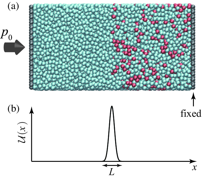
Figure 1: (a) Simulation setup of two fluid reservoirs separated by a membrane. (b) Illustration of the energy barrier $\mathcal{U}(x)$ felt only by the solute particles (red).

II.2 MD simulations

In the present study, we validate the theoretical predictions for the reflection coefficient by means of MD simulations. We use a system of identical Lennard-Jones particles for the fluid mixture with a potential barrier model for the membrane, similar to that considered in Ref. 23. Whereas they use a cubic box made of the semi-permeable membrane, here we consider a more direct geometrical setup as shown in Fig. 1. Two reservoirs are separated by a membrane as shown in Fig. 1(a); the membrane is not visible in the figure. The left reservoir contains a pure liquid solvent, while the right reservoir is filled with a liquid solution containing solute particles. The membrane is modeled by an energy barrier $\mathcal{U}$, which acts only on the solute particles, as illustrated in Fig. 1(b). The ends of the reservoirs are closed by rigid walls consisting of an FCC lattice made of the same particles as the solvent. The left wall serves as a piston, maintaining the normal pressure in the left reservoir at $P_{L}=P_{0}$ (see below for $P_{0}$). On the other hand, the right wall is fixed, and we measure the pressure in the right reservoir $P_{R}$ from the total force acting on this wall. If the membrane is perfectly semi-permeable, i.e., there is no flux of solute particles across the membrane, then the system reaches the steady state. In the present study, the osmotic pressure is measured as the pressure difference $\Pi=P_{R}-P_{L}$; it could be measured alternatively with summing all the forces exerted on each particle by the membrane, which yields identical values. The case of incomplete semi-permeability is less straightforward and described below. Since the right wall is fixed in our setup, there is no net flux of solution; the case of finite flux of mixture across the membrane could also be simulated by controlling the permeability coefficient $\mathcal{L}_{\text{hyd}}$, e.g. by introducing a drag force acting on the solvent particles in the membrane (see Ref. 16.) For simplicity we do not consider any drag force here.

For the inter-particle interactions we assume a Lennard-Jones (LJ) potential among the solvent and solute particles: $U_{ij}(r)=4\varepsilon^{\mathrm{LJ}}_{ij}[(\sigma^{\mathrm{LJ}}_{ij}/r)^{12}-(\sigma^{\mathrm{LJ}}_{ij}/r)^{6}]$. The parameters for the solute-solute, solute-solvent, and solvent-solvent interactions are commonly set as $\varepsilon^{\mathrm{LJ}}_{ij}=\varepsilon^{\mathrm{LJ}}_{0}$ and $\sigma^{\mathrm{LJ}}_{ij}=\sigma^{\mathrm{LJ}}_{0}$. The mass of all the particles is $m_{0}$. Therefore, the solute and solvent particles are mechanically identical, except that the solute particles feel the energy barrier representing the membrane. The wall particles are also described by the same interaction parameter set. In presenting the simulation results using the LJ potential, we use the units normalized in terms of the LJ parameters $\varepsilon^{\mathrm{LJ}}_{0}$ and $\sigma^{\mathrm{LJ}}_{0}$, i.e., the reference length $\ell_{0}=\sigma^{\mathrm{LJ}}_{0}$, the energy $\varepsilon_{0}=\varepsilon^{\mathrm{LJ}}_{0}$, the force $f_{0}=\varepsilon_{0}/\ell_{0}$, the pressure $P_{0}=f_{0}/\ell_{0}^{2}$, and the time $\tau_{0}=\ell_{0}^{2}m_{0}/\varepsilon^{\mathrm{LJ}}_{0}$. The energy barrier $\mathcal{U}(z)$ takes the one-dimensional Gaussian form:

$$\mathcal{U}(z)=U_{0}\exp(-a(z-z_{0})^{2}),$$ (5)

where $z_{0}$ is the position of the membrane, and $U_{0}$ controls the height of the energy barrier. The thickness of the membrane is $\sim\sqrt{a}$, where $a$ is fixed at $10/\ell_{0}^{2}$. This potential is cut off at a distance $\ell_{\rm cut}$, with $\ell_{\rm cut}=4\ell_{0}$. The size of the simulation box in $y$ and $z$ is $22.7\times 22.7$ $\ell_{0}^{2}$, and typical number of particles in one reservoir is $8380$. The temperature is kept constant at $k_{\mathrm{B}}T/\varepsilon_{0}=1$ using the Nosé–Hoover thermostat in all directions, and then the density at pressure $P_{0}$ is $0.75$ $\ell_{0}^{-3}$. The time integration is carried out with the time step $0.005\tau_{0}$. For the actual MD implementation, the open-source code LAMMPS is used throughout the paper. lam

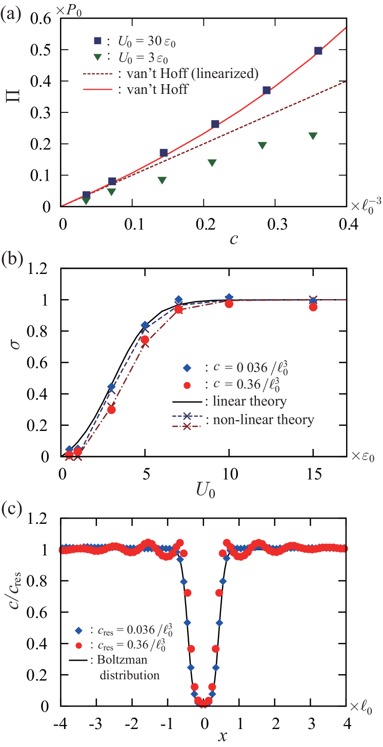
Figure 2: (a) Osmotic pressure $\Pi$ versus solute concentration $c$ in the right reservoir. The symbols indicate the MD results, and the solid line indicates the van ’t Hoff type formula given in Eq. (6). The linearized van ’t Hoff law is shown by the dashed line. (b) Reflection coefficient $\sigma$ versus height of the energy barrier $U_{0}$. The MD results are shown by the symbols. While the solid line is the theory for the low concentration regime given in Eq. (4), the dashed line and dash-dotted line are the results of the generalized theory (Eq. (3)). (c) Stationary concentration profiles across the membrane, for the case of $U_{0}=5\varepsilon_{0}$; here, the concentrations in both reservoirs are identical. The symbols indicate the MD results, which are used to calculate $\sigma$ using Eq. (3) (and plotted as crosses and lines in panel (b)). The solid line is the Boltzmann distribution.

Figure 2(a) shows the MD results of the osmotic pressure as a function of the solute concentration $c$ in the right reservoir. In the case of $U_{0}=30\,\varepsilon_{0}$, no solute particles cross the membrane during the simulation up to $5\times 10^{6}$ time steps, i.e., the membrane exhibits complete semi-permeability. In this regime, the reflection coefficient is unity, $\sigma=1$. The osmotic pressure then converges to the standard van ’t Hoff law, $\Pi=k_{\mathrm{B}}Tc$, for dilute solutions. For the larger concentrations, $\Pi$ departs from the linear line, but is still captured by the van ’t Hoff law before linearization:

$$\Pi=-\rho_{v}k_{\mathrm{B}}T\ln(1-\chi),$$ (6)

where $\chi$ is the molar fraction of the solute, $\chi=\rho_{v}^{-1}(1/c-1/\rho_{u}+1/\rho_{v})^{-1}$, and $\rho_{u}$ and $\rho_{v}$ are the density of the solute and solvent, respectively. On the other hand, when the energy barrier is small ($U_{0}=3\varepsilon_{0}$), some solute particles permeate through the membrane during the simulations. The membrane is imperfectly semi-permeable and one expects $\sigma<1$. We observe indeed that the osmotic pressure drops, coherently with $\sigma<1$. In this situation, the pressure in the right reservoir evolves with time. We accordingly compute the osmotic pressure in the following manner: after equilibration of the system at $U_{0}=30\varepsilon_{0}$ for at least $10^{5}$ time steps, we set the energy barrier at $U_{0}<30\varepsilon_{0}$. Then we average the results over $5\times 10^{5}$ time steps to evaluate the osmotic pressure.

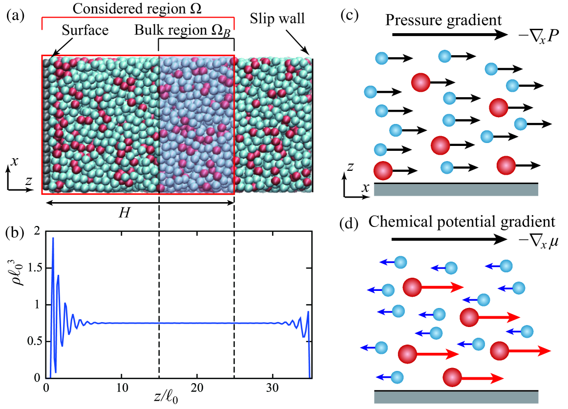
Figure 3: (a) Computational geometry for the MD simulation for an LJ mixture (solute: red, solvent: blue) in contact with a solid wall (gray). (b) Typical concentration profile along the $z$ direction. (c) Schematic illustration of the NEMD method modeling the pressure gradient. It is modeled by a force acting on each particle. (d) NEMD method for simulating the chemical potential gradient. It is modeled as a forward force per solute particle (red) and counter force per solvent particle (blue) such that the total force in the bulk is zero.

More quantitative data of the reflection coefficient $\sigma$ for the incomplete semi-permeable membrane are given in Fig. 2(b). Here, the MD values are obtained with $\sigma=\Pi/\Pi_{\mathrm{com}}$, where $\Pi_{\mathrm{com}}$ denotes the value of the complete semi-permeable case, i.e., the data shown in Fig. 2(a) for $U_{0}=30\varepsilon_{0}$. The MD results are plotted for two values of initial concentration in the right reservoir, $c=0.036/\ell_{0}^{3}$ and $c=0.36/\ell_{0}^{3}$. For comparison, the theoretical predictions quoted in Sec. II.1 are also plotted in the figure. The prediction of Eq. (4), which is valid in the dilute limit, agrees well with the MD data at $c=0.036/\ell_{0}^{3}$. For the high concentration $c=0.36/\ell_{0}^{3}$, however, the MD data departs from the prediction of Eq. (4) and takes smaller values.

The prediction of Eq. (3) is evaluated by numerically integrating the concentration profiles of the MD results. Since the solute and solvent particles considered here are mechanically identical, the mobility is independent of the concentration, and thus $\lambda$ cancels out in Eq. (3). The stationary concentration profiles are obtained at the equilibrium state, with the same concentration in the two reservoirs. Typical concentration profiles are shown in Fig. 2(c) for $U_{0}=5\varepsilon_{0}$, together with the Boltzmann distribution valid in the dilute limit, $c=c_{0}\exp(-\mathcal{U}/k_{\mathrm{B}}T)$. The deviation from the Boltzmann distribution at $c=0.36/\ell_{0}^{3}$ is a non-linear effect due to high concentration. The interaction between solute particles becomes significant, and it causes the oscillations visible in the concentration profile, similar to fluid density oscillations that generally occur near solid surfaces; Israelachvili (2011) the solute-solvent interaction causes a similar oscillation in the solvent density profile (not shown.) Taking into account this effect, Eq. (3) accurately predicts the reflection coefficient as shown in Fig. 2(b). This demonstrates the usefulness of the theoretical prediction for wide concentration ranges beyond the dilute regime, once the concentration profiles are measured or estimated.

III Non-equilibrium simulations of diffusio-osmotic flow

In this section we now consider diffusio-osmosis, i.e. the flow induced by solute gradients, but now tangential to a solid surface. We perform molecular dynamics of diffusio-osmosis for dense solute concentrations. To this end we introduce a new methodology allowing to simulate the effect of chemical potential gradients numerically.

III.1 Theory: a reminder

The geometry under consideration is shown in Fig. 3(a), with a chemical potential gradient applied parallel to the surface. In the bulk region, the total force is zero yet solute and solvent fluxes are observed. The solute concentration in a layer adjacent to the surface deviates from that in the bulk, because of either a preferential adsorption or a depletion of the solute. The force unbalance in the thin layer is the driving force of the diffusio-osmotic flow. As shown in the first paper of the series, Marbach, Yoshida, and Bocquet (2017) the fluid velocity is linearly proportional to the chemical potential gradient, according to

$$v_{x}(z)={1\over\eta}\int_{0}^{z}dz^{\prime}\,\int_{z^{\prime}}^{\infty}dz^{\prime\prime}\left(c_{\infty}-c(z^{\prime\prime})\right)\nabla_{x}\mu,$$ (7)

where $\eta$ is the fluid viscosity, $c_{\infty}$ is the concentration in the bulk region sufficiently far from the surface, and $\nabla_{x}\mu$ is the chemical potential gradient. This formula correctly recovers the classical result for the dilute solution. Anderson, Lowell, and Prieve (1982); Anderson (1989) The diffusio-osmotic mobility $K_{DO}$, relating the velocity $v_{\infty}$ far from the surface to the gradient of the chemical potential as $v_{\infty}=K_{DO}c_{\infty}\nabla_{x}\mu$, is then given by

$$K_{DO}=-\dfrac{1}{\eta}\int_{0}^{\infty}dz^{\prime}\,z^{\prime}\,\left({c(z^{\prime})\over c_{\infty}}-1\right).$$ (8)

The mobility $K_{DO}$ is negative for an excess surface concentration at the interface, i.e., the flow of solvent goes towards the low chemical potential area. Respectively, it is positive if there is a surface depletion, and the flow reverses. Note that in the case of slip at the interface with typical slip length $b$, a slip velocity adds to Eq. (7), such that $K_{DO}$ is enhanced by a factor $(1+b/L_{s})$, with $L_{s}$ the thickness of the diffusion layer. Ajdari and Bocquet (2006)

III.2 Principles for an NEMD diffusio-osmosis

In this section, our goal is to develop a method to simulate directly diffusio-osmosis on the basis of non-equilibrium MD (NEMD) simulations. This implies to generate the diffusio-osmotic flow by applying an external field that is consistent with the application of a chemical potential gradient $-\nabla_{x}\mu$. A key characteristic of diffusio-osmosis, like all interfacially driven flows – including electro- or thermo-osmosis flows Yoshida et al. (2014a); Ganti, Liu, and Frenkel (2017) –, is that it is a force-free transport phenomenon. This can be demonstrated from the fact that the hydrodynamic velocity profile is flat far away from the surface, so that all forces acting on the surface – direct interactions and hydrodynamics – do vanish in the bulk. Accordingly, if any force is applied to the system (solute+solvent), it should be balanced so that the total force acting on the fluid should vanish in the bulk region. This is obviously in contrast with the pressure driven flow. In the MD simulations, for the latter case, an external force $F_{p}$ is applied commonly to each particle in the fluid, as shown in Fig. 3(c). Bhattacharya and Lie (1989); Todd and Evans (1997); Barrat and Bocquet (1999) The applied pressure gradient, i.e., the force per volume, is then identified as $-\nabla_{x}P=F_{p}N/V$, where $N$ is the number of particles, and $V$ is the volume of the whole system $\Omega$.

To simulate diffusio-osmosis, we accordingly propose the following scheme, where we apply a differential force on the solute and on the solvent, see Fig. 3(d):

• an external force $F_{\mu}$ is applied to each solute particle in the whole system $\Omega$.

• a counter force $-[N^{B}_{s}/(N^{B}-N^{B}_{s})]F_{\mu}$ is applied to each solvent particle in $\Omega$, where $N^{B}_{s}$ and $N^{B}$ are respectively the number of solute particles and the total number of particles in the bulk region.

Note that the bulk region, denoted by $\Omega_{B}$, is defined as a volume far from the wall such that the density (and concentration) profile is flat, as depicted in Fig. 3(b). The counter force therefore ensures the force balance in the bulk volume $\Omega_{B}$. The external force strength is then related to the chemical potential gradient as

$$-\nabla_{x}\mu=F_{\mu}N^{B}/(N^{B}-N^{B}_{s}),$$ (9)

as is confirmed below via the Green–Kubo approach.

III.3 Validation of the NEMD scheme: Green–Kubo relationships

We now validate this methodology on the basis of the linear response theory. Indeed due to the Onsager symmetry, one expects that the same diffusio-osmotic mobility will relate two symmetric situations: on the one hand, the solvent flow under a solute chemical gradient, and on the other hand, the (excess) solute flux under a pressure drop. Ajdari and Bocquet (2006) This is expressed in the transport matrix as:

$$\left[\begin{array}[]{c}Q\\ J_{s}-c^{*}_{\infty}Q\end{array}\right]=\left[\begin{array}[]{cc}M^{QQ}&M^{QJ}\\ M^{JQ}&M^{JJ}\end{array}\right]\left[\begin{array}[]{c}-\nabla_{x}P\\ -\nabla_{x}\mu\end{array}\right],$$ (10)

where $Q$ and $J_{s}-c^{*}_{\infty}Q$ are the total (volume) flux and the excess solute flux, respectively, as described below. The off-diagonal coefficients in Eq. (10) are expected to be identical $M^{QJ}=M^{JQ}$ due to the Onsager time-reversal, symmetry relationship. Let us therefore demonstrate that our NEMD methodology complies to this symmetry relationship. We will calculate the Green–Kubo expression for both $M^{QJ}$ and $M^{JQ}$ cross coefficients.

We first remind quickly the general statements of linear response theory, i.e., on the response of an observed variable $\mathcal{B}$ to an external potential field $\mathcal{A}(\bm{x}_{i})F_{0}$, where $F_{0}$ is a constant microscopic force and $\mathcal{A}(\bm{x}_{i})$ is a function of the positions of the particles $\bm{x}_{i}$. The observed variable is expressed as $\langle\mathcal{B}\rangle=\mathcal{M}^{BA}F_{0}$, where $\langle\cdot\rangle$ is the ensemble average, and

$$\mathcal{M}^{BA}=\dfrac{1}{k_{\mathrm{B}}T}\int_{0}^{\infty}\langle\mathcal{B}(t)\dot{\mathcal{A}}(0)\rangle dt.$$ (11)

In the NEMD approach, the external field is $\mathcal{A}\times F_{\mu}$ with

$$\mathcal{A}=\sum_{i\in\mathrm{solute}}x_{i}-{N^{B}_{s}\over N^{B}-N^{B}_{s}}\sum_{i\in\mathrm{solvent}}x_{i},$$ (12)

where $x_{i}$ is the coordinate along the $x$ axis of particle number $i$. The observed variable is the total flux, i.e., $\mathcal{B}=Q(t)=(1/N)\sum_{i\in\mathrm{all}}\dot{x}_{i}$. Injecting these into the definition of $\mathcal{M}^{BA}$ gives the Green–Kubo formula for the diffusio-osmotic flow $\langle Q\rangle$ (abbreviated $Q$) generated by the NEMD scheme:

$$Q=M^{QJ}\left(\dfrac{N^{B}}{N^{B}-N^{B}_{s}}\right)F_{\mu},$$ (13)

$${\rm with}\,\,\,M^{QJ}=\dfrac{V}{k_{\mathrm{B}}T}\int_{0}^{\infty}\langle Q(t)(J_{s}-c^{*}_{\infty}Q)(0)\rangle dt.$$ (14)

Here $V$ is the volume of $\Omega$, and $c^{*}_{\infty}=\phi^{B}\rho_{\mathrm{av}}$, with $\phi^{B}=N^{B}_{s}/N^{B}$ being the molar fraction of solute in the bulk region $\Omega^{B}$, and $\rho_{\mathrm{av}}$ the density averaged over $\Omega$. The solute flux $J_{s}$ is calculated in terms of the particle velocity as $J_{s}=(1/V)\sum_{i\in\mathrm{solute}}\dot{x}_{i}$.

Similarly, in the reciprocal situation, we measure the solute flux $\mathcal{B}=J_{s}(t)-c^{*}_{\infty}Q(t)$ under a pressure gradient represented by $\mathcal{A}=\sum_{i\in\mathrm{all}}x_{i}$. We deduce the symmetric formula:

$$J_{s}-c^{*}_{\infty}Q=M^{JQ}\left(\dfrac{N}{V}\right)F_{p},$$ (15)

$${\rm with}\,\,\,M^{JQ}=\dfrac{V}{k_{\mathrm{B}}T}\int_{0}^{\infty}\langle(J_{s}-c^{*}_{\infty}Q)(t)Q(0)\rangle dt.$$ (16)

Comparing Eqs. (14) and (16), we find that $M^{QJ}=M^{JQ}$ so that the proposed scheme complies to Onsager’s reciprocal relation. Regarding $M^{QJ}$ and $M^{JQ}$ as the diffusio-osmotic transport coefficients relating the fluxes with the external fields, one may interpret that the microscopic forces $F_{\mu}$ and $F_{p}$ in terms of the thermodynamic forces:

$$-\nabla_{x}\mu=F_{\mu}{N^{B}\over N^{B}-N^{B}_{s}},$$ (17)

and similarly $-\nabla_{x}P=F_{p}N/V$.

Equation (17) indicates that, given the chemical potential gradient, the force acting on the solute particles is $F_{\mu}=-(1-\phi^{B})\nabla_{x}\mu$ and that on the solvent particles is $-[N^{B}_{s}/(N^{B}-N^{B}_{s})]F_{\mu}=\phi^{B}\nabla_{x}\mu$. Physically, while the force directly originating in $-\nabla_{x}\mu$ acts only on the solute particles, the counteracting force $\phi^{B}\nabla_{x}\mu$ applies to all the particles to ensure a vanishing net force.

III.4 Numerical validation of the NEMD methodology

We now apply this methodology in NEMD simulations. Our goals are first to highlight the implementation of the NEMD and second to validate the NEMD mobility by comparing it to the equilibrium Green–Kubo estimates.

III.4.1 Numerical details

In this section, solvent, solute, and wall particles interact via the LJ potential. While the parameters for the solute-solute, solute-solvent, solvent-solvent, and solvent-wall interactions are commonly set as $\varepsilon^{\mathrm{LJ}}_{ij}=\varepsilon^{\mathrm{LJ}}_{0}=\varepsilon_{0}$ and $\sigma^{\mathrm{LJ}}_{ij}=\sigma^{\mathrm{LJ}}_{0}=\ell_{0}$, the parameters for the solute-wall interaction $\varepsilon^{\mathrm{LJ}}_{\mathrm{solute,wall}}$ and $\sigma^{\mathrm{LJ}}_{\mathrm{solute,wall}}$ are varied to control the surface excess of solute particles. The wall particles are fixed at $z=0$, as in Fig. 3(a), on an FCC lattice with lattice constant $\sqrt{2}\ell_{0}$. In this setting, the hydrodynamic slip at the interface between the wall and the fluid is negligible. Ajdari and Bocquet (2006) An artificial reflecting wall is placed to truncate the computational domain, sufficiently far from the wall. At this reflecting wall, the incoming atoms are simply reflected with no tangential momentum transfer, i.e., the wall is a complete slip boundary. Since an artificial oscillation of density occurs in the vicinity of the reflecting boundary, we need to exclude this part from all measurements. We thus consider a specific region $\Omega$ (shown in Fig. 3(a)), that extends to typically a distance $10\ell_{0}$ from the reflecting boundary. The particle density is determined such that the normal pressure on the surface is $P_{0}$. Yoshida et al. (2014a); Yoshida and Bocquet (2016)

The lateral dimension of the simulation box is $17\ell_{0}\times 17\ell_{0}$, and the height of domain $\Omega$ is $H=25\ell_{0}$. The bulk region $\Omega_{B}$ is defined as $z\in[15,25]\ell_{0}$. The total number of fluid particles is $7424$, and the reflecting wall is typically placed at $z=35\ell_{0}$ (this position slightly depends on the interaction parameters). The LJ parameters are varied in the ranges $\varepsilon^{\mathrm{LJ}}_{\mathrm{solute,wall}}/\varepsilon^{\mathrm{LJ}}_{0}\in[0.5,1.5]$ and $\sigma^{\mathrm{LJ}}_{\mathrm{solute,wall}}/\sigma^{\mathrm{LJ}}_{0}\in[0.8,1.5]$. Two concentrations $\bar{c}=0.15/\ell_{0}^{3}$ and $0.04/\ell_{0}^{3}$ are considered, where $\bar{c}$ is the solute concentration averaged over $\Omega$. Other computational conditions, as well as notations for the reference parameters, are the same as those described in Sec. II.2.

III.4.2 NEMD results: velocity profiles

We show in Fig. 4(a) the velocity profiles obtained using the present NEMD method for different solute-wall interaction parameters. As expected the velocity profile is plug-like at a large distance from the wall, while exhibiting some structuration close to the interface. Here we introduce the solute adsorption $\Gamma$, defined as

$$\Gamma=\int_{0}^{\infty}dz^{\prime}\,\left(\dfrac{c(z^{\prime})}{c_{\infty}}-1\right),$$ (18)

which is a measure of the surface excess of solute in the layer: $\Gamma$ is positive for an excess surface concentration, and negative for a depletion. In Fig. 4, the two cases of $\Gamma=3.9\ell_{0}$ and $-0.9\ell_{0}$ are shown. The corresponding LJ parameters are $(\varepsilon^{\mathrm{LJ}}_{\mathrm{solute,wall}}/\varepsilon_{0},\sigma^{\mathrm{LJ}}_{\mathrm{solute,wall}}/\ell_{0})=(1.5,1.5)$ and $(0.5,0.8)$, respectively. The reversal of the velocity profiles is associated with a sign change of the adsorption: the flow is forward for $\Gamma=3.9\ell_{0}$ and backward for $\Gamma=-0.9\ell_{0}$.

Figure 5 plots the diffusio-osmotic mobility calculated from the relationship $K_{DO}=v_{\infty}/(c_{\infty}\nabla_{x}\mu)$ (here shown for $-\nabla\mu_{x}=0.025f_{0}$). The horizontal axis is the theoretical expression for the mobility given in Eq. (8). It depends on the local concentration profile data which we measure in the simulation, see Fig. 4(b). Clearly all the numerical values drop on the line of slope equal to unity, validating the theoretical prediction in a wide parameter range. We note that we used the value of $\eta$ calculated from pressure driven flow simulations. One may question whether it is pertinent to use this value to model the flow in the vicinity of the surface, where structuring of the fluid occurs, see Fig. 4(b). However the simulation data show that this provides a fairly accurate prediction for the diffusio-osmotic mobility, using the concentration profile (measured in the equilibrium situation) as an input.

We finally note that the theoretical predictions also allow to calculate the local velocity profiles in terms of the concentration profile, given in Eq. (7). Here, the integral in Eq. (7) is performed using the concentration profile as shown in Figs. 4(b); the integration range is truncated at $z/\ell_{0}=8\ell_{0}$, after the concentration converges to the bulk value. The comparison is shown in Fig. 4(a) as solid lines, showing again an excellent agreement with the simulation data.

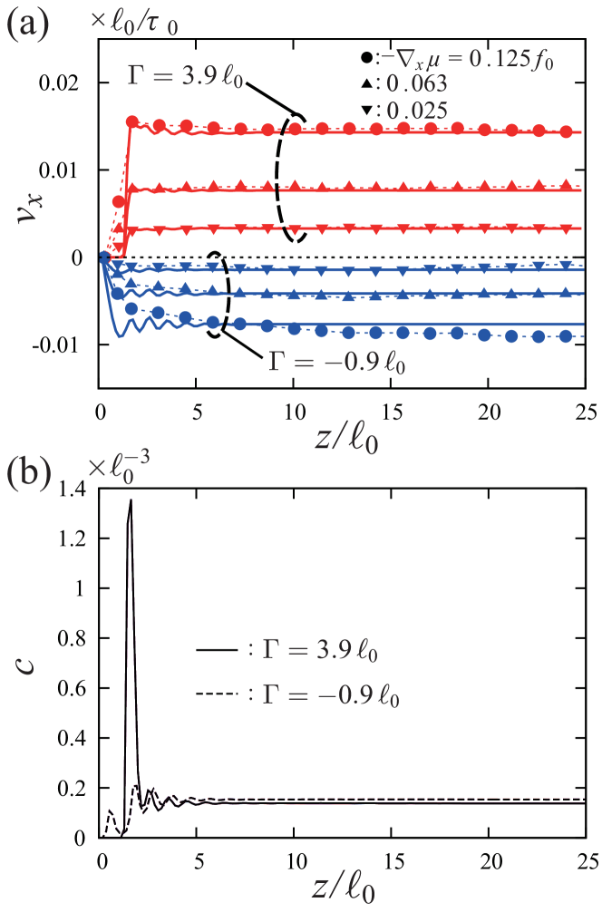
Figure 4: Velocity profiles of the diffusio-osmotic flow for the case of positive surface excess $\Gamma=3.9\ell_{0}$ and negative surface excess $\Gamma=-0.9\ell_{0}$. The average concentration is $\bar{c}=0.15/\ell_{0}^{3}$. The symbols indicate the MD results, and the solid line in panel (a) indicates the theoretical result given in Eq. (7) where we integrated the concentration profiles shown in panel (b). In panel (b), the concentration profile of $\nabla_{x}\mu=0$ is also plotted (black) in addition to the cases of $-\nabla_{x}\mu=0.025f_{0}$, $0.063f_{0}$, and $0.125f_{0}$, though the difference is negligible.

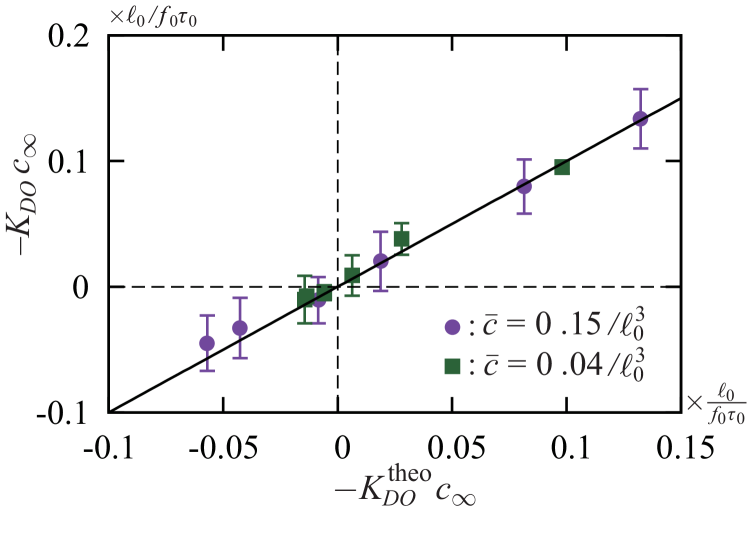
Figure 5: Numerical values of the diffusio-osmotic mobility $-K_{DO}c_{\infty}$ obtained using the NEMD method versus its theoretical counterpart $-K_{DO}^{\rm theo}c_{\infty}$ from Eq. (8). At each point at least four simulation runs have been performed and the average value is plotted, with the error bar indicating the standard deviation. The line indicating a slope equal to unity corresponds to the theoretical prediction.

III.4.3 Comparison of mobilities with equilibrium Green–Kubo estimates

As a final check, one can compare the previous values for the mobilities with those obtained from the Green–Kubo relationships in Eq. (14) and Eq. (16). One key difference is that the latter are now evaluated in equilibrium simulations.

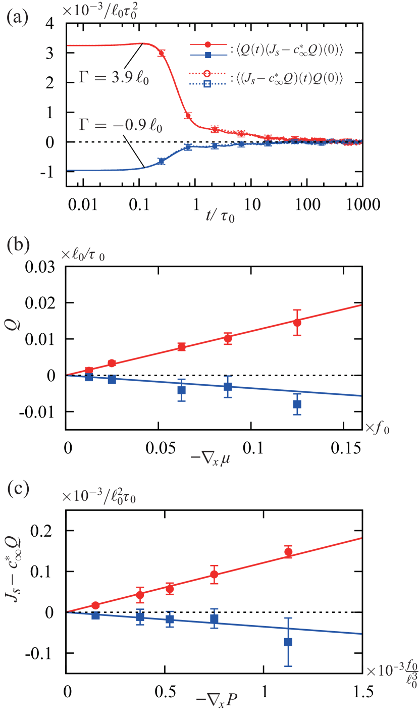
Figure 6: (a) Time correlation functions appearing in Eqs. (14) and (16), obtained using equilibrium MD simulations, for the case of $\bar{c}=0.15/\ell_{0}^{3}$. The results of ten simulation runs with different initial configurations are averaged, and the standard error is shown with the error bar. (b) Total flux $Q$ versus the chemical potential gradient $-\nabla_{x}\mu$. (c) Solute flux $J_{s}-c^{*}_{\infty}Q$ versus the pressure gradient $-\nabla_{x}P$. In panels (b) and (c), the symbols indicate the results of NEMD simulations, and the slopes of the lines indicate the coefficients obtained using Eqs. (14) and (16).

The calculated correlation functions are displayed in Fig. 6(a). The time integration appearing in Eqs. (14) and (16) suffers from significant noise, and we therefore take an average over a very large time-series sample to compute the time-correlation functions. We accordingly adopt the same strategy as in Refs. 27; 33, i.e., we perform ten independent MD simulation runs with different initial configurations, and average the time-correlation functions over the different samples and time-series. The correlations up to the time difference $t=1000\tau_{0}$ are taken, and $4.8\times 10^{6}$ time-series samples are averaged for each of ten runs.

Then the diffusio-osmotic mobility $M^{QJ}$ and the reciprocal counterpart $M^{JQ}$ are obtained by using Eqs. (14) and (16). Here, we truncate the integration range at $t=150\,\tau_{0}$ – after a sufficient decay of the correlation functions – to avoid unnecessary noise. For the example shown in Fig. 6(a), one can check that the two mobilities, calculated using the two correlation functions, do match within the numerical error, i.e., $M^{QJ}=M^{JQ}=0.12\pm 0.005\,(\ell_{0}/f_{0}\tau_{0})$ for the case of $\Gamma=3.9\ell_{0}$, and $-0.035\pm 0.005\,(\ell_{0}/f_{0}\tau_{0})$ for the case of $\Gamma=-0.9\ell_{0}$.

Finally, we show in Figs. 6(b) and (c) the comparison of the NEMD results (symbols) with the results of the Green–Kubo approach (lines). We apply various values of the chemical potential gradient $-\nabla_{x}\mu$ (tuning $F_{\mu}$), and the measured flux $Q$ is plotted in panel (b). A good agreement is obtained, which validates the direct implementation of the diffusio-osmotic flow using the present NEMD method. In panel (c), we also compare the results to the symmetric estimate of the mobility in terms of the excess solute flux under an imposed pressure gradient. The measured solute flux $J_{s}-c^{*}_{\infty}Q$ is plotted for various values of applied pressure drop $-\nabla_{x}P$ (tuning $F_{p}$). Again we find good agreement with the Green–Kubo results.

III.5 Application to the water-ethanol mixture

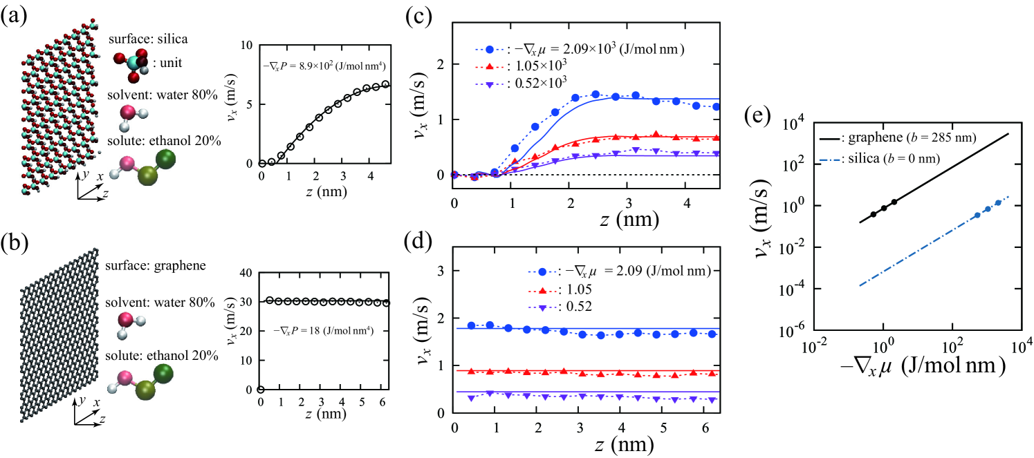
Figure 7: Illustrations of systems of water-ethanol mixture in contact with (a) silica surface and (b) graphene surface. The velocity profiles under a pressure gradient are also shown in each panel (circles), together with the continuum model (solid line); the $z$ coordinate is measured from the position of Si atoms for the silica surface, and from the C atoms for the graphene surface. The velocity profiles of the diffusio-osmotic flow are shown for the case of silica surface in (c), for the case of graphene surface in (d). The symbols indicate the MD results, and the solid lines indicate the theoretical results given in Eq. (7). The slip length is assumed to be $0$ in panel (c) and $285$ nm in panel (d). (e) Comparison of the diffusio-osmotic velocity obtained using Eq. (8). The solid line indicates the case of the graphene surface, and the dash-dotted line indicates the case of the silica surface. The dots indicate the points shown in panels (c) and (d).

We finally demonstrate the versatility of the NEMD method by applying it to more realistic systems. Here we keep the same geometry as shown in Fig. 3(a), but replace the fluid with an aqueous ethanol solution, and the wall with a silica surface (Fig. 7(a)) or a graphene sheet (Fig. 7(b)). We use the TIP4P/2005 model for water molecules, Abascal and Vega (2005) and the united atom model of the optimized potentials for liquid simulations (OPLS) Jorgensen, Madura, and Swenson (1984); Jorgensen (1986) for the ethanol molecules. The model detailed in Ref. 37 is employed for the silica surface, and the interaction parameters for the carbon atoms of the wall are extracted from the AMBER96 force field. Cornell et al. (1995) The Lorentz–Berthelot mixing rules Allen and Tildesley (1989) are used to determine the LJ parameters for the cross-interactions. The temperature is kept at $300$ K, using the Nosé–Hoover thermostat for all direction, and the pressure is at $1$ atm. The time step is set to $2$ fs. The external force is applied to each atom individually, and the value of the force per atom is obtained by dividing the force per molecule by the number of atoms within a molecule.

Here we restrict ourselves to the case of high concentration, i.e., $20$ % ethanol molar fraction, corresponding to $40$ wt% ethanol. The lateral dimension of the simulation box is $4\times 4.3$ nm², and the height of the domain $\Omega$ is $H=4.8$ nm for the case of the silica surface, and $6.3$ nm for the case of the graphene surface. The thickness of the bulk region $\Omega_{B}$ is $z\in[H-2\,\mathrm{nm},H]$.

As in the insets of Figs. 7(a) and (b), the pressure driven flow shows no velocity slip on the silica surface, and a large slip on the graphene surface. Falk et al. (2012) By fitting the formula based on the classical continuum theory, $v_{x}=(-\nabla_{x}P/2\eta)(2Hb+2Hz-z^{2})$, the slip length for the graphene surface is estimated as $b=285$ nm (see also Ref. 40). In Figs. 7(c) and (d), the diffusio-osmotic flow profiles obtained by the present NEMD are plotted. The flow velocity still shows some noise in spite of the relatively large averages at least over $100$ ns ($5\times 10^{7}$ time steps). Nevertheless, the diffusio-osmotic flows are directly observed. The theoretical predictions given in Eq. (7) are also shown in the figure, which exhibit reasonable agreement with the NEMD data. The applicability of the present NEMD method to a realistic system is thus confirmed. We note that the inverse diffusio-osmotic flow, which has been reported recently for the system of aqueous ethanol solution with a silica surface, Lee et al. (2017) was not observed in the parameter range we considered here.

We finally emphasize that the large slip length for the case of the graphene surface is accounted for by correcting Eq. (7) as remarked in Sec. III.1 (see also Refs. 26; 16.) The magnitude of the diffusio-osmotic flow is compared in Fig. 7(e), in which $v_{\infty}$ is plotted as a function of $-\nabla_{x}\mu$, using Eq. (8); the results corresponding to Fig. 7(c) and (d) are indicated by the dots. The diffusio-osmotic flow on the graphene surface is larger than that on the silica surface by about three orders of magnitude. This indicates that the hydrodynamic slip enormously enhances the diffusio-osmotic flow, as expected theoretically, see Ref. 26.

IV Summary

Transports of fluid mixtures under chemical potential difference have been investigated numerically by means of MD simulations. We first considered osmosis across membranes, and examined the reflection coefficient of imperfectly semi-permeable membranes. The theoretical expression given in Eq. (3), which we derived for high solute concentrations, was numerically validated. Next we considered the diffusio-osmotic flow near a solid-liquid interface. We introduced a novel NEMD method allowing to simulate a chemical potential gradient, involving a mixed force balance acting on solute and solvent molecules, as illustrated in Fig. 3(d). This method allows us to simulate a diffusio-osmotic flow using periodic boundary conditions. We validated the methodology on the basis of linear response theory and numerical calculations of the corresponding Green–Kubo expressions of the transport coefficients. Using the proposed NEMD method, the plug-like velocity profile was directly obtained, as shown in Figs. 4 and 7, both for the LJ fluids and water-ethanol solutions. These results showed very good agreement with the analytical predictions for both the local velocity profile and mobility. Marbach, Yoshida, and Bocquet (2017)

The proposed methodology can be extended to explore diffusio-phoretic transport involving complex molecules, like polymers, which has not been explored theoretically up to now. Further work in this direction is in progress.