Competition between stable equilibria in reaction-diffusion systems: the influence of mobility on dominance

Abstract

This paper is concerned with reaction-diffusion systems of two symmetric species in spatial dimension one, having two stable symmetric equilibria connected by a symmetric standing front. The first order variation of the speed of this front when the symmetry is broken through a small perturbation of the diffusion coefficients is computed. This elementary computation relates to the question, arising from population dynamics, of the influence of mobility on dominance, in reaction-diffusion systems modelling the interaction of two competing species. It is applied to two examples. First a toy example, where it is shown that, depending on the value of a parameter, an increase of the mobility of one of the species may be either advantageous or disadvantageous for this species. Then the Lotka–Volterra competition model, in the bistable regime close to the onset of bistability, where it is shown that an increase of mobility is advantageous. Geometric interpretations of these results are given.

1 Introduction

Reaction-diffusion systems play an important role as models for a large variety of spatio-temporal systems arising from various fields: Chemistry, Physics, Mechanics, Genetics, Ecology…. An relevant concept for the understanding of their dynamical behaviour is the dominance of equilibria, [7]: given two stable homogeneous equilibria, in which sense can one say that an equilibrium “dominates” the other one ? A possible answer is (see for instance [16]): equilibrium $A$ dominates equilibrium $B$ if there exists a travelling front connecting these two equilibria and displaying invasion of $B$ by $A$ (even if the order relation induced by this definition is not always antisymmetric, see the example in appendix, 5.2).

A natural related question is that of the influence of mobility on dominance: how is the speed of a front connecting two stable equilibria (and in particular the sign of this speed) affected by a change in the diffusion coefficients ? This question is relevant in the context of population dynamics. Consider a system modelling the evolution of densities of two species competing in a one-dimensional environment. In this case one expects the existence of two stable equilibria, each corresponding to the dominance of a species, for the local reaction system. The question above is that of the influence of the mobility of each of the two species on their relative fitness, that is on the sign of the speed of a front connecting these equilibria.

One may believe that less mobility is always advantageous, since it reduces the dispersal at the interface where the two species coexist, and thus prevents invasion (see the observations in [16]). But other effects can be invoked: an increase in the mobility of, say, the first species, changes the total density of individuals on each side of the interface, and results in undercrowding on the side where first species dominates and overcrowding on the other side, an effect having unclear consequences. While according to results of A. Hastings [13] and J. Dockery et al. [5] a heterogeneous environment seems to be always in favour of a reduction of dispersal, V. Hutson and G. T. Vickers made on a model the numerical observation that large or small diffusion cannot unambiguously be claimed to be favourable in general, [17]. More recently, L. Girardin and G. Nadin considered a Lotka–Volterra competition model close to the infinite competition limit and proved in this case a “Unity is not strength” result stating that a large dispersal is favoured, [9].

The aim of this paper is to examine on some cases the value of the first order dependence of the speed of a bistable front with respect to a perturbation of the diffusion matrix, and to try to determine the sign of this quantity. First we consider a general reaction-diffusion system in spatial dimension one, governing two symmetric scalar components, and assume the existence of two stable homogeneous equilibria that are symmetric (with respect to exchange of the two components) and connected by a symmetric (thus stationary) front. Then the symmetry between the two scalar components is broken by a small perturbation of the diffusion matrix (say a small increase of the diffusion coefficient of the first component) and several expressions are provided for the first order dependence of the speed of the front with respect to this perturbation (section 2), together with a geometric interpretation for some of these expressions. All this suggests that both signs may occur for this first order dependence, depending on the features of the initial system.

Two specific examples are then considered. First (section 3) a toy example where the initial standing front is explicit, and where it is shown that both signs (for the first order dependence introduced above) actually occur, depending on the value of a parameter of the system. This confirms on a computable case the aforementioned observations of Hutson and Vickers. The second example (treated in section 4) is the Lotka–Volterra competition model in the bistable regime, close to the onset of bistability. Using singular perturbation arguments, it is shown in this case that a large dispersal is advantageous.

2 Assumptions, notation, perturbation scheme

2.1 Setup

Let us consider the reaction-diffusion system:

$$u_{t}=F(u)+\mathcal{D}u_{xx}$$ (1)

where the time variable $t$ and the space variable $x$ are real, space domain is the full real line, the field variable $u$ is $n$-dimensional ($n$ is a positive integer), the “reaction” function $F:\mathbb{R}^{n}\rightarrow\mathbb{R}^{n}$ is smooth, and the “diffusion” matrix $\mathcal{D}$ is a positive definite symmetric $n\times n$ real matrix. Let us assume that this system admits two distinct spatially homogeneous equilibria, in other words that there exist two points $E_{-}$ and $E_{+}$ in $\mathbb{R}^{n}$ such that

$$E_{-}\not=E_{+}\quad\mbox{and}\quad F(E_{-})=F(E_{+})=0$$

and let us assume that there exists a travelling front connecting these two equilibria, in other words that there exist a smooth function $\phi:\mathbb{R}\rightarrow\mathbb{R}^{n}$ and a real quantity $c$ such that the function $(x,t)\mapsto\phi(x-ct)$ is a solution of system 1 and such that

$$\phi(\xi)\rightarrow E_{-}\quad\mbox{when}\quad\xi\rightarrow-\infty\quad\mbox{and}\quad\phi(\xi)\rightarrow E_{+}\quad\mbox{when}\quad\xi\rightarrow+\infty\,.$$

This function $\phi$ is a global solution of the system:

$$-c\phi^{\prime}(\xi)=F\bigl{(}\phi(\xi)\bigr{)}+\mathcal{D}\phi^{\prime\prime}(\xi)\,.$$ (2)

Let us assume in addition that both equilibria $E_{-}$ and $E_{+}$ are hyperbolic (that is the linear functions $DF_{E_{+}}$ and $DF_{E_{-}}$ have no eigenvalue with zero real part). In this case both functions $\xi\mapsto F\bigl{(}\phi(\xi)\bigr{)}$ and $\xi\mapsto\phi^{\prime}(\xi)$ approach $0_{\mathbb{R}^{n}}$ at an exponential rate when $\xi$ approaches $\pm\infty$, and as a consequence these functions belong to the space $L^{2}(\mathbb{R},\mathbb{R}^{n})$. Let us denote by “ $\cdot$ ” the canonical scalar product in $\mathbb{R}^{n}$, and let $\langle\cdot,\cdot\rangle_{L^{2}(\mathbb{R},\mathbb{R}^{n})}$ and $\lVert\cdot\rVert_{L^{2}(\mathbb{R},\mathbb{R}^{n})}$ denote the usual scalar product and corresponding norm in $L^{2}(\mathbb{R},\mathbb{R}^{n})$, namely (for every pair $(f,g)$ of functions of $L^{2}(\mathbb{R},\mathbb{R}^{n})$):

$$\langle f,g\rangle_{L^{2}(\mathbb{R},\mathbb{R}^{n})}=\int_{-\infty}^{+\infty}f(x)\cdot g(x)\,dx\quad\mbox{and}\quad\lVert f\rVert_{L^{2}(\mathbb{R},\mathbb{R}^{n})}=\sqrt{\langle f,f\rangle_{L^{2}(\mathbb{R},\mathbb{R}^{n})}}\,.$$

Now, it follows from system 2 that the quantity $c$ admits the following explicit expression:

$$c=-\frac{\int_{-\infty}^{+\infty}F\bigl{(}\phi(\xi)\bigr{)}\cdot\phi^{\prime}(\xi)\,d\xi}{\int_{-\infty}^{+\infty}\phi^{\prime 2}(\xi)\,d\xi}=-\frac{\langle F(\phi),\phi^{\prime}\rangle_{L^{2}(\mathbb{R},\mathbb{R}^{n})}}{\lVert\phi^{\prime}\rVert_{L^{2}(\mathbb{R},\mathbb{R}^{n})}^{2}}\,.$$ (3)

If the reaction function $F$ derives from a potential $V:\mathbb{R}^{n}\rightarrow\mathbb{R}$ (namely if $F(u)=-\nabla V(u)$ for all $u$ in $\mathbb{R}^{n}$) then this expression of $c$ becomes:

$$c=\frac{V(E_{+})-V(E_{-})}{\lVert\phi^{\prime}\rVert_{L^{2}(\mathbb{R},\mathbb{R}^{n})}^{2}}\,.$$ (4)

Thus, in this case, the sign of the speed $c$ of the front only depends on the sign of the difference between $V(E_{+})$ and $V(E_{-})$. In particular, if there exist several travelling fronts connecting $E_{-}$ to $E_{+}$, then all the velocities of these fronts have the same sign. Such is not always the case when $F$ does not derive from a potential: it is not difficult to construct an example of system of the form 1 where two distinct equilibria are connected by two travelling fronts with velocities of opposite signs (for sake of completeness such an example is given in appendix, see 5.2).

In the following we shall not assume that $F$ derives from a potential. Our aim is to understand the influence of a small change in the diffusion matrix $\mathcal{D}$ on the speed $c$ of the travelling front $\phi$.

2.2 Stability and transversality assumptions

Let us introduce the space coordinate $\xi=x-ct$ in a frame travelling at speed $c$. If two functions $u(x,t)$ and $v(\xi,t)$ are related by:

$$u(x,t)=v(\xi,t)=v(x-ct,t)\,,$$

then $u$ is a solution of system 1 if and only if $v$ is a solution of:

$$v_{t}=cv_{\xi}+F(v)+\mathcal{D}v_{\xi\xi}\,,$$ (5)

which represents system 1 rewritten in the $(\xi,t)$ coordinates system. The profile $\xi\mapsto\phi(\xi)$ of the travelling front considered in subsection 2.1 is a steady state of system 5. A small perturbation

$$(\xi,t)\mapsto\phi(\xi)+\varepsilon v(\xi,t)$$

of the profile of the front is (at first order in $\varepsilon$) a solution of 5 if and only if $v$ is a solution of the linearised system:

$$v_{t}=cv_{\xi}+DF(\phi)v+\mathcal{D}v_{\xi\xi}\,.$$ (6)

The right-hand side of 6 defines the differential operator

$$\mathcal{L}:c\partial_{\xi}+DF(\phi)+\mathcal{D}\partial_{\xi\xi}\,.$$ (7)

Considered as an unbounded operator in $L^{2}(\mathbb{R},\mathbb{R}^{n})$, it is a closed operator with dense domain $H^{2}(\mathbb{R},\mathbb{R}^{n})$. Due to translation invariance in the space variable $x$, zero is an eigenvalue of this operator; indeed, differentiating system 2 yields:

$$\mathcal{L}\phi^{\prime}=0\,.$$

Let us make the following hypotheses.

$\textup{{(H}}_{\textup{{stab-ends}}}\textup{{)}}$

The spatially homogeneous equilibria $E_{-}$ and $E_{+}$ at both ends of the front are spectrally stable for the reaction-diffusion system 1.

In other words, For every real quantity $k$, all eigenvalues of the $n\times n$ real matrices

$$DF(E_{-})-k^{2}\mathcal{D}\quad\mbox{and}\quad DF(E_{+})-k^{2}\mathcal{D}$$

have negative real parts (the subscript “stab-ends” refers to: “stable at both ends of space”). Equivalently, the essential spectrum of operator $\mathcal{L}$ is stable [14, 27].

$\textup{{(H}}_{\textup{{transv}}}\textup{{)}}$

The eigenvalue zero of the operator $\mathcal{L}$ has an algebraic multiplicity equal to $1$.

In other words, the kernel of operator $\mathcal{L}$ is reduced to $\operatorname{span}(\phi^{\prime})$, and the function $\phi^{\prime}$ does not belong to $\operatorname{Im}(\mathcal{L})$. The subscript “transv” refers to: “transverse”; indeed, this hypothesis is equivalent to the transversality of the travelling front (see 12).

The two next definitions call upon a topology on the space of travelling fronts, which may be chosen as follows: two travelling fronts $\phi_{1}$ and $\phi_{2}$ travelling at speeds $c_{1}$ and $c_{2}$ are close if: there exists a translate of $\phi_{2}$ that is close to $\phi_{1}$ (uniformly on $\mathbb{R}$), and the two speeds $c_{1}$ and $c_{2}$ are close.

Definition (isolation and robustness of the travelling front).

The travelling front $\phi$ is said to be isolated if there exists a neighbourhood of it such that every other travelling front of the same system 1 in this neighbourhood is equal to a translate of $\phi$ (and as a consequence travels at the same speed).

The travelling front $\phi$ is said to be robust if every sufficiently small perturbation of system 1 possesses a unique (up to space translation) front close to $\phi$ and travelling with a speed close to $c$.

The following statement is a rather standard transversality result [4, 3, 27, 15, 10].

Proposition 1 (isolation and robustness of $\phi$).

It follows from hypotheses $\textup{{(H}}_{\textup{{stab-ends}}}\textup{{)}}$ and $\textup{{(H}}_{\textup{{transv}}}\textup{{)}}$ that the travelling front $\phi$ under consideration is isolated and robust.

For sake of completeness a proof of this proposition is provided in 5.3.

2.3 Spectral stability

The travelling front $\phi$ is said to be spectrally stable if hypotheses $\textup{{(H}}_{\textup{{stab-ends}}}\textup{{)}}$ and $\textup{{(H}}_{\textup{{transv}}}\textup{{)}}$ are satisfied, and if moreover every nonzero eigenvalue of $\mathcal{L}$ has a negative real part. In this case the travelling front is then also non linearly stable with asymptotic phase, that is for every function $u_{0}:\mathbb{R}\rightarrow\mathbb{R}^{n}$ sufficiently close (say uniformly on $\mathbb{R}$) to a translate of $\phi$, there exists a real quantity $x_{1}$ such that the solution of system 1 with initial condition $u_{0}$ approaches the solution $(x,t)\mapsto\phi(x-x_{1}-ct)$ (at an exponential rate) when $t$ approaches $+\infty$ [14, 27].

In the two practical examples that will be considered in section 3 and section 4, the fronts under consideration will be spectrally stable indeed. However, we shall not make any additional spectral stability hypothesis at this stage since such an hypothesis is not required for the general considerations that will be made in the next subsections 2.5, 2.6, 2.7, 2.8 and 2.9.

2.4 Kernel of the adjoint linearised operator

Let $\mathcal{L}^{*}$ denote the adjoint operator of $\mathcal{L}$ for the scalar product $\langle.,.\rangle_{L^{2}(\mathbb{R},\mathbb{R}^{n})}$, that is:

$$\mathcal{L}^{*}=-c\partial_{\xi}+DF(\phi)^{*}+\mathcal{D}\partial_{\xi\xi}$$

(see figure 1).

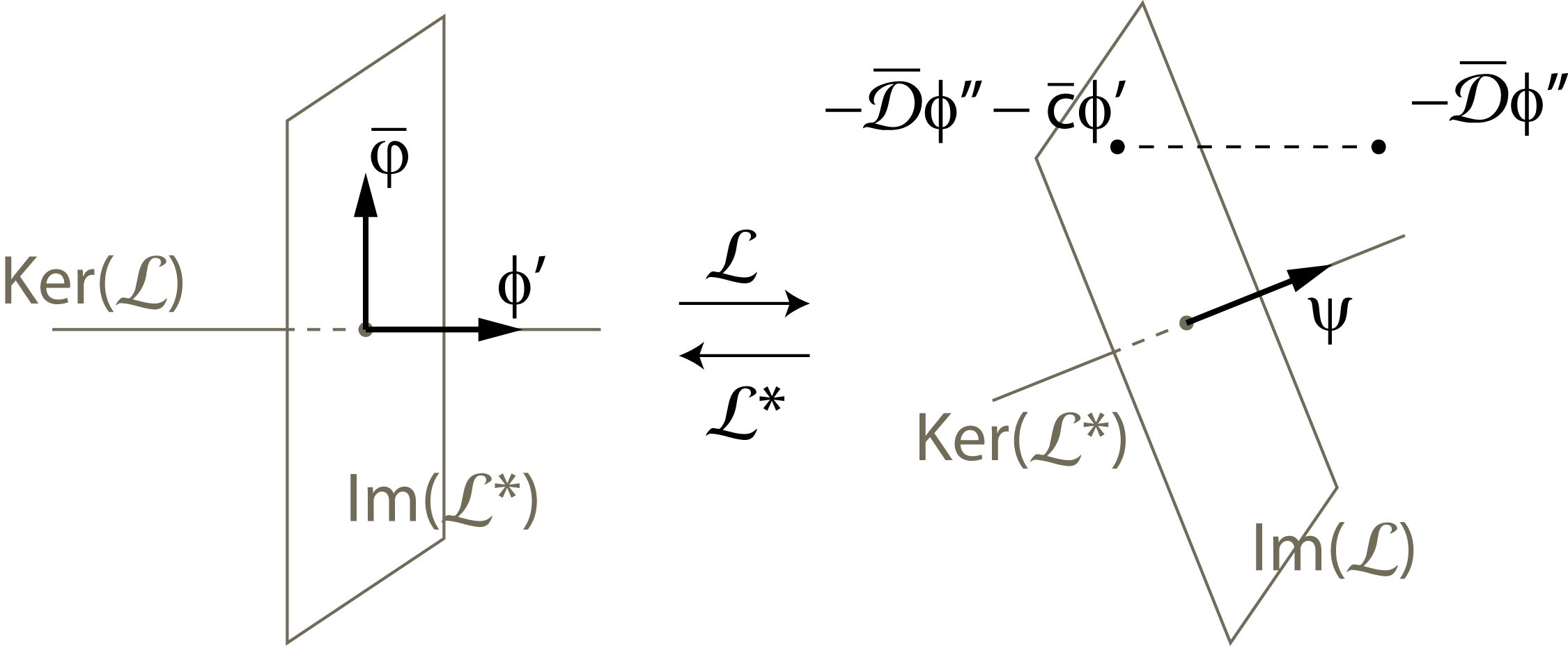
Figure 1: Notation related to the operators $\mathcal{L}$ and $\mathcal{L}^{*}$.

Hypotheses $\textup{{(H}}_{\textup{{stab-ends}}}\textup{{)}}$ and $\textup{{(H}}_{\textup{{transv}}}\textup{{)}}$ ensure that $\ker(\mathcal{L}^{*})$ is also one-dimensional [28, 27], and according to $\textup{{(H}}_{\textup{{transv}}}\textup{{)}}$ the subspaces $\ker(\mathcal{L})$ and $\ker(\mathcal{L}^{*})$ are not orthogonal to one another. As a consequence there exists a unique function $\psi$ in $\ker(\mathcal{L}^{*})$, satisfying the normalization condition

$$\langle\psi,\phi^{\prime}\rangle_{L^{2}(\mathbb{R},\mathbb{R}^{n})}=1\,,$$ (8)

and $\psi(x)$ approaches $0_{\mathbb{R}^{n}}$ at an exponential rate when $x$ approaches $\pm\infty$ [28, 27].

2.5 Perturbation of the diffusion matrix and solvency condition

Let us consider a symmetric (not necessarily positive definite) $n\times n$ real matrix $\bar{\mathcal{D}}$, a small positive quantity $\epsilon$, and the following perturbation of system 1:

$$u_{t}=F(u)+(\mathcal{D}+\epsilon\bar{\mathcal{D}})u_{xx}\,,$$ (9)

According to the consequences of hypotheses $\textup{{(H}}_{\textup{{stab-ends}}}\textup{{)}}$ and $\textup{{(H}}_{\textup{{transv}}}\textup{{)}}$ mentioned in subsection 2.2, if $\epsilon$ is sufficiently small, then the perturbed system 9 admits a unique travelling front close to $\phi$, having a speed close to $c$, and those depend smoothly on $\epsilon$. If we denote by $\phi+\epsilon\varphi$ this travelling front and by $c+\epsilon\bar{c}$ its speed, then, replacing these two ansatzes into system 9, we find that, at first order in $\epsilon$, the function $\varphi$ and the quantity $\bar{c}$ must satisfy the system

$$\mathcal{L}\varphi=-\bar{\mathcal{D}}\phi^{\prime\prime}-\bar{c}\phi^{\prime}\,.$$ (10)

Taking on both sides the scalar product by $\psi$, it follows that:

$$\bar{c}=-\langle\psi,\bar{\mathcal{D}}\phi^{\prime\prime}\rangle_{L^{2}(\mathbb{R},\mathbb{R}^{n})}\,.$$ (11)

This is a solvency condition that ensures that $-\bar{\mathcal{D}}\phi^{\prime\prime}-\bar{c}\phi^{\prime}$ is orthogonal to the kernel of $\mathcal{L}^{*}$, thus equivalently that it belongs to the image of $\mathcal{L}$ (see figure 1).

The main purpose of this paper is to investigate the sign of the quantity $\bar{c}$, since it is this sign that determines how the perturbation in 9 balances the relative dominance of the two equilibria $E_{-}$ and $E_{+}$, through the speed of the travelling front $\phi$. Indeed,

• if $\bar{c}$ is positive, then, for $\epsilon$ small positive, the influence of the perturbation will be to increase the speed of the front, thus to promote $E_{-}$ with respect to $E_{+}$;

• if conversely $\bar{c}$ is negative, then again for $\epsilon$ small positive, the influence of the perturbation will be to decrease the speed of the front, thus to promote $E_{+}$ with respect to $E_{-}$.

2.6 Alternative expression for the first order variation of the speed

We are now going to provide a second expression of $\bar{c}$ that will turn out to be useful, and in particular easier to interpret than the solvency condition 11. Since the function $-\bar{\mathcal{D}}\phi^{\prime\prime}-\bar{c}\phi^{\prime}$ belongs to the image of $\mathcal{L}$, system 10 admits exactly one solution $x\mapsto\bar{\varphi}(x)$ satisfying

$$\langle\phi^{\prime},\bar{\varphi}\rangle_{L^{2}(\mathbb{R},\mathbb{R}^{n})}=0$$

(see figure 1). Taking the scalar product by $\phi^{\prime}$ in system 10 and integrating over $\mathbb{R}$, we get

$$-\bar{c}\lVert\phi^{\prime}\rVert_{L^{2}(\mathbb{R},\mathbb{R}^{n})}^{2}=\langle\phi^{\prime},\mathcal{L}\bar{\varphi}\rangle_{L^{2}(\mathbb{R},\mathbb{R}^{n})}=\langle\mathcal{L}^{*}\phi^{\prime},\bar{\varphi}\rangle_{L^{2}(\mathbb{R},\mathbb{R}^{n})}\,,$$

and since $\mathcal{L}\phi^{\prime}=0$, the following alternative expression for $\bar{c}$ follows:

$$\bar{c}=\frac{\bigl{\langle}(\mathcal{L}-\mathcal{L}^{*})\phi^{\prime},\bar{\varphi}\bigr{\rangle}_{L^{2}(\mathbb{R},\mathbb{R}^{n})}}{\lVert\phi^{\prime}\rVert_{L^{2}(\mathbb{R},\mathbb{R}^{n})}^{2}}=\frac{\bigl{\langle}\bigl{(}DF(\phi)-DF(\phi)^{*}\bigr{)}\phi^{\prime}+2c\phi^{\prime\prime},\bar{\varphi}\bigr{\rangle}_{L^{2}(\mathbb{R},\mathbb{R}^{n})}}{\lVert\phi^{\prime}\rVert_{L^{2}(\mathbb{R},\mathbb{R}^{n})}^{2}}\,.$$ (12)

A geometrical interpretation of this expression will be given below in a more specific case.

Remark.

If $F(.)$ derives from a potential and $c=0$, then each one among expressions 11 and 12 yields $\bar{c}=0$. Indeed, in this case, $DF(\phi)$ equals $DF(\phi)^{*}$ and $c$ equals $0$ and $\mathcal{L}$ equals $\mathcal{L}^{*}$, thus:

• it follows directly from 12 that $\bar{c}=0$;

• or it follows from $\mathcal{L}=\mathcal{L}^{*}$ that $\psi$ and $\phi^{\prime}$ are proportional, thus (since $\bar{\mathcal{D}}$ is assumed to be symmetric) 11 yiels $\bar{c}=0$.

2.7 Case of a two-dimensional reaction system with symmetries

Now let us consider a more specific situation, assuming that the reaction system is two-dimensional, and that the two “species” under consideration are completely symmetric for this system, before the perturbation. Thus, keeping the notation and assumptions of the previous subsections, let us assume in addition that the dimension $n$ of the field variable $u$ equals two. Let us denote by $(u_{1},u_{2})$ the canonical coordinates of a vector $u$ in $\mathbb{R}^{2}$, let $\mathcal{S}$ denote the orthogonal symmetry exchanging the coordinates in $\mathbb{R}^{2}$, namely

$$\mathcal{S}:(u_{1},u_{2})\mapsto(u_{2},u_{1})\,,$$

and, from now on, let us make the following hypotheses:

(H3)

$F\circ\mathcal{S}=\mathcal{S}F\quad\mbox{and}\quad\mathcal{D}\mathcal{S}=\mathcal{S}\mathcal{D}\quad\mbox{and, for all $x$ in $\mathbb{R}$,}\quad\phi(-x)=\mathcal{S}\phi(x)\,.$

In other words, we assume that both the reaction-diffusion system and the front $\phi(.)$ are $u_{1}\leftrightarrow u_{2}$-symmetric.

Lemma 1 ($c$ equals $0$).

The speed $c$ equals $0$.

In other words, the front $\phi$ is a standing front.

Proof.

For every real quantity $x$, system 2 considered at $-x$ reads

$$-c\phi^{\prime}(-x)=F\bigl{(}\phi(-x)\bigr{)}+\mathcal{D}\phi^{\prime\prime}(-x)$$

and this yields, according to (H3),

$$c\mathcal{S}\phi^{\prime}(x)=\mathcal{S}F\bigl{(}\phi(x)\bigr{)}+\mathcal{S}\mathcal{D}\phi^{\prime\prime}(x)\,,$$

and finally, getting rid of $\mathcal{S}$ in this equality and comparing with system 2 considered at $x$, it follows that $c\phi^{\prime}(x)$ equals $0$, and this proves Lemma 1. ∎

Thus the operators $\mathcal{L}$ and $\mathcal{L}^{*}$ reduce to:

$$\mathcal{L}=DF(\phi)+\mathcal{D}\partial_{\xi\xi}\quad\mbox{and}\quad\mathcal{L}^{*}=DF(\phi)^{*}+\mathcal{D}\partial_{\xi\xi}\,.$$

Since the matrix $\bar{\mathcal{D}}$ is not assumed to be $u_{1}\leftrightarrow u_{2}$-symmetric (in other words we do not assume that $\bar{\mathcal{D}}\mathcal{S}=\mathcal{S}\bar{\mathcal{D}}$), the perturbation in 9 in general breaks the $u_{1}\leftrightarrow u_{2}$-symmetry. For all $u$ in $\mathbb{R}^{2}$, let us denote by $\operatorname{rot}F(u)$ the infinitesimal rotation of the vector field $F$. This quantity can be defined by:

$$DF(u)-DF(u)^{*}=\begin{pmatrix}0&-\operatorname{rot}F(u)\\ \operatorname{rot}F(u)&0\end{pmatrix}\,.$$ (13)

With this notation, expression 12 becomes:

$$\bar{c}=\frac{\int_{-\infty}^{+\infty}\operatorname{rot}F\bigl{(}\phi(x)\bigr{)}\cdot\bigl{(}\phi^{\prime}(x)\wedge\bar{\varphi}(x)\bigr{)}\,dx}{\int_{-\infty}^{+\infty}\phi^{\prime 2}(x)\,dx}=\frac{\bigl{\langle}\operatorname{rot}F(\phi),\phi^{\prime}\wedge\bar{\varphi}\bigr{\rangle}_{L^{2}(\mathbb{R},\mathbb{R}^{n})}}{\lVert\phi^{\prime}\rVert_{L^{2}(\mathbb{R},\mathbb{R}^{n})}^{2}}\,.$$ (14)

2.8 Geometric interpretation of the first order variation of the speed

The last expression 14 of $\bar{c}$ admits the following geometrical interpretation. Let us denote by $\Phi$ the image (the trajectory) in $\mathbb{R}^{2}$ of the standing front $\phi$, that is:

$$\Phi=\{\phi(x):x\in\mathbb{R}\}\subset\mathbb{R}^{2}\,.$$

The infinitesimal rotation $\operatorname{rot}F(\phi)$ measures the “shear” induced locally along $\Phi$ by the antisymmetric part of $DF$, and the real quantity $\phi^{\prime}\wedge\bar{\varphi}$ is determined by the component of the perturbation $\bar{\varphi}$ that is orthogonal to $\Phi$ (see figure 2). The shear induced by $F$ acts on this transverse perturbation (it “pushes” towards $E_{-}$ or $E_{+}$, as illustrated on figure 2), and this results in a change for the speed that is given at first order in $\epsilon$ by the quantity $\bar{c}$ defined above.

Figure 2: Geometrical illustration of expression 14 of $\bar{c}$.

2.9 Reduction using symmetry

The aim of this subsection is to take into account the symmetries (H3) of the system to simplify expressions 11 and 14 of $\bar{c}$ (that is, to write the integrals in these expressions as integrals on $\mathbb{R}_{+}$ only, instead of $\mathbb{R}$). The first symmetries on the terms involved in these integrals are stated in the following lemma.

Lemma 2 (symmetries of $\operatorname{rot}F$ and $\psi$).

For every real quantity $x$,

$$\operatorname{rot}F\bigl{(}\phi(-x)\bigr{)}=-\operatorname{rot}F\bigl{(}\phi(x)\bigr{)}\quad\mbox{and}\quad\psi(-x)=-\mathcal{S}\psi(x)\,.$$ (15)

Proof.

It follows from the symmetry of $F$ with respect to $\mathcal{S}$ in (H3) that, for every $u$ in $\mathbb{R}^{2}$,

$$F(\mathcal{S}u)=\mathcal{S}F(u)\quad\mbox{thus}\quad DF_{\mathcal{S}u}\mathcal{S}=\mathcal{S}DF_{u}\quad\mbox{and}\quad DF_{\mathcal{S}u}=\mathcal{S}DF_{u}\mathcal{S}\,,$$

and since $\mathcal{S}^{*}$ equals $\mathcal{S}$,

$$DF_{\mathcal{S}u}^{*}=\mathcal{S}DF_{u}^{*}\mathcal{S}\,.$$

It follows that

$$DF_{\mathcal{S}u}-DF_{\mathcal{S}u}^{*}=\mathcal{S}(DF_{u}-DF_{u}^{*})\mathcal{S}$$

and according to the definition 13 of $\operatorname{rot}F(\cdot)$ it follows that

$$\operatorname{rot}F(\mathcal{S}u)=-\operatorname{rot}F(u)\,.$$

Thus, for every real quantity $x$, still according to (H3),

$$\operatorname{rot}F\bigl{(}\phi(-x)\bigr{)}=\operatorname{rot}F\bigl{(}\mathcal{S}\phi(x)\bigr{)}=-\operatorname{rot}F\bigl{(}\phi(x)\bigr{)}\,.$$

and this proves the first equality of 15.

To prove the second equality, let us consider the function $\eta$ defined by: $\eta(x)=\psi(-x)$. Then, according to the expression of $\mathcal{L}^{*}$ and to hypotheses (H3),

$$\mathcal{L}^{*}(\mathcal{S}\eta)(x) =\mathcal{D}\mathcal{S}\psi^{\prime\prime}(-x)+DF^{*}\bigl{(}\phi(x)\bigr{)}\mathcal{S}\psi(-x)$$

$$=\mathcal{S}\mathcal{D}\psi^{\prime\prime}(-x)+DF^{*}\bigl{(}\mathcal{S}\phi(-x)\bigr{)}\mathcal{S}\psi(-x)$$

$$=\mathcal{S}\Bigl{(}\mathcal{D}\psi^{\prime\prime}(-x)+DF^{*}\bigl{(}\phi(-x)\bigr{)}\psi(-x)\Bigr{)}$$

$$=\mathcal{S}(\mathcal{L}^{*}\psi)(-x)$$

$$=0\,.$$

In other words, the function $x\mapsto\mathcal{S}\psi(-x)$ belongs to the eigenspace associated to the eigenvalue $0$ for the operator $\mathcal{L}^{*}$. Since this eigenspace is one-dimensional and contains the nonzero function $\psi$, it follows that there exists a real quantity $\lambda$ such that, for every real quantity $x$,

$$\mathcal{S}\psi(-x)=\lambda\psi(x)\,,$$

and since the map

$$L^{2}(\mathbb{R},\mathbb{R}^{2})\rightarrow L^{2}(\mathbb{R},\mathbb{R}^{2}),\quad f\mapsto\bigl{(}x\mapsto\mathcal{S}f(-x)\bigr{)}$$

is an involution, it follows that $\lambda=\pm 1$. According to the symmetry of $\phi$ with respect to $\mathcal{S}$ in (H3), for every real quantity $x$,

$$\phi^{\prime}(-x)=-\mathcal{S}\phi^{\prime}(x)\quad\mbox{and}\quad\psi(-x)=\lambda\mathcal{S}\psi(x)\,.$$

This shows $\lambda$ cannot be equal to $1$, or else the function $x\mapsto\psi(x)\cdot\phi^{\prime}(x)$ would be odd, and the scalar product $\langle\psi,\phi^{\prime}\rangle_{L^{2}(\mathbb{R},\mathbb{R}^{n})}$ would vanish, whereas according to the assumptions we made this scalar product must be nonzero (and was actually normalized to $1$). Thus $\lambda$ equals $-1$, and this proves the second equality of 15. Lemma 2 is proved. ∎

Since we are interested in the effect of breaking the $u_{1}\leftrightarrow u_{2}$-symmetry of the diffusion matrix, it is convenient to assume that the $u_{1}\leftrightarrow u_{2}$-symmetric part of the (symmetric) matrix $\bar{\mathcal{D}}$ vanishes (and that the $u_{1}\leftrightarrow u_{2}$-antisymmetric part of the same matrix does not vanish). This is exactly the meaning of our next hypothesis:

(H4)

$\mathcal{S}\bar{\mathcal{D}}=-\bar{\mathcal{D}}\mathcal{S}$ and $\bar{\mathcal{D}}\not=0$.

According to this hypothesis, there exists a nonzero real quantity $d$ such that:

$$\bar{\mathcal{D}}=\begin{pmatrix}d&0\\ 0&-d\end{pmatrix}\,.$$

This hypothesis leads to the following additional symmetry.

Lemma 3 (symmetry of $\bar{\varphi}$).

For every real quantity $x$,

$$\bar{\varphi}(-x)=-\mathcal{S}\bar{\varphi}(x)\,.$$

Proof.

Since $\bar{\varphi}$ is a solution of system 10, for every real quantity $x$,

$$\mathcal{D}\bar{\varphi}^{\prime\prime}(x)+DF\bigl{(}\phi(x)\bigr{)}\bar{\varphi}(x)=-\bar{\mathcal{D}}\phi^{\prime\prime}(x)-\bar{c}\phi^{\prime}(x)\,.$$

Multiplying (to the left) by $\mathcal{S}$ both sides of this equality and using the symmetries (H3) and (H4), it follows that

$$\mathcal{D}\mathcal{S}\bar{\varphi}^{\prime\prime}(x)+DF\bigl{(}\phi(-x)\bigr{)}\mathcal{S}\bar{\varphi}(x)=\bar{\mathcal{D}}\phi^{\prime\prime}(-x)+\bar{c}\phi^{\prime}(-x)\,,$$

and this shows that the function $x\mapsto-\mathcal{S}\bar{\varphi}(-x)$ is also a solution of system 10. Observe in addition that according to the symmetry of $\phi$ this solution is orthogonal to $\phi^{\prime}$ for the $L^{2}(\mathbb{R},\mathbb{R}^{n})$-scalar product. Thus this solution must be equal to $\bar{\varphi}$, and this proves the lemma. ∎

Lemma 4 (even integrands).

The three functions

$$x\mapsto\psi(x)\cdot\bar{\mathcal{D}}\phi^{\prime\prime}(x)\quad\mbox{and}\quad x\mapsto\phi^{\prime}(x)^{2}\quad\mbox{and}\quad x\mapsto\operatorname{rot}F\bigl{(}\phi(x)\bigr{)}\cdot\bigl{(}\phi^{\prime}(x)\wedge\bar{\varphi}(x)\bigl{)}$$

are even.

Proof.

For the two first functions, the symmetry follows from (H3) and Lemma 2. For the third function, observe that, for every real quantity $x$, according to (H3) and Lemma 3,

$$\phi^{\prime}(-x)\wedge\bar{\varphi}(-x)=\mathcal{S}\phi^{\prime}(x)\wedge\mathcal{S}\bar{\varphi}(x)=-\phi^{\prime}(x)\wedge\bar{\varphi}(x)\,.$$

and the result follows from Lemma 2. ∎

It follows from Lemma 4 that expressions 11 and 14 of $\bar{c}$ can be rewritten with integrals restricted to $\mathbb{R}_{+}$, namely:

$$\bar{c} =-2\int_{0}^{+\infty}\psi(x)\cdot\bar{\mathcal{D}}\phi^{\prime\prime}(x)\,dx=-2\langle\psi,\bar{\mathcal{D}}\phi^{\prime\prime}\rangle_{L^{2}(\mathbb{R}_{+},\mathbb{R}^{n})}$$ (16)

$$=\frac{\int_{0}^{+\infty}\operatorname{rot}F\bigl{(}\phi(x)\bigr{)}\cdot\bigl{(}\phi^{\prime}(x)\wedge\bar{\varphi}(x)\bigr{)}\,dx}{\int_{0}^{+\infty}\phi^{\prime 2}(x)\,dx}=\frac{\langle\operatorname{rot}F(\phi),\phi^{\prime}\wedge\bar{\varphi}\rangle_{L^{2}(\mathbb{R}_{+},\mathbb{R}^{n})}}{\lVert\phi^{\prime}\rVert_{L^{2}(\mathbb{R}_{+},\mathbb{R}^{n})}^{2}}\,.$$ (17)

The aim of the two following sections is to compute the sign of the quantity $\bar{c}$ on two specific examples.

3 Toy example

3.1 Definition

The aim of this section is to show on a toy example that both signs can occur for the quantity $\bar{c}$. Let $u=(u_{1},u_{2})$ denote again the canonical coordinates in $\mathbb{R}^{2}$, let $\mu$ denote a real quantity (a parameter), and let us consider the following system (see figure 3):

Figure 3: Phase space of the reaction system $u_{t}=F_{\mu}(u)$ for $\mu>0$.

$$u_{t}=F_{\mu}(u)+u_{xx}\quad\mbox{with}\quad F_{\mu}(u)=F_{\mu}\begin{pmatrix}u_{1}\\ u_{2}\end{pmatrix}=\begin{pmatrix}u_{1}\bigl{(}1-(u_{1}+u_{2})-\mu u_{2}(u_{2}-u_{1})\bigr{)}\\ u_{2}\bigl{(}1-(u_{1}+u_{2})-\mu u_{1}(u_{1}-u_{2})\bigr{)}\end{pmatrix}.$$ (18)

Both axes $\{u_{2}=0\}$ and $\{u_{1}=0\}$ are invariant under the reaction system $u_{t}=F_{\mu}(u)$, and the restriction of this system to each of these axes is nothing but the logistic equation: $w_{t}=w(1-w)$. Besides, the $u_{1}\leftrightarrow u_{2}$-symmetry $F_{\mu}\circ\mathcal{S}=\mathcal{S}F_{\mu}$ clearly holds.

Notation.

Let us consider the following alternative coordinate system $v=(v_{T},v_{L})$ related to $u=(u_{1},u_{2})$ by:

$$\left\{\begin{aligned} v_{T}&=u_{1}+u_{2}\\ v_{L}&=-u_{1}+u_{2}\end{aligned}\right.\Longleftrightarrow\left\{\begin{aligned} u_{1}&=\frac{v_{T}-v_{L}}{2}\\ u_{2}&=\frac{v_{T}+v_{L}}{2}\end{aligned}\right.$$ (19)

(see figure 3). The subscripts “$T$” and “$L$” refer to the adjectives “transversal” and “longitudinal”, with respect to the standing front $\phi$ that will be defined below. Along this section and the next one, these subscripts will always be used to denote the coordinates of a point in this “transversal-longitudinal” coordinate system, whereas the subscripts “$1$” and “$2$” will always be used to denote the canonical coordinates.

When expressed within the transversal-longitudinal coordinate system, system 18 takes the form

$$v_{t}=G_{\mu}(v)+v_{xx}\quad\mbox{with}\quad G_{\mu}(v)=G_{\mu}(v_{T},v_{L})=\begin{pmatrix}v_{T}-v_{T}^{2}\\ v_{L}\Bigl{(}1-v_{T}+\frac{\mu}{2}(v_{T}^{2}-v_{L}^{2})\Bigr{)}\end{pmatrix}\,.$$ (20)

According to this expression, the line $\{v_{T}=1\}$ is invariant (and transversely attractive), and the restriction of system 20 to this line reads:

$$\partial_{t}v_{L}=\frac{\mu}{2}v_{L}(1-v_{L}^{2})+\partial_{xx}v_{L}\,.$$

Thus, if the parameter $\mu$ is negative, the reaction system is monostable, with a unique stable equilibrium $E_{0}$ at $(v_{T},v_{L})=(1,0)$, whereas if $\mu$ is positive then it is bistable, with two stable equilibria $E_{1}$ at $(v_{T},v_{L})=(1,-1)$ and $E_{2}$ at $(v_{T},v_{L})=(1,1)$, and a saddle $E_{0}$ at $(v_{T},v_{L})=(1,0)$ (see figure 3). By the way,

$$DF_{\mu}(E_{1})=\begin{pmatrix}-1&1+\mu\\ 0&-\mu\end{pmatrix},\quad DF_{\mu}(E_{2})=\begin{pmatrix}-\mu&0\\ 1+\mu&-1\end{pmatrix},\quad DG_{\mu}(E_{0})=\begin{pmatrix}-1&0\\ 0&\frac{\mu}{2}\end{pmatrix}$$ (21)

(compare with expression 34 for the Lotka–Volterra competition system).

3.2 Standing front

Let us assume from now on that $\mu$ is positive (bistable case). In this case there exists for systems 18 and 20 a standing front $x\mapsto\phi(x)$ connecting $E_{1}$ to $E_{2}$, which is given (in transversal-longitudinal coordinates) by the explicit formula:

$$\phi_{T}(x)\equiv 1\quad\mbox{and}\quad\phi_{L}(x)=\tanh\frac{\sqrt{\mu}x}{2}$$ (22)

(the connection with the notation used in section 2 is obvious: equilibria $E_{1}$ and $E_{2}$ defined above correspond to equilibria $E_{-}$ and $E_{+}$ of section 2, respectively).

This standing front satisfies the $u_{1}\leftrightarrow u_{2}$-symmetry, that is $\phi(-x)=\mathcal{S}\phi(x)$ for every real quantity $x$. All the symmetry hypotheses (H3) are therefore satisfied for the system 18 and the standing front $\phi$.

For the remaining of section 3 we shall mainly work with the transversal-longitudinal coordinate system. The linear operator $\mathcal{L}$ (obtained by linearising system 20 around this standing front) reads, expressed in these coordinates,

$$\mathcal{L}\begin{pmatrix}\varphi_{T}\\ \varphi_{L}\end{pmatrix}=\begin{pmatrix}-1&0\\ (\mu-1)\phi_{L}&\frac{\mu}{2}(1-3\phi_{L}^{2})\end{pmatrix}\begin{pmatrix}\varphi_{T}\\ \varphi_{L}\end{pmatrix}+\begin{pmatrix}\varphi_{T}^{\prime\prime}\\ \varphi_{L}^{\prime\prime}\end{pmatrix}\,.$$ (23)

Lemma 5 (spectral stability of the standing front, toy example).

The standing front
$x\mapsto\phi(x)$ is spectrally stable.

Proof.

According to expressions 21, the essential spectrum of $\mathcal{L}$ is the interval:

$$(-\infty,\max(-1,-\mu)]\quad\mbox{included in}\quad(-\infty,0)\,.$$

A function

$$x\mapsto\varphi(x)=\bigl{(}\varphi_{T}(x),\varphi_{L}(x)\bigr{)}$$

is an eigenfunction of $\mathcal{L}$ for an eigenvalue $\lambda$ if and only if $\varphi_{T}$ vanishes identically and $\varphi_{L}$ is an eigenfunction of the operator

$$\ell_{\mu}:\varphi_{L}\mapsto\frac{\mu}{2}(1-3\phi_{L}^{2})\varphi_{L}+\varphi_{L}^{\prime\prime}$$ (24)

for the same eigenvalue $\lambda$. The function $x\mapsto\varphi^{\prime}_{L}(x)$ is an eigenfunction of $\ell_{\mu}$ for the eigenvalue zero (this comes from translation invariance in space), and by a standard Sturm–Liouville argument ([1]), this eigenvalue is simple and all other eigenvalues (they are real since $\ell_{\mu}$ is a self-adjoint operator for the $L^{2}(\mathbb{R},\mathbb{R})$-scalar product) are negative. Lemma 5 is proved. ∎

3.3 First order variation of the front speed

According to the notation of subsection 2.1, $\mathcal{D}=\operatorname{Id}_{\mathbb{R}^{2}}$. Let us choose the perturbation matrix $\bar{\mathcal{D}}$ as follows:

$$\bar{\mathcal{D}} =\begin{pmatrix}1&0\\ 0&-1\end{pmatrix}\mbox{ in canonical coordinates,}$$ (25)

$$\mbox{or equivalently }\bar{\mathcal{D}} =\begin{pmatrix}0&-1\\ -1&0\end{pmatrix}\mbox{ in transversal-longitudinal coordinates.}$$

All hypotheses (H1-4) of section 2 are satisfied. Let us keep the notation $\mathcal{L}^{*}$ and $\psi$ and $\bar{c}$ and $\bar{\varphi}$ introduced there. The following result shows that both signs for $\bar{c}$ may occur, depending on the value of $\mu$.

Proposition 2 (sign of the first order variation of front speed, toy example).

The
sign of $\bar{c}$ equals that of $1-\mu$; that is,

$$\bar{0}<\bar{c} \mbox{if}\quad 0<\mu<1\,,$$

$$\mbox{and}\quad\bar{c}=0 \mbox{if}\quad\mu=1\,,$$

$$\mbox{and}\quad\bar{c}<0 \mbox{if}\quad 1<\mu\,.$$

This proposition can be understood as follows.

• For $\mu$ in $(0,1)$, the perturbation promotes $E_{1}$. And since the perturbation increases the mobility of the species corresponding to $E_{1}$, this shows that an increase of mobility is advantageous in this case.

• For $\mu$ larger than $1$, the perturbation promotes $E_{1}$. And for the same reason, this time, an increase of mobility turns out to be disadvantageous.

Before proving this proposition, let us begin with a geometrical interpretation (this interpretation will by the way provide an informal proof, and make the proof easier to follow).

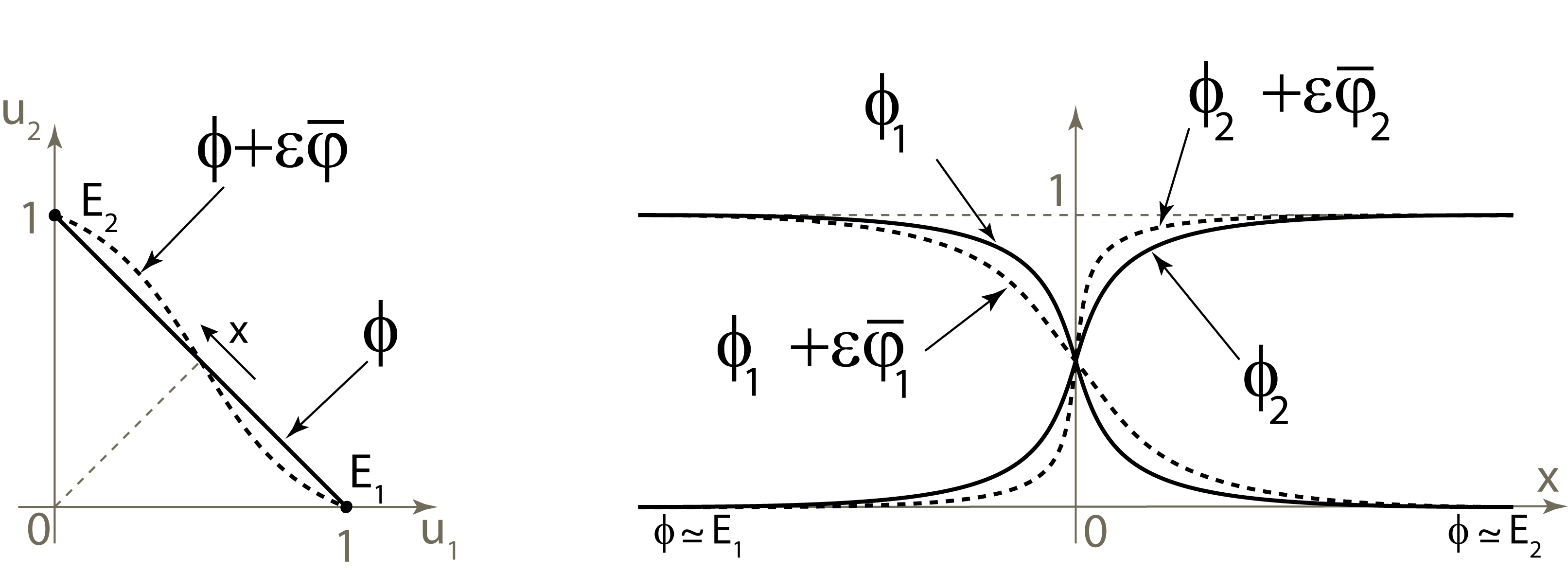
Figure 4: Left: the initial standing front $\phi$ and its perturbation $\phi+\epsilon\bar{\varphi}$. Right: the graphs of the components of these two fronts in the canonical coordinate system. The perturbation consists in an increase of the mobility of the first species (equilibrium $E_{1}$) and a decrease of the mobility of the second species (equilibrium $E_{2}$).

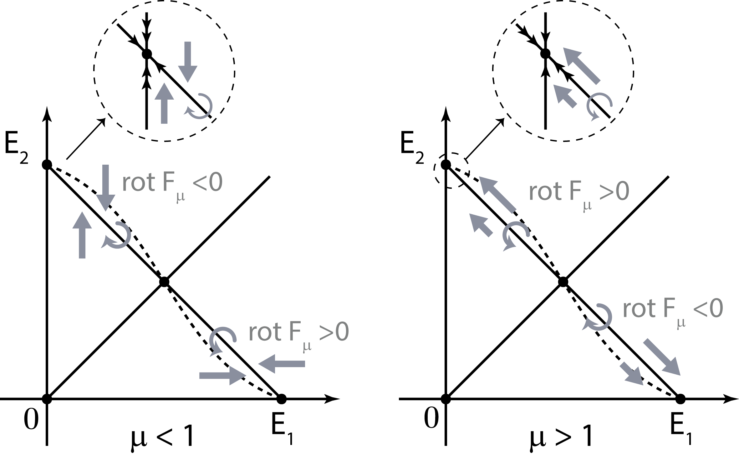
Figure 5: Orientation of the shear along the standing front in the “moderately strong” ($\mu$ smaller than $1$) versus “hard” ($\mu$ larger than $1$) competition regimes. In the moderately strong competition regime, being more mobile is an advantage, and the most mobile species (the first one, equilibrium $E_{1}$) wins with respect to the second species (equilibrium $E_{2}$). In the the hard competition regime, being more mobile is a disadvantage, and the most mobile species (the first one) looses.

Let $(\phi_{1},\phi_{2})$ denote the components of $\phi$ in the canonical coordinate system, and let $(\bar{\varphi}_{1},\bar{\varphi}_{2})$ denote the components of $\bar{\varphi}$ in the same canonical coordinate system. As illustrated on figure 4, the functions $\phi_{1}$ and $\phi_{2}$ are symmetric. The perturbation breaks this symmetry: the mobility of the first species has been slightly increased, while the mobility of the second species has been slightly decreased. As a consequence, one expects that the graph of $\phi_{1}+\epsilon\bar{\varphi}_{1}$ will be slightly flatter than that of $\phi_{1}$, and conversely that the graph of $\phi_{2}+\epsilon\bar{\varphi}_{2}$ will be slightly straighter than that of $\phi_{2}$ (figure 4). As a consequence, the position of the image of the perturbed front with respect to the image of the initial standing front should be as illustrated on figure 4; it suggests that $\bar{\varphi}_{T}(x)$ — the first component of $\bar{\varphi}$ in the transversal-longitudinal coordinate system — should be negative for $x$ negative and positive for $x$ positive (the proof below will confirm this).

On the other hand, expression 20 of the reaction-diffusion system in the transversal-longitudinal coordinate system yields, or all $x$ in $\mathbb{R}$:

$$\operatorname{rot}F_{\mu}\bigl{(}\phi(x)\bigr{)}=(\mu-1)\phi_{L}(x)\,.$$ (26)

Thus the sign of the shear induced by $F_{\mu}$ along $\phi$ depends on the sign of $\mu-1$ (see figure 5). In view of figures 4 and 5, it could be expected that, for $\mu<1$, the perturbation is in favour of $E_{1}$, while for $\mu>1$ it is in favour of $E_{2}$, as stated by Proposition 2.

Here is another possible interpretation. The parameter $\mu$ represents a sort of “intensity” of the competition between the two species. If $\mu$ is positive but smaller than $1$, the intensity can be qualified as “moderately strong”. In this case, as illustrated on figure 5 (see the zoom on equilibrium $E_{2}$), the dominant effect of the reaction term is to balance the total density $u_{1}+u_{2}$ (to drive this total density to $1$), and this turns out to be in favour of the most mobile species. On the other hand, if $\mu$ is larger than $1$, then the intensity of the competition can be qualified as “hard”. It this case, the dominant effect of the reaction term is to drive the system in favour of the most represented species locally (and away of the $E_{0}$ saddle equilibrium where both densities are equal). And this turns out to be in favour of the less mobile species. In short (you may apply this to you everyday life ): if the struggle is moderate, spread away to gain new territories; if it is bloody, avoid the dispersal and concentrate your forces !

Let us now prove Proposition 2. Let us denote by $(\psi_{T},\psi_{L})$ and by $(\bar{\varphi}_{T},\bar{\varphi}_{L})$ the transversal-longitudinal coordinates of the functions $\psi$ and $\bar{\varphi}$. To prove Proposition 2, each one among expressions LABEL:s_cond_rr_plus,c_rot_rr_plus can be used (resulting in two different proofs). The two proofs are given below, beginning with the proof involving expression 17, since it is closer to the geometrical interpretation above.

Proof using expression 17.

According to expression 17, the sign of $\bar{c}$ is equal to the sign of:

$$\int_{0}^{+\infty}\operatorname{rot}F_{\mu}\bigl{(}\phi(x)\bigr{)}\cdot\bigl{(}\phi^{\prime}(x)\wedge\bar{\varphi}(x)\bigr{)}\,dx\,.$$ (27)

According to expression 26 of $\operatorname{rot}F_{\mu}\bigl{(}\phi(x)\bigr{)}$ and expression 22 of $\phi_{L}(x)$ the function $\operatorname{rot}F_{\mu}\bigl{(}\phi(\cdot)\bigr{)}$ is of the sign of $\mu-1$ on $\mathbb{R}_{+}$.

On the other hand, since $\phi_{T}^{\prime}$ is identically zero, the function $\phi^{\prime}\wedge\bar{\varphi}$ equals $-\phi^{\prime}_{L}\bar{\varphi}_{T}$, and according to expression 22 of $\phi_{L}(x)$ the function $\phi_{L}^{\prime}$ is positive on $\mathbb{R}_{+}$. It remains to determine the sign of $\bar{\varphi}_{T}$ on $\mathbb{R}_{+}$. Projecting system 10 on the $v_{T}$-axis yields:

$$\bar{\varphi}_{T}^{\prime\prime}=\phi_{L}^{\prime\prime}+\bar{\varphi}_{T}\,.$$ (28)

Recall that according to 3, the quantities $\bar{\varphi}(-x)$ and $-\mathcal{S}\bar{\varphi}(x)$ are equal for every $x$ in $\mathbb{R}$; as a consequence, since the transversal coordinate is unchanged by $\mathcal{S}$, the quantity $\bar{\varphi}_{T}(0)$ must vanish. Since $\bar{\varphi}_{T}(x)$ approaches $0$ when $x$ approaches $+\infty$ and since according to 22 $\phi^{\prime\prime}_{L}(x)$ is negative for all $x$ in $\mathbb{R}_{+}^{*}$, it follows from equation 28 shows that the function $\bar{\varphi}_{T}$ is positive on $\mathbb{R}_{+}^{*}$ (see 10 in appendix). It follows that the function $\phi^{\prime}\wedge\bar{\varphi}$ is negative on $\mathbb{R}_{+}^{*}$, and this proves Proposition 2. ∎

Proof using expression 16.

According to expression 16, we have:

$$\bar{c}=-2\int_{0}^{+\infty}\psi(x)\cdot\bar{\mathcal{D}}\phi^{\prime\prime}(x)\,dx=2\int_{0}^{+\infty}\psi_{T}(x)\cdot\phi^{\prime\prime}_{L}(x)\,dx\,,$$

and we know from the explicit expression 22 of $\phi_{L}$ that the quantity $\phi^{\prime\prime}_{L}(x)$ is negative for all $x$ in $\mathbb{R}_{+}^{*}$. Therefore all we have to do is show that $\psi_{T}$ and $\mu-1$ have the same sign (and vanish at the same time).

According to the expression 23 of $\mathcal{L}$, system $\mathcal{L}^{*}\psi=0$ reads (using the notation $\ell_{\mu}$ introduced in definition 24):

$$-\psi_{T}+(\mu-1)\phi_{L}\psi_{L}+\psi_{T}^{\prime\prime} =0\,,$$ (29)

$$\ell_{\mu}\psi_{L} =0\,.$$ (30)

Since the eigenvalue zero of $\ell_{\mu}$ is simple (see the proof of Lemma 5 above), equation 30 shows that the functions $\psi_{L}$ and $\phi^{\prime}_{L}$ must be proportional. Thus $\psi_{L}=N\phi^{\prime}_{L}$, where, according to the normalizing condition 8, the normalizing constant $N$ is:

$$N=\Bigl{(}\int_{-\infty}^{+\infty}\phi_{L}^{\prime 2}(x)\,dx\Bigr{)}^{-1}=\lVert\phi_{L}^{\prime}\rVert_{L^{2}(\mathbb{R},\mathbb{R})}^{-2}>0\,.$$

Thus, according to equation 29, the following differential equation holds for $\psi_{T}$:

$$\psi_{T}^{\prime\prime}=\psi_{T}+N(1-\mu)\phi_{L}\phi^{\prime}_{L}\,.$$ (31)

Recall that according to 2, the quantities $\psi(-x)$ and $-\mathcal{S}\psi(x)$ are equal for every $x$ in $\mathbb{R}$; as a consequence, since the transversal coordinate is unchanged by $\mathcal{S}$, the quantity $\psi_{T}(0)=0$ must vanish. Since $\psi_{T}(x)$ approaches $0$ when $x$ approaches $+\infty$, and since both quantities $\phi_{L}(x)$ and $\phi^{\prime}_{L}(x)$ are positive for all $x$ in $\mathbb{R}_{+}^{*}$, this shows that the sign of $\psi_{T}$ must remain constant and opposite to that of $1-\mu$ on $\mathbb{R}_{+}^{*}$ (see 10 in appendix), and that $\psi_{T}$ vanishes identically if $\mu$ is equal to $1$. Proposition 2 is proved. ∎

4 Bistable Lotka–Volterra competition model

4.1 Definition

Figure 6: Phase space of the reaction system in the bistable case ($\mu>0$).

Let $\mu$ denote a real quantity (a parameter) and let us consider the following reaction-diffusion system, where the reaction term is known as the Lotka–Volterra competition model (see figure 6):

$$u_{t}=F_{\mu}(u)+u_{xx}\quad\mbox{with}\quad F_{\mu}(u)=F_{\mu}(u_{1},u_{2})=\begin{pmatrix}u_{1}\bigl{(}1-u_{1}-(1+\mu)u_{2}\bigr{)}\\ u_{2}\bigl{(}1-u_{2}-(1+\mu)u_{1}\bigr{)}\end{pmatrix}\,.$$ (32)

Both axes $\{u_{2}=0\}$ and $\{u_{1}=0\}$ are invariant under the reaction differential system $u_{t}=F_{\mu}(u)$, and the restriction of this system to each of these axes is nothing but the logistic equation $w_{t}=w(1-w)$. The $u_{1}\leftrightarrow u_{2}$-symmetry $F_{\mu}\circ\mathcal{S}=\mathcal{S}F_{\mu}$ holds.

Again in this section, we are going to use the “transversal-longitudinal” coordinate system $v=(v_{T},v_{L})$ defined exactly as in definition 19. Expressed in this coordinate system, the reaction-diffusion system 32 takes the form:

$$v_{t}=G_{\mu}(v)+v_{xx}\quad\mbox{with}\quad G_{\mu}(v)=G_{\mu}(v_{T},v_{L})=\begin{pmatrix}v_{T}-v_{T}^{2}+\frac{\mu}{2}(v_{L}^{2}-v_{T}^{2})\\ v_{L}(1-v_{T})\end{pmatrix}.$$ (33)

For all $\mu$ in $\mathbb{R}\setminus\{-2,0\}$, the reaction system admits three equilibria aside from $(0,0)$ (see figure 6):

• $E_{1}$, that is: $(u_{1},u_{2})=(1,0)\Leftrightarrow(v_{T},v_{L})=(-1,1)$,

• $E_{2}$, that is: $(u_{1},u_{2})=(0,1)\Leftrightarrow(v_{T},v_{L})=(1,1)$,

• $E_{0}$, that is: $(u_{1},u_{2})=\bigl{(}1/(2+\mu),1/(2+\mu)\bigr{)}\Leftrightarrow(v_{T},v_{L})=\bigl{(}1/(1+\mu/2),0\bigr{)}$.

The differential of the reaction system reads:

$$DF_{\mu}(u_{1},u_{2})=\begin{pmatrix}1-2u_{1}-(1+\mu)u_{2}&-(1+\mu)u_{1}\\ -(1+\mu)u_{2}&1-2u_{2}-(1+\mu)u_{1}\end{pmatrix}$$

and

$$DG_{\mu}(v_{T},v_{L})=\begin{pmatrix}1-(2+\mu)v_{T}&\mu v_{L}\\ -v_{L}&1-v_{T}\end{pmatrix}$$

thus

$$DF_{\mu}(E_{1})=\begin{pmatrix}-1&-1-\mu\\ 0&-\mu\end{pmatrix},\ DF_{\mu}(E_{2})=\begin{pmatrix}-\mu&0\\ -1-\mu&-1\end{pmatrix},\ DG_{\mu}(E_{0})=\begin{pmatrix}-1&0\\ 0&\frac{\mu}{2+\mu}\end{pmatrix}.$$ (34)

For $\mu$ negative, the reaction system is monostable ($E_{0}$ is stable and $E_{2}$ and $E_{1}$ are saddles) while for $\mu$ positive it is bistable ($E_{2}$ and $E_{1}$ are stable and $E_{0}$ is a saddle). From now on, it will be assumed that:

$$\mu>0\,,$$

or in other words that the interspecific competition rate $1+\mu$ is higher than the intraspecific competition rate $1$, or in other words that the reaction system is bistable. Observe that (with the notation of section 2), the infinitesimal rotation of the vector field $G_{\mu}$ reads:

$$\operatorname{rot}G_{\mu}(v_{T},v_{L})=-(1+\mu)v_{L}\,.$$

Thus, by contrast with the toy example studied in the previous section, the sign of the shear along the trajectory of the expected front connecting $E_{1}$ to $E_{2}$ does not depend on the parameter $\mu$ (since $\mu$ is assumed to be positive). Thus in view of the observations made in the previous section we may expect that an increase of mobility is in this case always advantageous, in other words that the quantity $\bar{c}$ is positive. The aim of this section is to prove this statement when $\mu$ is altogether positive and small.

4.2 Standing front

A smooth function

$$\phi:\mathbb{R}\rightarrow\mathbb{R}^{2},\quad x\mapsto\phi(x)=\bigl{(}\phi_{T}(x),\phi_{L}(x)\bigr{)}$$

is a stationary solution of system 33 if it is a solution of

$$G_{\mu}(\phi)+\phi^{\prime\prime}=0\Longleftrightarrow\left\{\begin{aligned} \phi_{T}^{\prime\prime}&=\phi_{T}^{2}-\phi_{T}+\frac{\mu}{2}(\phi_{T}^{2}-\phi_{L}^{2})\\ \phi_{L}^{\prime\prime}&=\phi_{L}(\phi_{T}-1).\end{aligned}\right.$$ (35)

Standing or travelling bistable fronts for systems including 32 have been studied by many authors for a long time. Existence and asymptotic stability of a bistable (monotone) travelling front connecting $E_{1}$ to $E_{2}$ were first established (in a more general setting) by C. Conley and R. Gardner using topological methods and comparison principles, [8, 2].

In [20, 21], Y. Kan-on and Q. Fang proved the uniqueness of this bistable travelling front and its spectral stability (including its transversality/robustness that is the fact that the eigenvalue $0$ is simple) for Lotka–Volterra competition-diffusion systems (a class of systems including 32 and governed by three reduced parameters aside of diffusion coefficients); from these spectral properties they recovered the asymptotic stability of this bistable front. In [20], Kan-on also proved the monotonicity of the speed of the bistable front with respect to the parameters characterizing the reaction system (but not with respect to the diffusion coefficients of the two species). Further insight into the sign of the speed of the front were achieved by J-S Guo and Y-C Lin, [11]. However, here again their results are mainly concerned with the dependence of this sign with respect to the parameters of the reaction system, but not with respect to the diffusion coefficients of the two components, and little is stated about the (rather specific) case considered in this paper, where the reaction system is $u_{1}\leftrightarrow u_{2}$-symmetric, and where the sole breaking of this $u_{1}\leftrightarrow u_{2}$-symmetry comes from the diffusion coefficients.

In [9], L. Girardin and G. Nadin also studied the dependence of the front speed with respect to the coefficients of the system, and this time espescially with respect to the diffusion coefficients of the two species. Their results hold when the parameters of the system approach certain limits; for the more restricted system 32, this corresponds to the limit when $\mu$ approaches $+\infty$ (in other words, when the interspecific competition rates approach $+\infty$). Their main “Unity is not strength” theorem states that, close to this limit, it is the most mobile species that dominates the other one. Surprisingly enough, this fits with the “moderately strong” competition case of the previous toy example, but not with the “hard” competition case where by contrast it was the less motile species that was dominant.

Our purpose is to consider system 32 when the parameter $\mu$ is positive and small (thus an asymptotics completely different from the one considered by Girardin and Nadin). By contrast with the previous toy example, the standing front connecting $E_{1}$ to $E_{2}$ is (to the knowledge of the author) not given by an explicit expressions. Note that explicit expressions for standing or travelling waves of Lotka–Volterra competition-diffusion systems have been provided by various authors, for instance by M. Rodrigo and M. Mimura in [24, 25] or by N. Kudryashov and A. Zakharchenko in [23] (this latter concerning only the monostable case), but always under restrictions on the parameters, and in particular for specific values of the diffusion coefficients (not encompassing a full interval of values for the diffusion coefficients in 32).

Our strategy will therefore be to assume that the parameter $\mu$ is small and use singular perturbation arguments to get a first order approximation (in terms of $\mu$) for the standing front (6). This will lead to a first order approximation (still in terms of $\mu$) for the quantity $\bar{c}$ we are interested in and in particular to its sign that will turn out to be positive (3). Before stating and proving these approximations, some notation is required.

4.3 Notation

1. The estimates that will be computed in the remaining of this subsection will often involve the (small) quantity $\sqrt{\mu}$ (instead of $\mu$ itself). For this reason it will be convenient to have a specific notation for this quantity. Let us write:

   $$\varepsilon=\sqrt{\mu}\,.$$ (36)

   Note that this quantity $\varepsilon$ has nothing to do with the quantity $\epsilon$ introduced in section 2 and displayed on figure 4 (that one will not be used any more in the remaining of the paper).

2. The standing front and all related functions (for instance eigenfunctions) will turn out to depend slowly on the space variable $x$. For this purpose, it will sometimes be convenient to view them as functions of the space variable $y$ related to $x$ by:

   $$y=\varepsilon x\Longleftrightarrow\frac{y}{\varepsilon}=x\,.$$ (37)

3. Up to an appropriate scaling, the standing front will be given at first order by the function

   $$\theta:y\mapsto\tanh\Bigl{(}\frac{y}{2}\Bigr{)}\,.$$ (38)

   (already encountered in the toy example of section 3). This function is a solution of equation:

   $$\theta^{\prime\prime}+\frac{1}{2}\theta(1-\theta^{2})=0$$

   and the first order expansion along $\theta$ of this equation reads: $\ell\varphi=0$, where $\ell$ is the differential operator:

   $$\ell:\varphi\mapsto\varphi^{\prime\prime}+\frac{1}{2}(1-3\theta^{2})\varphi$$ (39)

   (compare with operator $\ell_{\mu}$ defined in 24).

4. A notation is needed to deal with the remaining “higher order terms” (in $\varepsilon$) that will appear in the next computations. These higher order terms are slightly more involved than just real quantities. They depend on $\varepsilon$ and $x$, they vary slowly with respect to $x$, and they approach zero at an exponential rate when $x$ approaches $\pm\infty$. This approach to zero at infinity is important since integrals over the whole real line or half-real line will be made on various occasions. Let us define the space $\mathcal{R}$ of “remaining terms” as follows. A function

   $$r:(y,\varepsilon)\mapsto r(y,\varepsilon)$$

   belong to the set $\mathcal{R}$ if there exists a positive quantity $\delta$ such that:

   • $r$ is defined and smooth on $\mathbb{R}\times[0,\delta]$,

   • for every integer $p$, the quantity

     $$\sup_{(y,\varepsilon)\in\mathbb{R}\times[0,\delta]}e^{\lvert y/2\rvert}\lvert\partial_{y}^{p}r(y,\varepsilon)\rvert$$

     is finite.

4.4 Approximation of the standing front

The following lemma makes use of the notation $\theta(\cdot)$ and $\mathcal{R}$ introduced above. Existence and uniqueness are stated in this lemma since they will be recovered automatically by the singular perturbation approach, but as mentioned above these results are well known, [8, 2, 20]. Therefore the main interest of this lemma is the approximation of the standing front that it provides.

Lemma 6 (existence of the standing front).

For every positive and sufficiently small
quantity $\varepsilon$, the Lotka–Volterra system 33 (written in transversal-longitudinal coordinates and where $\mu$ equals $\varepsilon^{2}$ — see notation 36) admits a unique standing front

$$\phi_{\varepsilon}:\mathbb{R}\rightarrow\mathbb{R}^{2},\quad x\mapsto\phi_{\varepsilon}(x)=\bigl{(}\phi_{\varepsilon,T}(x),\phi_{\varepsilon,L}(x)\bigr{)}$$

connecting $E_{1}$ to $E_{2}$, taking its values in the first quadrant for the canonical coordinates (in other words such that $\phi_{\varepsilon,T}(x)$ is larger than $\lvert\phi_{\varepsilon,L}(x)\rvert$ for every $x$ in $\mathbb{R}$), and symmetric in the sense that:

• the fist component $x\mapsto\phi_{\varepsilon,T}(x)$ is even,

• and the second component $x\mapsto\phi_{\varepsilon,L}(x)$ is odd.

In addition, there exist functions $r_{T}$ and $r_{L}$ in $\mathcal{R}$ such that, provided that $\varepsilon$ is small enough, for every real quantity $x$,

$$\phi_{\varepsilon,T}(x) =1-\frac{\varepsilon^{2}}{2}\bigl{(}1-\theta(\varepsilon x)^{2}\bigl{)}+\varepsilon^{3}r_{T}(\varepsilon x,\varepsilon)\,,$$

$$\mbox{and}\quad\phi_{\varepsilon,L}(x) =\theta(\varepsilon x)+\varepsilon r_{L}(\varepsilon x,\varepsilon)\,.$$

Remark.

This lemma probably remains true without the additional constraint that the front must lie in the first quadrant for the canonical coordinates, but the formulation above is sufficient for our purpose.

Proof.

Let $\varepsilon$ denote a (small) positive quantity. Replacing $\mu$ by $\varepsilon^{2}$, system 35 governing stationary solutions of system 33 reads:

$$G_{\mu}(\phi)+\phi^{\prime\prime}=0\Longleftrightarrow\left\{\begin{aligned} \phi_{T}^{\prime\prime}&=\phi_{T}^{2}-\phi_{T}+\frac{\varepsilon^{2}}{2}(\phi_{T}^{2}-\phi_{L}^{2})\\ \phi_{L}^{\prime\prime}&=\phi_{L}(\phi_{T}-1)\,.\end{aligned}\right.$$ (40)

The following intermediate lemma provides a priori bounds on the transversal component of the solution we are looking for. It is illustrated by 7.

Lemma 7 (a priori bound on the standing front).

Every global solution
$x\mapsto\bigl{(}\phi_{T}(x),\phi_{L}(x)\bigr{)}$ of system 40 connecting $E_{1}$ to $E_{2}$ and such that $\lvert\phi_{L}(\cdot)\rvert$ is everywhere smaller than $\phi_{T}(\cdot)$ satisfies, for every real quantity $x$,

$$1-\frac{\varepsilon^{2}}{2}<\phi_{T}(x)<1\,.$$ (41)

Proof of Lemma 7.

According to the first equation of system 40, every such solution satisfies the differential inequalities

$$\phi_{T}(\phi_{T}-1)\leq\phi_{T}^{\prime\prime}\leq\phi_{T}\bigl{(}(1+\varepsilon^{2}/2)\phi_{T}-1\bigr{)}\,.$$

Since $\phi_{T}(x)$ must approach $1$ when $x$ approaches $\pm\infty$, it follows from the left-hand inequality that, for every real quantity $x$,

$$\phi_{T}(x)<1\,,$$

and from the right-hand inequality that, for every real quantity $x$,

$$(1+\varepsilon^{2}/2)\phi_{T}(x)>1\,.$$

Inequalities 41 follow. Lemma 7 is proved. ∎

Let us pursue the proof of Lemma 6. According to Lemma 7 it is natural to express system 40 in terms of the function $\eta_{T}$ defined by:

$$\phi_{T}=1+\varepsilon^{2}\eta_{T}\,.$$

With this notation system 40 becomes

$$\left\{\begin{aligned} \eta_{T}^{\prime\prime}&=\eta_{T}+\frac{1}{2}(1-\phi_{L}^{2})+\varepsilon^{2}\bigl{(}\eta_{T}+\eta_{T}^{2}(1+\varepsilon^{2}/2)\bigr{)}\\ \phi_{L}^{\prime\prime}&=\varepsilon^{2}\eta_{T}\phi_{L}\end{aligned}\right.$$

Using the notation

$$\tilde{\eta}_{T}=\eta_{T}^{\prime}\quad\mbox{and}\quad\tilde{\phi}_{L}=\frac{1}{\varepsilon}\phi^{\prime}_{L}\,,$$

the previous system becomes

$$\left\{\begin{aligned} \eta_{T}^{\prime}&=\tilde{\eta}_{T}\\ \tilde{\eta}_{T}^{\prime}&=\eta_{T}+\frac{1}{2}(1-\phi_{L}^{2})+\varepsilon^{2}\bigl{(}\eta_{T}+\eta_{T}^{2}(1+\varepsilon^{2}/2)\bigr{)}\\ \phi_{L}^{\prime}&=\varepsilon\tilde{\phi}_{L}\\ \tilde{\phi}_{L}^{\prime}&=\varepsilon\eta_{T}\phi_{L}\end{aligned}\right.$$ (42)

This system is appropriate for a singular perturbation argument. It converges when $\varepsilon$ approaches $0$ to the “fast” system

$$\left\{\begin{aligned} \eta_{T}^{\prime}&=\tilde{\eta}_{T}\\ \tilde{\eta}_{T}^{\prime}&=\eta_{T}+\frac{1}{2}(1-\phi_{L}^{2})\\ \phi_{L}^{\prime}&=0\\ \tilde{\phi}_{L}^{\prime}&=0\end{aligned}\right.$$ (43)

for which the two-dimensional set

$$\Sigma_{0}=\bigl{\{}(\eta_{T},\tilde{\eta}_{T},\phi_{L},\tilde{\phi}_{L})\in\mathbb{R}^{4}:\eta_{T}=-\frac{1}{2}(1-\phi_{L}^{2}),\quad\tilde{\eta}_{T}=0\bigr{\}}$$

is entirely made of equilibrium points. The matrix of the linearisation of the “fast” system 43 at every point of $\Sigma_{0}$ reads:

$$\begin{pmatrix}0&1&0&0\\ 1&0&-\phi_{L}&0\\ 0&0&0&0\\ 0&0&0&0\end{pmatrix}.$$

Its eigenvalues are $-1$, $+1$, and zero with multiplicity two. Thus the dynamics of the fast system 43 is “transversely hyperbolic” at every point of the equilibrium manifold $\Sigma_{0}$. This is the required hypothesis to apply the singular perturbation machinery. The set $\Sigma_{0}$ is the graph of the function

$$H_{0}:\mathbb{R}^{2}\longrightarrow\mathbb{R}^{2},\quad(\phi_{L},\tilde{\phi}_{L})\longmapsto(\eta_{T},\tilde{\eta}_{T})=\Bigl{(}-\frac{1}{2}(1-\phi_{L}^{2}),0\Bigr{)}\,.$$

Let us consider the following subset of $\mathbb{R}^{2}$:

$$D=\mathbb{D}(0,2)=\bigl{\{}(\phi_{L},\tilde{\phi}_{L})\in\mathbb{R}^{2}:\phi_{L}^{2}+\tilde{\phi}_{L}^{2}\leq 4\bigr{\}}\,.$$ (44)

We are going to apply Fenichel’s global center manifold theorem [6, 19, 22] with this set $D$ as definition set of the maps provided by this theorem. The properties of this set that will be used are:

• it is compact, simply connected, with a smooth boundary,

• its interior contains the trajectories of the heteroclinic connections
  $y\mapsto\bigl{(}\theta(y),\pm\theta^{\prime}(y)\bigr{)}$ (see figure 7).

According to Fenichel’s global center manifold theore, for every $\varepsilon$ sufficiently close to zero, there exists a map

$$H_{\varepsilon}:D\rightarrow\mathbb{R}^{2}$$

such that the graph of $H_{\varepsilon}$ (denoted by $\Sigma_{\varepsilon}$) is locally invariant under the dynamics of 42; this means that a solution with an initial condition on $\Sigma_{\varepsilon}$ remains on $\Sigma_{\varepsilon}$ as long as $(\phi_{L},\tilde{\phi}_{L})$ remains in $D$. Moreover, the map $H_{\varepsilon}$ coincides when $\varepsilon$ equals zero with the previous definition of $H_{0}$, and $H_{\varepsilon}$ depends smoothly on $\varepsilon$. Thus there exist smooth functions $h$ and $\tilde{h}$ of three variables, defined in a neighbourhood of $D\times\{0\}$ in $\mathbb{R}^{3}$, such that for every $(\phi_{L},\tilde{\phi}_{L})$ in $D$ and $\varepsilon$ sufficiently small,

$$H_{\varepsilon}(\phi_{L},\tilde{\phi}_{L})=\Bigl{(}-\frac{1}{2}(1-\phi_{L}^{2})+\varepsilon h(\phi_{L},\tilde{\phi}_{L},\varepsilon),\varepsilon\tilde{h}(\phi_{L},\tilde{\phi}_{L},\varepsilon)\Bigr{)}\,.$$

To study the “slow” dynamics in system 42, it is convenient to introduce some notation. According to 37, let us write:

$$y=\varepsilon x\ \Leftrightarrow\ x=y/\varepsilon\quad\mbox{and}\quad\Phi_{L}(y)=\phi_{L}(y/\varepsilon)\ \Leftrightarrow\ \Phi_{L}(\varepsilon x)=\phi_{L}(x)\,.$$

With this notation, the two last equations of system 42 reduce to:

$$\Phi_{L}^{\prime\prime}=\eta_{T}\Phi_{L}$$

thus the law governing the dynamics of system 42 on the “slow” manifold $\Sigma_{\varepsilon}$ reduces to:

$$\Phi_{L}^{\prime\prime}=-\frac{1}{2}\Phi_{L}(1-\Phi_{L}^{2})+\varepsilon\Phi_{L}h(\Phi_{L},\Phi_{L}^{\prime},\varepsilon)\,.$$ (45)

At the limit $\varepsilon$ equals $0$, this equation becomes

$$\Phi_{L}^{\prime\prime}=-\frac{1}{2}\Phi_{L}(1-\Phi_{L}^{2})\,.$$ (46)

The asymptotic equation 46 admits two hyperbolic equilibria

$$(\Phi_{L},\Phi_{L}^{\prime})=(-1,0)\quad\mbox{and}\quad(\Phi_{L},\Phi_{L}^{\prime})=(1,0)$$

and two heteroclinic solutions connecting them, which are explicitly given by:

$$y\mapsto\pm\tanh\Bigl{(}\frac{y}{2}\Bigr{)}=\pm\theta(y)$$ (47)

(see figure 7).

Figure 7: Heteroclinic connections in the phase space of equation 45 or 46, and corresponding standing front for the considered system.

Using the symmetries of the “full” system 42, we are going to prove that these two heteroclinic connections persist for the (perturbed) reduced equation 45 and remain symmetric with respect to the $\phi_{L}\leftrightarrow-\phi_{L}$ symmetry inherited from the $u_{1}\leftrightarrow u_{2}$ symmetry of the initial system.

First, let us observe that for every sufficiently small positive quantity $\varepsilon$, the (perturbed) equation 45 must admit two hyperbolic equilibria $(E_{-,\varepsilon},0)$ and $(E_{+,\varepsilon},0)$, with $E_{-,\varepsilon}$ close to $-1$ and $E_{+,\varepsilon}$ close to $1$. Let us mention here that, as usual with central manifolds, the slow manifold $\Sigma_{\varepsilon}$ is not necessarily unique, but it must contain every trajectory that remains globally in a small neighbourhood of it ([6, 19, 22]). Therefore it must contain the equilibria corresponding to $E_{1}$ and $E_{2}$. It follows that $E_{-,\varepsilon}-=-1$ and $E_{+,\varepsilon}=+1$, in other words:

$$h(-1,0,\varepsilon)=h(-1,0,\varepsilon)=0\,.$$ (48)

Now, the robustness of the heteroclinic connections 47 is asserted by the following intermediate lemma.

Lemma 8 (robustness of heteroclinic connections).

For every sufficiently small positive quantity $\varepsilon$, there exists a global solution

$$y\mapsto\Phi_{\varepsilon,L}(y)$$

of the reduced equation 45 such that

$$\Phi_{\varepsilon,L}(y)\rightarrow-1\quad\mbox{when}\quad y\rightarrow-\infty\quad\mbox{and}\quad\Phi_{\varepsilon,L}(y)\rightarrow+1\quad\mbox{when}\quad y\rightarrow+\infty\,,$$

and, for every real quantity $y$,

$$\Phi_{\varepsilon,L}(-y)=-\Phi_{\varepsilon,L}(y)\,.$$

Proof.

The “full” system 42 admits two symmetries, the reversibility $x\leftrightarrow-x$ and the $\phi_{L}\leftrightarrow-\phi_{L}$ symmetry inherited from the $u_{1}\leftrightarrow u_{2}$ symmetry of the initial system. To be more precise, according to these two symmetries, if

$$x\mapsto\bigl{(}\eta_{T}(x),\tilde{\eta}_{T}(x),\phi_{L}(x),\tilde{\phi}_{L}(x)\bigr{)}$$

is a solution of system 42, then the following two functions are also solutions:

$$x\mapsto\bigl{(}\eta_{T}(-x),-\tilde{\eta}_{T}(-x),\phi_{L}(-x),-\tilde{\phi}_{L}(-x)\bigr{)}$$

and $$x\mapsto\bigl{(}\eta_{T}(x),\tilde{\eta}_{T}(x),-\phi_{L}(x),-\tilde{\phi}_{L}(x)\bigr{)}$$

It is well known that local center manifolds of systems admitting equivariant or reversibility symmetries can be chosen in such a way that those manifolds be themselves invariant under these symmetries — note that since center manifolds are not necessarily unique this is however not obvious — and as a consequence in such a way that the reduced systems (obtained by reduction of the initial systems to those symmetric local center manifolds) still admit the same symmetries as the initial system. See [26] and [18, 12] for more recent expositions, the last one concerning infinite dimensional dynamical systems. If a similar result could be invoked for global center manifolds, we would be able to choose our global center manifold $\Sigma_{\varepsilon}$ in such a way that it is invariant under the two symmetries of the full system 42, namely in such a way that:

• $h(\phi_{L},\tilde{\phi}_{L},\varepsilon)$ is even with respect to $\phi_{L}$,

• $h(\phi_{L},\tilde{\phi}_{L},\varepsilon)$ is even with respect to $\tilde{\phi}_{L}$,

• $\tilde{h}(\phi_{L},\tilde{\phi}_{L},\varepsilon)$ is odd with respect to $\phi_{L}$,

• $\tilde{h}(\phi_{L},\tilde{\phi}_{L},\varepsilon)$ is odd with respect to $\tilde{\phi}_{L}$,

and as a consequence the reduced equation 45 would admit the same two symmetries, and the conclusions of Lemma 8 would immediately follow from these symmetries. Unfortunately, to the knowledge of the author, no statement concerning the existence of global center manifolds satisfying reversibility and equivariant symmetries and applicable in our case is available in the existing litterature. However we are going to recover this symmetry for the aforementioned heteroclinic connections by another (less direct) argument.

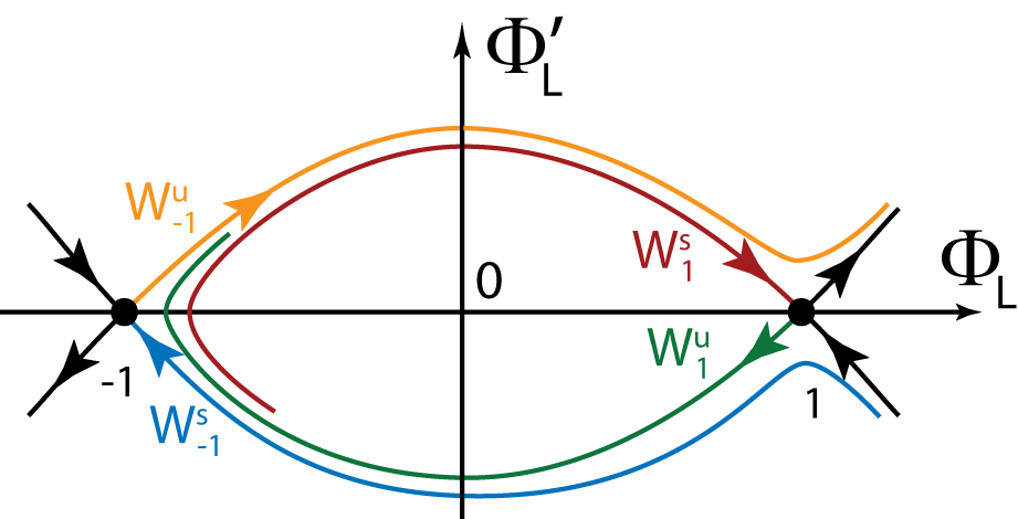
Figure 8: The four trajectories $W^{\textup{{u}}}_{-1}$ and $W^{\textup{{s}}}_{1}$ and $W^{\textup{{u}}}_{1}$ and $W^{\textup{{s}}}_{-1}$. As argued in the proof of Lemma 8, if these four trajectories differ, one of them (in this case $W^{\textup{{s}}}_{1}$) is “trapped” by the other ones.

Let us fix $\varepsilon$ (positive, small) and let us consider the four trajectories $W^{\textup{{u}}}_{-1}$ and $W^{\textup{{s}}}_{1}$ and $W^{\textup{{u}}}_{1}$ and $W^{\textup{{s}}}_{-1}$ depicted on figure 8 (they are part of the stable and unstable manifolds of $(-1,0)$ and $(1,0)$ for the reduced equation 45 for this value of $\varepsilon$). Let us proceed by contradiction and assume that $W^{\textup{{u}}}_{-1}$ and $W^{\textup{{s}}}_{1}$ do not coincide and that $W^{\textup{{u}}}_{1}$ and $W^{\textup{{s}}}_{-1}$ do not coincide. Then, by a Jordan curve argument (see figure 8), we see that at least one of those four trajectories does remains “trapped” (by the three others) in the domain $D$ defined in 44. Let

$$x\mapsto\bigl{(}\eta_{T}(x),\tilde{\eta}_{T}(x),\phi_{L}(x),\tilde{\phi}_{L}(x)\bigr{)}$$

denote a solution of the full system 42 corresponding to this trajectory. Then, due to the symmetries of this full system 42, the three functions

$$x\mapsto\bigl{(}\eta_{T}(-x),-\tilde{\eta}_{T}(-x),\phi_{L}(-x),-\tilde{\phi}_{L}(-x)\bigr{)}$$

and $$x\mapsto\bigl{(}\eta_{T}(x),\tilde{\eta}_{T}(x),-\phi_{L}(x),-\tilde{\phi}_{L}(x)\bigr{)}$$

and $$x\mapsto\bigl{(}\eta_{T}(-x),-\tilde{\eta}_{T}(-x),-\phi_{L}(-x),\tilde{\phi}_{L}(-x)\bigr{)}$$

are still solutions of the same system, and these three additional solutions still globally remain in a small neighbourhood of the center manifold $\Sigma_{\varepsilon}$. As a consequence, theses three additional solutions must also belong to $\Sigma_{\varepsilon}$, leading to a topological contradiction, see figure 8.

Thus at least one among the two pairs $(W^{\textup{{u}}}_{-1},W^{\textup{{s}}}_{1})$ and $(W^{\textup{{u}}}_{1},W^{\textup{{s}}}_{-1})$ must be reduced to a single trajectory, and by a similar argument this must actually be the case for both pairs. This proves the existence of the two heteroclinic connections. Their symmetries follows from the same argument. Lemma 8 is proved. ∎

Let us define the function $r_{L}:(y,\varepsilon)\mapsto r_{L}(y,\varepsilon)$ by:

$$\Phi_{\varepsilon,L}(y)=\theta(y)+\varepsilon r_{L}(y,\varepsilon)\,.$$

Since the eigenvalues of equilibria $(-1,0)$ and $(1,0)$ of equation 45 are close to $-1$ and $+1$, the “remaining” function $r_{L}$ belongs to the space $\mathcal{R}$ defined in subsection 4.3. Let us define the function

$$\phi_{\varepsilon}:\mathbb{R}\rightarrow\mathbb{R}^{2},\quad x\mapsto\bigl{(}\phi_{\varepsilon,T}(x),\phi_{\varepsilon,L}(x)\bigr{)}$$

by:

$$\left\{\begin{aligned} \phi_{\varepsilon,T}(x)&=1-\frac{\varepsilon^{2}}{2}(1-\phi_{\varepsilon,L}^{2})+\varepsilon^{3}h\bigl{(}\Phi_{\varepsilon,L}(\varepsilon x),\Phi_{\varepsilon,L}^{\prime}(\varepsilon x),\varepsilon\bigr{)}\,,\\ \phi_{\varepsilon,L}(x)&=\Phi_{\varepsilon,L}(\varepsilon x)\,.\end{aligned}\right.$$ (49)

This function is a standing front connecting $E_{1}$ to $E_{2}$, it is $u_{1}\leftrightarrow u_{2}$-symmetric (in other words $\phi_{\varepsilon}(-x)$ equals $\mathcal{S}\phi_{\varepsilon}(x)$ for every $x$ in $\mathbb{R}$), and it takes its values in the “first quadrant” $\phi_{T}>\lvert\phi_{L}\rvert$. In addition, if we define the “remaining” function $r_{T}$ by:

$$\phi_{\varepsilon,T}(x)=1-\frac{\varepsilon^{2}}{2}\bigl{(}1-\theta(\varepsilon x)^{2}\bigr{)}+\varepsilon^{3}r_{T}(\varepsilon x,\varepsilon)$$

then, according to equalities 48, this function $r_{T}$ belongs to $\mathcal{R}$. The proof of Lemma 6 is thus complete. ∎

4.5 First-order variation of the front speed

With the notation of section 2, the diffusion matrix $\mathcal{D}$ equals identity. Let $\varepsilon$ denote a positive quantity, sufficiently small so that 6 holds, and let us consider the standing front $\phi_{\varepsilon}(\cdot)$ provided by this lemma.

Lemma 9 (spectral stability of the standing front).

The standing front

$$x\mapsto\phi_{\varepsilon}(x)$$

is spectrally stable (in the sense of 2.3, that is including the fact that the eigenvalue $0$ has an algebraic multiplicity equal to $1$) for the Lotka–Volterra system 33.

Proof.

As mentioned in subsection 4.2, this follows from the general stability results proved by Kan-on and Fang in [20, 21]. ∎

Let us choose the perturbation matrix $\bar{\mathcal{D}}$ exactly as in the toy example considerer in section 3, see definition 25. For those items, all the hypotheses (H1-4) of section 2 are satisfied. Let us denote by

$$\mathcal{L}_{\varepsilon}\quad\mbox{and}\quad\mathcal{L}^{*}_{\varepsilon}\quad\mbox{and}\quad\psi_{\varepsilon}\quad\mbox{and}\quad\bar{c}_{\varepsilon}$$

the objects that were denoted by $\mathcal{L}$ and $\mathcal{L}^{*}$ and $\psi$ and $\bar{c}$ in section 2 (these objects now depend on $\varepsilon$), and let us again denote by $\theta$ the function: $y\mapsto\tanh(y/2)$. The aim of this subsection is to prove the following proposition.

Proposition 3 (first order variation of front speed).

The
following estimate holds:

$$\bar{c}_{\varepsilon}\ \sim_{\varepsilon\rightarrow 0^{+}}\ -\varepsilon\ \frac{\int_{0}^{+\infty}\theta(y)\theta^{\prime}(y)\theta^{\prime\prime}(y)\,dy}{\lVert\theta^{\prime}\rVert_{L^{2}(\mathbb{R}_{+},\mathbb{R})}^{2}}\,.$$ (50)

As a consequence the quantity $\bar{c}$ is positive for every sufficiently small positive quantity $\varepsilon$. In other words, for the Lotka–Volterra competition model in the bistable regime, close to the onset of bistability, an increase of mobility provides an advantage. Since in this case the competition between the two species can be qualified as “moderately strong”, we recover the interpretation given for the toy example in section 3, that is the fact that when competition is moderately strong an increase of mobility is advantageous.

Proof.

We are going to use expression 11 of $\bar{c}$, namely, according to the expression of $\bar{\mathcal{D}}$,

$$\bar{c}_{\varepsilon}=\int_{-\infty}^{+\infty}\bigl{(}\psi_{\varepsilon,T}(x)\phi_{\varepsilon,L}^{\prime\prime}(x)+\psi_{\varepsilon,L}(x)\phi_{\varepsilon,T}^{\prime\prime}(x)\bigl{)}\,dx$$ (51)

where $x\mapsto\psi_{\varepsilon}(x)=\bigl{(}\psi_{\varepsilon,T}(x),\psi_{\varepsilon,L}(x)\bigr{)}$ (written in the $v$-coordinate system) is the solution of $\mathcal{L}^{*}_{\varepsilon}\psi=0$ satisfying the normalization condition 8, namely:

$$\langle\psi_{\varepsilon},\phi_{\varepsilon}^{\prime}\rangle_{L^{2}(\mathbb{R},\mathbb{R}^{2})}=1$$ (52)

(here there would be no gain from restricting the integrals in 51 to $\mathbb{R}_{+}$ as in the reduced expression 16).

Lemma 6 provides convenient approximations for the functions $\phi_{\varepsilon,T}^{\prime\prime}(\cdot)$ and $\phi_{\varepsilon,L}^{\prime\prime}(\cdot)$, thus what remains to be done is to get similar approximations for $\psi_{\varepsilon,T}(\cdot)$ and $\psi_{\varepsilon,L}(\cdot)$. According to expression 33 of the Lotka–Volterra system in the transversal-longitudinal coordinate systems, the operator $\mathcal{L}_{\varepsilon}$ reads (in the same coordinate system):

$$\mathcal{L}_{\varepsilon}\begin{pmatrix}\varphi_{T}\\ \varphi_{L}\end{pmatrix}(x)=\begin{pmatrix}1-(2+\varepsilon^{2})\phi_{\varepsilon,T}(x)&\varepsilon^{2}\phi_{\varepsilon,L}(x)\\ -\phi_{\varepsilon,L}(x)&1-\phi_{\varepsilon,T}(x)\end{pmatrix}\begin{pmatrix}\varphi_{T}(x)\\ \varphi_{L}(x)\end{pmatrix}+\begin{pmatrix}\varphi_{T}^{\prime\prime}(x)\\ \varphi_{L}^{\prime\prime}(x)\end{pmatrix}\,.$$

Notation.

For the remaining of section 4, let us use the notation $r(\cdot,\cdot)$ to denote every function in the space $\mathcal{R}$ defined in subsection 4.3, or every $2\times 2$ or $4\times 4$ matrix having all its coefficients in this space $\mathcal{R}$. Thus each of the symbols $r(\cdot,\cdot)$ that appear in the expressions below corresponds to a (different) element of $\mathcal{R}$ or matrix of elements of $\mathcal{R}$.

With this notation and according to the approximation provided by Lemma 6, the expression above reduces to

$$\mathcal{L}_{\varepsilon}\begin{pmatrix}\varphi_{T}\\ \varphi_{L}\end{pmatrix}(x)=\begin{pmatrix}-1+\varepsilon^{2}r(y,\varepsilon)&\varepsilon^{2}\theta(y)+\varepsilon^{3}r(y,\varepsilon)\\ -\theta(y)+\varepsilon r(y,\varepsilon)&\frac{\varepsilon^{2}}{2}\bigl{(}1-\theta(y)^{2}\bigr{)}+\varepsilon^{3}r(y,\varepsilon)\end{pmatrix}\begin{pmatrix}\varphi_{T}(x)\\ \varphi_{L}(x)\end{pmatrix}+\begin{pmatrix}\varphi_{T}^{\prime\prime}(x)\\ \varphi_{L}^{\prime\prime}(x)\end{pmatrix},.$$

According to this expression the system $\mathcal{L}^{*}_{\varepsilon}\psi=0$ reads

$$\begin{pmatrix}\psi_{\varepsilon,T}^{\prime\prime}(x)\\ \psi_{\varepsilon,L}^{\prime\prime}(x)\end{pmatrix}=\begin{pmatrix}1+\varepsilon^{2}r(y,\varepsilon)&\theta(y)+\varepsilon r(y,\varepsilon)\\ -\varepsilon^{2}\theta(y)+\varepsilon^{3}r(y,\varepsilon)&-\frac{\varepsilon^{2}}{2}\bigl{(}1-\theta(y)^{2}\bigr{)}+\varepsilon^{3}r(y,\varepsilon)\end{pmatrix}\begin{pmatrix}\psi_{\varepsilon,T}(x)\\ \psi_{\varepsilon,L}(x)\end{pmatrix}$$

or equivalently

$$\begin{pmatrix}\psi_{\varepsilon,T}^{\prime\prime}(x)\\ \frac{1}{\varepsilon^{2}}\psi_{\varepsilon,L}^{\prime\prime}(x)\end{pmatrix}=\begin{pmatrix}1&\theta(y)\\ -\theta(y)&-\frac{1}{2}\bigl{(}1-\theta(y)^{2}\bigr{)}\end{pmatrix}\begin{pmatrix}\psi_{\varepsilon,T}(x)\\ \psi_{\varepsilon,L}(x)\end{pmatrix}+\varepsilon r(y,\varepsilon)\begin{pmatrix}\psi_{\varepsilon,T}(x)\\ \psi_{\varepsilon,L}(x)\end{pmatrix}\,.$$ (53)

Let us introduce the functions $\tilde{\psi}_{\varepsilon,T}(\cdot)$ and $\tilde{\psi}_{\varepsilon,L}(\cdot)$ defined by (for every real quantity $x$):

$$\tilde{\psi}_{\varepsilon,T}(x)=\psi^{\prime}_{\varepsilon,T}(x)\quad\mbox{and}\quad\tilde{\psi}_{\varepsilon,L}(x)=\frac{1}{\varepsilon}\psi_{\varepsilon,L}^{\prime}(x)\,.$$

Then the previous system becomes

$$\begin{pmatrix}\psi_{\varepsilon,T}^{\prime}\\ \tilde{\psi}_{\varepsilon,T}^{\prime}\\ \psi_{\varepsilon,L}^{\prime}\\ \tilde{\psi}_{\varepsilon,L}^{\prime}\end{pmatrix}(x)=\begin{pmatrix}0&1&0&0\\ 1&0&\theta(y)&0\\ 0&0&0&0\\ 0&0&0&0\end{pmatrix}\begin{pmatrix}\psi_{\varepsilon,T}\\ \tilde{\psi}_{\varepsilon,T}\\ \psi_{\varepsilon,L}\\ \tilde{\psi}_{\varepsilon,L}\end{pmatrix}(x)+\varepsilon r(y,\varepsilon)\begin{pmatrix}\psi_{\varepsilon,T}\\ \tilde{\psi}_{\varepsilon,T}\\ \psi_{\varepsilon,L}\\ \tilde{\psi}_{\varepsilon,L}\end{pmatrix}(x)\,.$$

Another change of variables will fire the non-diagonal term in the $4\times 4$ matrix above. For this purpose, let us introduce the functions $\eta_{\varepsilon,T}(\cdot)$ and $\tilde{\eta}_{\varepsilon,T}(\cdot)$ defined by (for every real quantity $x$):

$$\eta_{\varepsilon,T}(x)=\psi_{\varepsilon,T}(x)+\theta(y)\psi_{\varepsilon,L}(x)\quad\mbox{and}\quad\tilde{\eta}_{\varepsilon,T}(x)=\eta_{\varepsilon,T}^{\prime}(x)\,.$$ (54)

Then,

$$\tilde{\eta}_{\varepsilon,T}^{\prime}(x)=\eta_{\varepsilon,T}^{\prime\prime}(x)=\tilde{\psi}_{\varepsilon,T}^{\prime}(x)+\varepsilon^{2}\theta^{\prime\prime}(y)\psi_{\varepsilon,L}(x)+2\varepsilon^{2}\theta^{\prime}(y)\tilde{\psi}_{\varepsilon,L}(x)+\varepsilon\theta(y)\tilde{\psi}_{\varepsilon,L}^{\prime}(x)\,,$$

thus, since according to the second line of the system above the dominant term in the expression of $\tilde{\psi}_{\varepsilon,T}^{\prime}(x)$ is $\psi_{\varepsilon,T}(x)+\theta(y)\tilde{\psi}_{\varepsilon,T}(x)$ and since this dominant term equals $\eta_{\varepsilon,T}(x)$, this system can be rewritten as follows:

$$\begin{pmatrix}\eta_{\varepsilon,T}^{\prime}\\ \tilde{\eta}_{\varepsilon,T}^{\prime}\\ \psi_{\varepsilon,L}^{\prime}\\ \tilde{\psi}_{\varepsilon,L}^{\prime}\end{pmatrix}(x)=\begin{pmatrix}0&1&0&0\\ 1&0&0&0\\ 0&0&0&0\\ 0&0&0&0\end{pmatrix}\begin{pmatrix}\eta_{\varepsilon,T}\\ \tilde{\eta}_{\varepsilon,T}\\ \psi_{\varepsilon,L}\\ \tilde{\psi}_{\varepsilon,L}\end{pmatrix}(x)+\varepsilon r(y,\varepsilon)\begin{pmatrix}\eta_{\varepsilon,T}\\ \tilde{\eta}_{\varepsilon,T}\\ \psi_{\varepsilon,L}\\ \tilde{\psi}_{\varepsilon,L}\end{pmatrix}(x)\,.$$

Since the first $2\times 2$ block of the $4\times 4$ matrix of this system is hyperbolic, and since the quantities $\eta_{\varepsilon,T}(x)$ and $\tilde{\eta}_{\varepsilon,T}(x)$ and $\psi_{\varepsilon,L}(x)$ and $\tilde{\psi}_{\varepsilon,L}(x)$ must approach zero when $t$ approaches plus or minus infinity, this shows that there exist a positive quantity $C$, independent of $\varepsilon$ provided that $\varepsilon$ is sufficiently small, such that, for all $x$ in $\mathbb{R}$,

$$\lvert\eta_{\varepsilon,T}(x)\rvert\leq C\varepsilon\bigl{(}\lvert\psi_{\varepsilon,L}(x)\rvert+\lvert\tilde{\psi}_{\varepsilon,L}(x)\rvert\bigr{)}\quad\mbox{and}\quad\lvert\tilde{\eta}_{\varepsilon,T}(x)\rvert\leq C\varepsilon\bigl{(}\lvert\psi_{\varepsilon,L}(x)\rvert+\lvert\tilde{\psi}_{\varepsilon,L}(x)\rvert\bigr{)}\,.$$ (55)

Let us introduce the function $\Psi_{\varepsilon,L}(\cdot)$ defined by (for every $(x,y)$ in $\mathbb{R}^{2}$ with $y=\varepsilon x$):

$$\Psi_{\varepsilon,L}(y)=\psi_{\varepsilon,L}\Bigl{(}\frac{y}{\varepsilon}\Bigr{)}\Leftrightarrow\Psi_{\varepsilon,L}(\varepsilon x)=\psi_{\varepsilon,L}(x)\,.$$

With this notation, the second equation of system 53 becomes:

$$\Psi_{\varepsilon,L}^{\prime\prime}(y)=-\theta(y)\psi_{\varepsilon,T}\Bigl{(}\frac{y}{\varepsilon}\Bigr{)}-\frac{1}{2}\bigl{(}1-\theta(y)^{2}\bigr{)}\Psi_{\varepsilon,L}(y)+\varepsilon r(y,\varepsilon)\Psi_{\varepsilon,L}(y)$$

Thus, according to the notation 54,

$$\Psi_{\varepsilon,L}^{\prime\prime}(y)=\frac{1}{2}\bigl{(}3\theta(y)^{2}-1\bigr{)}\Psi_{\varepsilon,L}(y)-\theta(y)\eta_{\varepsilon,T}\Bigl{(}\frac{y}{\varepsilon}\Bigr{)}+\varepsilon r(y,\varepsilon)\Psi_{\varepsilon,L}(y)$$

and thus, according to inequalities 55, and up to increasing the quantity $C$, for all $y$ in $\mathbb{R}$ (using the notation $\ell$ introduced in subsection 4.3),

$$\lvert(\ell\Psi_{\varepsilon,L})(y)\rvert=\lvert\Psi_{\varepsilon,L}^{\prime\prime}(y)-\frac{1}{2}\bigl{(}3\theta(y)^{2}-1\bigr{)}\Psi_{\varepsilon,L}(y)\rvert\leq C\varepsilon\bigl{(}\lvert\Psi_{\varepsilon,L}(y)\rvert+\lvert\Psi_{\varepsilon,L}^{\prime}(y)\rvert\bigr{)}\,.$$ (56)

Let

$$\alpha=\frac{\langle\Psi_{\varepsilon,L},\theta^{\prime}\rangle_{L^{2}(\mathbb{R},\mathbb{R})}}{\lVert\theta^{\prime}\rVert_{L^{2}(\mathbb{R},\mathbb{R})}^{2}}$$

and, for all $y$ in $\mathbb{R}$, let

$$\chi_{\varepsilon,L}(y)=\Psi_{\varepsilon,L}(y)-\alpha\theta^{\prime}(y)\,.$$ (57)

By construction, the function $\chi_{\varepsilon,L}(\cdot)$ is orthogonal to $\theta^{\prime}$, that is to the kernel of $\ell$ and since $\ell\Psi_{\varepsilon,L}$ and $\ell\chi_{\varepsilon,L}$ are equal it follows from 56 that, for every real quantity $y$,

$$\lvert(\ell\chi_{\varepsilon,L})(y)\rvert\leq C\varepsilon\bigl{(}\lvert\Psi_{\varepsilon,L}(y)\rvert+\lvert\Psi_{\varepsilon,L}^{\prime}(y)\rvert\bigr{)}\,.$$

As a consequence, up to increasing the quantity $C$, for every $y$ in $\mathbb{R}$,

$$\lvert\chi_{\varepsilon,L}(y)\rvert\leq C\varepsilon\bigl{(}\lvert\Psi_{\varepsilon,L}(y)\rvert+\lvert\Psi_{\varepsilon,L}^{\prime}(y)\rvert\bigr{)}\quad\mbox{and}\quad\lvert\chi_{\varepsilon,L}^{\prime}(y)\rvert\leq C\varepsilon\bigl{(}\lvert\Psi_{\varepsilon,L}(y)\rvert+\lvert\Psi_{\varepsilon,L}^{\prime}(y)\rvert\bigr{)}\,.$$ (58)

It follows from 57 and 58 that, for every real quantity $y$,

$$(1-C\varepsilon)\bigl{(}\lvert\Psi_{\varepsilon,L}(y)\rvert+\lvert\Psi_{\varepsilon,L}^{\prime}(y)\rvert\bigr{)}\leq\alpha\bigl{(}\lvert\theta^{\prime}(y)\rvert+\lvert\theta^{\prime\prime}(y)\rvert\bigr{)}$$

and as a consequence, provided that $\varepsilon$ is sufficiently small,

$$\lvert\Psi_{\varepsilon,L}(y)\rvert+\lvert\Psi_{\varepsilon,L}^{\prime}(y)\rvert=r(y,\varepsilon)\,.$$ (59)

As a consequence, it follows from 57 and 58 that

$$\psi_{\varepsilon,L}(x)=\alpha\theta^{\prime}(\varepsilon x)+\varepsilon r(\varepsilon x,\varepsilon)\quad\mbox{and}\quad\psi_{\varepsilon,L}^{\prime}(x)=\varepsilon\alpha\theta^{\prime}(\varepsilon x)+\varepsilon^{2}r(\varepsilon x,\varepsilon)\,.$$ (60)

Besides, it follows from the upper bounds 55 and 59 that

$$\eta_{\varepsilon,T}(x)=\varepsilon r(\varepsilon x,\varepsilon)\,.$$

thus, according to the definition 54 of $\eta_{\varepsilon,T}(\cdot)$,

$$\psi_{\varepsilon,T}(x)=-\alpha\theta(\varepsilon x)\theta^{\prime}(\varepsilon x)+\varepsilon r(\varepsilon x,\varepsilon)\,.$$ (61)

The normalization condition 52 will provide the approximate value of the quantity $\alpha$. This normalization condition reads:

$$\langle\psi_{\varepsilon,T},\phi_{\varepsilon,T}^{\prime}\rangle_{L^{2}(\mathbb{R},\mathbb{R})}+\langle\psi_{\varepsilon,L},\phi_{\varepsilon,L}^{\prime}\rangle_{L^{2}(\mathbb{R},\mathbb{R})}=1\,,$$

in other words, according to the expressions of $\phi_{\varepsilon,T}(\cdot)$ and $\phi_{\varepsilon,L}(\cdot)$ provided by 6,

$$\int_{-\infty}^{+\infty}\psi_{\varepsilon,T}(x)\cdot\varepsilon^{3}r(\varepsilon x,\varepsilon)\,dx+\int_{-\infty}^{+\infty}\psi_{\varepsilon,L}(x)\cdot\bigl{(}\varepsilon\theta^{\prime}(\varepsilon x)+\varepsilon^{2}r(\varepsilon x,\varepsilon)\bigr{)}\,dx=1\,.$$

According to the expression 61, the first integral of the left-hand side of this last inequality is a $\mathcal{O}_{\varepsilon\rightarrow 0}(\varepsilon^{2})$. Thus it follows from the expression 60 for $\psi_{\varepsilon,L}(\cdot)$ that:

$$\alpha=\frac{1}{\lVert\theta^{\prime}\rVert_{L^{2}(\mathbb{R},\mathbb{R})}^{2}}+\mathcal{O}_{\varepsilon\rightarrow 0}(\varepsilon)\,.$$ (62)

We are now in position to estimate the value of $\bar{c}_{\varepsilon}$ given by 51. According to Lemma 6,

$$\phi_{\varepsilon,T}^{\prime\prime}(x)=\varepsilon^{4}r(\varepsilon x,\varepsilon)\,,$$

thus it follows from 51 and the expression 60 of $\psi_{\varepsilon,L}(\cdot)$ that

$$\bar{c}_{\varepsilon}=\mathcal{O}(\varepsilon^{3})+\int_{-\infty}^{+\infty}\,\psi_{\varepsilon,T}(x)\ \phi_{\varepsilon,L}^{\prime\prime}(x)\,dx\,,$$

thus, according to the expression of $\phi_{\varepsilon,L}(\cdot)$ provided by 6 and the expression 61 of $\psi_{\varepsilon,T}(\cdot)$,

$$\bar{c}_{\varepsilon} =\mathcal{O}(\varepsilon^{3})+\int_{-\infty}^{+\infty}\bigl{(}-\alpha\theta(\varepsilon x)\theta^{\prime}(\varepsilon x)+\varepsilon r(\varepsilon x,\varepsilon)\bigr{)}\cdot\bigl{(}\varepsilon^{2}\theta^{\prime\prime}(\varepsilon x)+\varepsilon^{3}r(\varepsilon x,\varepsilon)\bigr{)}\,dx$$

$$=\mathcal{O}(\varepsilon^{3})-\varepsilon^{2}\alpha\int_{-\infty}^{+\infty}\theta(\varepsilon x)\theta^{\prime}(\varepsilon x)\theta^{\prime\prime}(\varepsilon x)\,dx$$

$$=\mathcal{O}(\varepsilon^{3})-\varepsilon\alpha\int_{-\infty}^{+\infty}\theta(y)\theta^{\prime}(y)\theta^{\prime\prime}(y)\,dy\,.$$

Finally, according to the expression 62 for $\alpha$,

$$\bar{c}_{\varepsilon}\sim_{\varepsilon\to 0}-\frac{\varepsilon}{\lVert\theta^{\prime}\rVert_{L^{2}(\mathbb{R},\mathbb{R})}^{2}}\int_{-\infty}^{+\infty}\theta(y)\theta^{\prime}(y)\theta^{\prime\prime}(y)\,dy\,,$$

and restricting the integrals to $\mathbb{R}_{+}$ estimate 50 follows. Proposition 3 is proved. ∎

5 Appendix

5.1 An elementary property of the solutions of a second order conservative equation

Let $f:[0,+\infty)\rightarrow\mathbb{R}$ denote a continuous function satisfying

$$f(t)\rightarrow 0\quad\mbox{when}\quad t\rightarrow+\infty\quad\mbox{and}\quad f(\cdot)\mbox{ does not vanish on }(0,+\infty)\,,$$

and let us consider the following second order equation:

$$\ddot{u}=u+f\,.$$ (63)

The aim of this subsection is to prove the following lemma.

Lemma 10 (solution homoclinic to $0$).

There exists a unique solution $t\mapsto u(t)$ of equation 63 defined on $[0,+\infty)$ such that

$$u(0)=0\quad\mbox{and}\quad u(t)\rightarrow 0\quad\mbox{when}\quad t\rightarrow+\infty\,.$$ (64)

This solution does not vanish on $(0,+\infty)$, and its sign is opposite to the sign of $f(\cdot)$.

Proof.

Let $t\mapsto u(t)$ denote a solution of equation 63 on $\mathbb{R}_{+}$ and let us consider the functions $x=u+\dot{u}$ and $y=-u+\dot{u}$ (thus $u$ equals $(x-y)/2$. Those function satisfy the system

$$\dot{x} =x+f$$ (65)

$$\dot{y} =-y+f$$ (66)

Equation 66 shows that $y(t)$ approaches $0$ when $t$ approaches $+\infty$, and since the same assertion holds for $u(t)$, it must also hold for $x(t)$. Thus, according to equation 65, the function $x(\cdot)$ must be given by:

$$x(t)=-\int_{t}^{+\infty}e^{t-s}f(s)\,ds\,.$$

This provides an explicit expression for $x(0)$, thus also for $y(0)$ since $u(0)$ equals $0$, and finally for $y(t)$ for every nonnegative quantity $t$ according to 66. It follows that $u(t)$ must be equal to the following expression for every nonnegative time $t$:

$$\frac{1}{2}\biggl{(}e^{-t}\int_{0}^{t}f(s)(e^{-s}-e^{s})\,ds+(e^{-t}-e^{t})\int_{t}^{+\infty}f(s)e^{-s}\,ds\biggr{)}\,,$$ (67)

and this proves the uniqueness of a solution satisfying the conclusions 64 of Lemma 10. Conversely, expression 67 is the expression of a solution of equation 63 and satisfies 64. Lemma 10 is proved. ∎

5.2 Example of two stable equilibria connected by two fronts travelling in opposite directions

Let us consider the following reaction-diffusion equation (a small perturbation of the real Ginzburg-Landau equation):

$$A_{t}=A-\lvert A\rvert^{2}A+\varepsilon^{2}(\bar{A}+i\Omega A)+A_{xx}$$ (68)

where the amplitude $A$ is complex, $\varepsilon$ is a small real quantity, and $\Omega$ is a real quantity in $(-1,1)$. This equation has been studied by P. Coullet and J.-M. Gilli as a model for nematic liquid crystals submitted to exterior electric and magnetic fields [3]. In polar coordinates $A=\rho e^{i\theta}$ this equation transforms into the following system:

$$\left\{\begin{aligned} \partial_{t}\rho&=\rho-\rho^{3}+\varepsilon^{2}\rho\cos 2\theta+\partial_{xx}\rho-\rho\partial_{x}\theta^{2}\\ \partial_{t}\theta&=\varepsilon^{2}(-\sin 2\theta+\Omega)+\frac{2\partial_{x}\rho\partial_{x}\theta}{\rho}+\partial_{xx}\theta\end{aligned}\right.$$ (69)

The dynamics of the reaction system (without space) can be easily understood since the expression of $\partial_{t}\theta$ does not depend on $\rho$ (see figure 9). It has four equilibrium points close to the circle $\rho=1$:

• $\theta=(1/2)\arcsin\Omega$ and $\theta=\pi+(1/2)\arcsin\Omega$, those are stable,

• and $\theta=\pi/2-(1/2)\arcsin\Omega$ and $\theta=3\pi/2-(1/2)\arcsin\Omega$, those are saddles.

Figure 9: Phase space of the reaction equation.

Using a perturbation argument, we are going to show that, for $\varepsilon$ close to $0$, the two stable equilibria are connected by two fronts travelling in opposite directions.

Let $c$ denote a real quantity. A front travelling at speed $c$ is a solution of system 69 of the form

$$(x,t)\mapsto\bigl{(}\rho(x-ct),\theta(x-ct)\bigr{)}\,.$$

Replacing this ansatz into system 69 and performing the change of variables $\rho=1+\varepsilon^{2}r$ yields the following system:

$$\left\{\begin{aligned} -cr^{\prime}&=-2r-3\varepsilon^{2}r^{2}-\varepsilon^{4}r^{3}+(1+\varepsilon^{2}r)\cos 2\theta+r^{\prime\prime}-\frac{1}{\varepsilon^{2}}(1+\varepsilon r)\theta^{\prime 2}\\ -c\theta^{\prime}&=\varepsilon^{2}(-\sin 2\theta+\Omega)+\frac{2\varepsilon^{2}r^{\prime}\theta^{\prime}}{1+\varepsilon^{2}r}+\theta^{\prime\prime}\end{aligned}\right.$$

Let us use the notation:

$$\tilde{r}=r^{\prime}\quad\mbox{and}\quad\tilde{\theta}=\frac{\theta^{\prime}}{\varepsilon}\quad\mbox{and}\quad\tilde{c}=\frac{c}{\varepsilon}\,,$$

and let us consider the quantity $\tilde{c}$ not as a parameter, but as a (stationary) component of the differential system. The previous system transforms into the following first-order system:

$$\left\{\begin{aligned} r^{\prime}&=\tilde{r}\\ \tilde{r}^{\prime}&=2r-\cos 2\theta+\tilde{\theta}^{2}+\varepsilon\bigl{(}-\tilde{c}\tilde{r}+3\varepsilon r^{2}+\varepsilon^{3}r^{3}-\varepsilon r\cos 2\theta+\varepsilon r\tilde{\theta}^{2}\bigr{)}\\ \theta^{\prime}&=\varepsilon\tilde{\theta}\\ \ \tilde{\theta}^{\prime}&=\varepsilon(-\tilde{c}\tilde{\theta}+\sin 2\theta-\Omega)-\varepsilon^{2}\frac{2\tilde{r}\tilde{\theta}}{1+\varepsilon^{2}r}\\ \tilde{c}^{\prime}&=0\end{aligned}\right.$$ (70)

At the limit $\varepsilon=0$, we get the “fast” system:

$$\left\{\begin{aligned} r^{\prime}&=\tilde{r}\\ \tilde{r}^{\prime}&=2r-\cos 2\theta+\tilde{\theta}^{2}\\ \theta^{\prime}&=0\\ \tilde{\theta}^{\prime}&=0\\ \tilde{c}^{\prime}&=0\end{aligned}\right.$$

for which the graph $\Sigma_{0}$ of the map

$$H_{0}:\mathbb{R}^{3}\rightarrow\mathbb{R}^{2},\quad(\theta,\tilde{\theta},\tilde{c})\mapsto(r,\tilde{r})=\Bigl{(}\frac{\cos 2\theta-\tilde{\theta}^{2}}{2},0\Bigr{)}$$

consists entirely of equilibrium points. At every point of $\Sigma_{0}$ this fast system is hyperbolic transversely to $\Sigma_{0}$; indeed, the eigenvalues of its differential are:

• $-\sqrt{2}$ and $\sqrt{2}$ (transversely to $\Sigma_{0}$),

• and zero, with multiplicity three (in the direction of the tangent space to $\Sigma_{0}$).

We may thus apply Fenichel’s global center manifold theorem [6, 19, 22]. Let $D$ denote a compact and simply connected domain of $\mathbb{R}^{3}$ with a smooth boundary (the choice of $D$ will be made later). According to this theorem, for $\varepsilon$ sufficiently close to zero, there exists a map $H_{\varepsilon}:D\rightarrow\mathbb{R}^{2}$ that coincides with $H_{0}$ when $\varepsilon$ equals $0$ and depends smoothly on $\varepsilon$, and such that its graph $\Sigma_{\varepsilon}$ is locally invariant under the dynamics of 70. The dynamics on this “slow” manifold $\Sigma_{\varepsilon}$ thus reduces to the autonomous system

$$\left\{\begin{aligned} \ddot{\theta}&=-\tilde{c}\dot{\theta}+\sin 2\theta-\Omega-\varepsilon\frac{2\tilde{r}\dot{\theta}}{1+\varepsilon^{2}r}\\ \dot{\tilde{c}}&=0\end{aligned}\right.$$ (71)

where:

• derivatives are taken with respect to the “slow” time variable $y=\sqrt{\varepsilon}x$, namely:

  $$\dot{\theta}=\tilde{\theta}=\frac{\theta^{\prime}}{\varepsilon}\quad\mbox{and}\quad\ddot{\theta}=\frac{\tilde{\theta}^{\prime}}{\varepsilon}=\frac{\theta^{\prime\prime}}{\varepsilon^{2}}\,;$$

• the quantities $r$ and $\tilde{r}$ are given by: $(r,\tilde{r})=H_{\varepsilon}(\theta,\dot{\theta},\tilde{c})$.

The first equation of system 71 is a small perturbation of the dissipative oscillator

$$\ddot{\theta}=-\tilde{c}\dot{\theta}-V^{\prime}(\theta)\quad\mbox{where}\quad V(\theta)=\frac{\cos 2\theta}{2}+\Omega\,\theta\,,$$ (72)

see figure 10.

Figure 10: Bistable fronts travelling in opposite directions for equation 68 ($\varepsilon>0$, $0<\Omega<1$).

Since $\Omega$ is in $(-1,1)$, the potential $V$ admits local maxima and minima, with periodicity $\pi$. Let us assume that $\Omega$ is nonzero, and let us consider the two successive local minima

$$\frac{\arcsin\Omega}{2}\quad\mbox{and}\quad\frac{\arcsin\Omega}{2}+\pi$$

of the potential $V$. It is well known that there exists a unique nonzero quantity $\tilde{c}_{0}$ (depending on $\Omega$) such that, if $\tilde{c}$ equals $\tilde{c}_{0}$, these two minima are connected by a (unique) heteroclinic solution of the dissipative oscillator 72. It is also well-known that the corresponding travelling front for the reaction-diffusion equation

$$\theta_{t}=-V^{\prime}(\theta)+\theta_{xx}$$

is stable, and therefore robust with respect to small perturbations. In other words, for every quantity $\varepsilon$ sufficiently close to $0$, there exists a unique quantity $\tilde{c}$ close to $\tilde{c}_{0}$ such that the perturbed system 71 admits a heteroclinic solution close to the previous one. To this heteroclinic solution corresponds a heteroclinic solution for the full system 70 (provided that the domain $D$ was chosen large enough), and finally a travelling front for the initial equation 68, connecting the corresponding two stable equilibria of this initial equation. The same argument can be repeated for the local minima

$$\frac{\arcsin\Omega}{2}+\pi\quad\mbox{and}\quad\frac{\arcsin\Omega}{2}+2\pi$$

and proves the existence of the desired fronts travelling in opposite directions for initial equation 68.

5.3 Isolation and robustness of the travelling front

This subsection is devoted to the proof of 1. All the arguments are standard, and we refer for instance to [4, 3, 27, 15, 10] for more details.

We keep the hypotheses and notation of subsections 2.1 and 2.2, except that the speed of the travelling front $\phi$ under consideration will be denoted by $c_{0}$ (instead of $c$ in subsections 2.1 and 2.2). The reason for this change is that it will be required below to consider a range of values for this speed (and not only the speed of the travelling front $\phi$).

5.3.1 Time stability (at both ends of the front) yields spatial hyperbolicity

Steady states of system 5 — that is, profiles of waves travelling at velocity $c$ — are solutions of the system

$$cv_{\xi}+F(v)+\mathcal{D}v_{\xi\xi}=0\ \Longleftrightarrow\ v_{\xi\xi}=-\mathcal{D}^{-1}\bigl{(}F(v)+cv_{\xi}\bigr{)}\,;$$ (73)

the profile $\xi\mapsto\phi(\xi)$ of the travelling front is a solution of this system (which is identical to system 2) for $c=c_{0}$. System 73 can be rewritten as the first order system:

$$\left\{\begin{aligned} v^{\prime}&=w\\ w^{\prime}&=-\mathcal{D}^{-1}\bigl{(}F(v)+cw\bigr{)}\end{aligned}\right.$$ (74)

The following statement follows from hypothesis $\textup{{(H}}_{\textup{{stab-ends}}}\textup{{)}}$.

Lemma 11 (system governing the profile of the front is hyperbolic at infinity).

Both
equilibria $(E_{-},0)$ and $(E_{+},0)$ of system 74 are hyperbolic, and their stable and unstable manifolds are $n$-dimensional.

Proof.

The linearisation of system 73 at $E_{-}$ or $E_{+}$ and the linearisation of system 74 at $(E_{-},0)$ and $(E_{+},0)$ read (writing $E_{\pm}$ for $E_{+}$ or $E_{-}$):

$$cv_{\xi}+DF(E_{\pm})v+\mathcal{D}v_{\xi\xi}=0\ \Longleftrightarrow\ \left\{\begin{aligned} v^{\prime}&=w\\ w^{\prime}&=-\mathcal{D}^{-1}\bigl{[}DF(E_{\pm})v+cw\bigr{]}\end{aligned}\right.$$ (75)

A complex quantity $\lambda$ is an eigenvalue of this linear system if and only if there exists a pair $(v,w)$ of vectors of $\mathbb{C}^{n}$ such that:

$$\bigl{[}DF(E_{\pm})v+\lambda^{2}\mathcal{D}\bigr{]}v=-\lambda cv\ \Longleftrightarrow\ \left\{\begin{aligned} \lambda v&=w\\ \lambda w&=-\mathcal{D}^{-1}\bigl{[}DF(E_{\pm})v+cw\bigr{]}\end{aligned}\right.$$ (76)

It follows from hypothesis $\textup{{(H}}_{\textup{{stab-ends}}}\textup{{)}}$ that such an eigenvalue $\lambda$ cannot be purely imaginary. Indeed, if we had $\lambda=ik$ for a real quantity $k$, then the last equation would read

$$\bigl{[}DF(E_{\pm})v-k^{2}\mathcal{D}\bigr{]}v=-ikcv\,,$$

a contradiction with hypothesis $\textup{{(H}}_{\textup{{stab-ends}}}\textup{{)}}$ (the spatially homogeneous equilibria $E_{-}$ and $E_{+}$ are assumed to be spectrally stable). This proves the hyperbolicity of $(E_{\pm},0)$. If $c$ equals $0$ the solutions of the eigenvalue problem 76 clearly go by pair of opposite complex numbers (this can also be viewed as a consequence of the space reversibility symmetry), thus in this case the dimensions of the stable and unstable manifolds are equal to $n$. Since the eigenvalues cannot cross the imaginary axis those dimensions remain equal to $n$ by continuity for every real quantity $c$. Lemma 11 is proved. ∎

5.3.2 Algebraic multiplicity $1$ of the eigenvalue zero is equivalent to the transversality of the heteroclinic connection defining the profile of the front

For every real quantity $c$, let

• $W^{\textrm{u}}_{c}(E_{-},0)$ denote the unstable manifold of the equilibrium $(E_{-},0)$ and

• $W^{\textrm{s}}_{c}(E_{+},0)$ denote the stable manifold of the equilibrium $(E_{+},0)$

for system 74 (note that the subscript “$c$” refers to the speed of the travelling frame, not to the concept of center manifold !). According to Lemma 11 above these manifolds $W^{\textrm{u}}_{c}(E_{-},0)$ and $W^{\textrm{s}}_{c}(E_{+},0)$ are $n$-dimensional submanifolds of $\mathbb{R}^{2n}$. Now let us rewrite system 74 as a $2n+1$-dimensional system, with the speed $c$ as a variable instead of a parameter:

$$\left\{\begin{aligned} v^{\prime}&=w\\ w^{\prime}&=-\mathcal{D}^{-1}\bigl{(}F(v)+cw\bigr{)}\\ c^{\prime}&=0\end{aligned}\right.\Longleftrightarrow\left\{\begin{aligned} cv^{\prime}+F(v)+\mathcal{D}v^{\prime\prime}&=0\\ c^{\prime}&=0\end{aligned}\right.$$ (77)

The flow in $\mathbb{R}^{2n+1}$ of this system admits:

• a family of equilibria $\bigl{\{}(E_{-},0,c):c\in\mathbb{R}\bigr{\}}$ with an unstable manifold

  $$\overline{W}^{\textrm{u}}\bigl{(}(E_{-},0)\times\mathbb{R}\bigr{)}=\bigcup_{c\in\mathbb{R}}\Bigl{(}W^{\textrm{u}}_{c}(E_{-},0)\times\{c\}\Bigr{)}\,;$$

• a family of equilibria $\bigl{\{}(E_{+},0,c):c\in\mathbb{R}\bigr{\}}$ with a stable manifold

  $$\overline{W}^{\textrm{s}}\bigl{(}(E_{+},0)\times\mathbb{R}\bigr{)}=\bigcup_{c\in\mathbb{R}}\Bigl{(}W^{\textrm{s}}_{c}(E_{+},0)\times\{c\}\Bigr{)}$$

(both are $n+1$-dimensional submanifolds of $\mathbb{R}^{2n+1}$). The function

$$\xi\mapsto\bigl{(}\phi(\xi),\phi^{\prime}(\xi),c_{0}\bigr{)}$$

is a solution of system 77 and its trajectory belongs to the intersection

$$\overline{W}^{\textrm{u}}\bigl{(}(E_{-},0)\times\mathbb{R}\bigr{)}\cap\overline{W}^{\textrm{s}}\bigl{(}(E_{+},0)\times\mathbb{R}\bigr{)}\,.$$

Let us denote by $\Phi$ this trajectory (it is a subset of $\mathbb{R}^{2n+1}$).

Definition (transverse travelling front).

The travelling front $\phi$ is said to be transverse if the manifolds $\overline{W}^{\textrm{u}}\bigl{(}(E_{-},0)\times\mathbb{R}\bigr{)}$ and $\overline{W}^{\textrm{s}}\bigl{(}(E_{+},0)\times\mathbb{R}\bigr{)}$ intersect transversely along the trajectory $\Phi$.

Lemma 12 (multiplicity of eigenvalue zero and transversality).

The travelling front $\phi$ is transverse if and only if the eigenvalue $0$ of the linearised operator

$$\mathcal{L}:c_{0}\partial_{\xi}+DF(\phi)+\mathcal{D}\partial_{\xi\xi}$$

has an algebraic multiplicity equal to $1$.

In other words, hypothesis $\textup{{(H}}_{\textup{{transv}}}\textup{{)}}$ is equivalent to the transversality of the travelling front $\phi$.

Proof.

A small perturbation

$$\xi\mapsto\bigl{(}\phi(\xi),\phi^{\prime}(\xi),c_{0}\bigr{)}+\varepsilon\bigl{(}v(\xi),w(\xi),c(\xi)\bigr{)}$$

is (at first order in $\varepsilon$) a solution of system 77 if $(v,w,c)$ are a solution of the linearised system:

$$\left\{\begin{aligned} v^{\prime}&=w\\ w^{\prime}&=-\mathcal{D}^{-1}\bigl{(}DF(\phi)v+c_{0}w+c\phi^{\prime}\bigr{)}\\ c^{\prime}&=0\end{aligned}\right.\Longleftrightarrow\left\{\begin{aligned} c_{0}v^{\prime}+DF(\phi)v+\mathcal{D}v^{\prime\prime}&=-c\phi^{\prime}\\ c^{\prime}&=0\end{aligned}\right.$$ (78)

Observe that the restriction of system 78 to the $2n$ first coordinates reads:

$$\mathcal{L}v=-c\phi^{\prime}\,.$$

The tangent space in $\mathbb{R}^{2n+1}$ to the unstable manifold $\overline{W}^{\textrm{u}}\bigl{(}(E_{-},0)\times\mathbb{R}\bigr{)}$ along $\Phi$ is made of the solutions of system 78 satisfying

$$\bigl{(}v(\xi),w(\xi)\bigr{)}\rightarrow(0,0)\quad\mbox{when}\quad\xi\rightarrow-\infty\,,$$

and the tangent space in $\mathbb{R}^{2n+1}$ to the stable manifold $\overline{W}^{\textrm{s}}\bigl{(}(E_{+},0)\times\mathbb{R}\bigr{)}$ along $\Phi$ is made of the solutions of system 78 satisfying

$$\bigl{(}v(\xi),w(\xi)\bigr{)}\rightarrow(0,0)\quad\mbox{when}\quad\xi\rightarrow+\infty\,.$$

According to Lemma 11 these two tangent spaces are $n+1$-dimensional; besides their intersection contains (at least) the one-dimensional space $\operatorname{span}(\phi^{\prime},0)$. Thus they intersect transversely if and only if their intersection is actually reduced to $\operatorname{span}(\phi^{\prime},0)$. And this is true if and only if there does not exist a quantity $c$ such that system 78 admits a solution $\xi\mapsto v(\xi)$ outside of $\operatorname{span}(\phi^{\prime})$ approaching zero at infinity; in other words, if and only if the eigenvalue $0$ of the operator $\mathcal{L}$ has algebraic multiplicity $1$. Lemma 12 is proved. ∎

Since stable and unstable manifolds depend continuously on the reaction function $F$ and the diffusion matrix $\mathcal{D}$ defining system 1, a transverse travelling front is isolated and robust (according to the definitions stated in 2.2). As a consequence, 1 follows from Lemma 12. Proposition 1 is proved.

Remark.

It can be seen from the proof of Lemma 12 above that the null space of $\mathcal{L}$ is one-dimensional (that is, the eigenvalue zero has geometric multiplicity one) if and only if the intersection of $W^{\textrm{u}}_{c_{0}}(E_{-},0)$ and $W^{\textrm{s}}_{c_{0}}(E_{+},0)$ (in $\mathbb{R}^{2n}$, without the additional dimension of the speed $c$) is transverse. And in this case, the algebraic multiplicity will also be one if and only if the Melnikov integral defined by the first order dependence of system 74 with respect to the parameter $c$ is nonzero [10].

It is commonly accepted that hypotheses $\textup{{(H}}_{\textup{{stab-ends}}}\textup{{)}}$ and $\textup{{(H}}_{\textup{{transv}}}\textup{{)}}$ hold generically for travelling fronts of system 1 (say for a generic reaction function $F$ once the diffusion matrix $\mathcal{D}$ is fixed, or for a generic pair $(F,\mathcal{D})$. Genericity of $\textup{{(H}}_{\textup{{stab-ends}}}\textup{{)}}$ is standard since it reduces to the hyperbolicity of the equilibrium points of $F$. Concerning the second hypothesis $\textup{{(H}}_{\textup{{transv}}}\textup{{)}}$, a rough justification follows from the equivalence with the transversality of the front. However, to the knowledge of the author, a rigorous justification of this transversality has not been written yet. A joint work in progress with Romain Joly aims at providing such a rigorous justification, however only under the additional hypothesis that the reaction term is the gradient of a potential.

Acknowledgements

I am indebted to Régis Ferrière for introducing me to population dynamics, for asking me the question at the origin of this paper, and for many fruitful discussions. I am indebted to Gérard Iooss for fruitful discussions and his kind help, and I am grateful to the referees for their numerous and constructive remarks. In particular, it was a referee suggestion to apply the initial computation to the Lotka–Volterra competition model.

References

- [1] Earl A. Coddington and Norman Levinson “Theory of Ordinary Differential Equations”, 1955
- [2] Charles Conley and Robert Gardner “An Application of the Generalized Morse Index to Travelling Wave Solutions of a Competitive Reaction-Diffusion Model” In Indiana Univ. Math. J. 33.3, 1984, pp. 319–343 DOI: 10.1512/iumj.1984.33.33018
- [3] P. Coullet “Localized Patterns and Fronts in Nonequilibrium Systems” In Int. J. Bifurc. Chaos 12.11, 2002, pp. 2445–2457 DOI: 10.1142/S021812740200614X
- [4] P. Coullet, C. Riera and C. Tresser “Stable Static Localized Structures in One Dimension” In Phys. Rev. Lett. 84.14, 2000, pp. 3069–3072 DOI: 10.1103/PhysRevLett.84.3069
- [5] Jack Dockery, Vivian Hutson, Konstantin Mischaikow and Mark Pernarowski “The evolution of slow dispersal rates: a reaction diffusion model” In J. Math. Biol. 37.1, 1998, pp. 61–83 DOI: 10.1007/s002850050120
- [6] Neil Fenichel “Geometric singular perturbation theory for ordinary differential equations” In J. Differ. Equ. 31.1, 1979, pp. 53–98 DOI: 10.1016/0022-0396(79)90152-9
- [7] Paul C. Fife “Mathematical Aspects of Reacting and Diffusing Systems” 28, Lecture Notes in Biomathematics Berlin, Heidelberg: Springer Berlin Heidelberg, 1979, pp. iv+185 DOI: 10.1007/978-3-642-93111-6
- [8] Robert Gardner “Existence and stability of travelling wave solutions of competition models: A degree theoretic approach” In J. Differ. Equ. 44.3, 1982, pp. 343–364 DOI: 10.1016/0022-0396(82)90001-8
- [9] Léo Girardin and Grégoire Nadin “Travelling waves for diffusive and strongly competitive systems: relative motility and invasion speed” In Eur. J. Appl. Math. 26, 2015, pp. 521–534 DOI: 10.1017/S0956792515000170
- [10] John Guckenheimer, Bernd Krauskopf, Hinke M. Osinga and Björn Sandstede “Invariant manifolds and global bifurcations” In Chaos An Interdiscip. J. Nonlinear Sci. 25.9, 2015, pp. 097604 DOI: 10.1063/1.4915528
- [11] Jong Shenq Guo and Ying Chih Lin “The sign of the wave speed for the lotka-volterra competition-diffusion system” In Commun. Pure Appl. Anal. 12.5, 2013, pp. 2083–2090 DOI: 10.3934/cpaa.2013.12.2083
- [12] Mariana Haragus and Gérard Iooss “Local Bifurcations, Center Manifolds, and Normal Forms in Infinite-Dimensional Dynamical Systems” London: Springer London, 2011, pp. 325 DOI: 10.1007/978-0-85729-112-7
- [13] Alan Hastings “Can spatial variation alone lead to selection for dispersal?” In Theor. Popul. Biol. 24.3, 1983, pp. 244–251 DOI: 10.1016/0040-5809(83)90027-8
- [14] Daniel B. Henry “Geometric Theory of Semilinear Parabolic Equations” In Lect. notes Math. 840, Lecture Notes in Mathematics Berlin, New-York: Springer Berlin Heidelberg, 1981 DOI: 10.1007/BFb0089647
- [15] Ale Jan Homburg and Björn Sandstede “Homoclinic and heteroclinic bifurcations in vector fields” In Handb. Dyn. Syst. 3.C, 2010, pp. 379–524 DOI: 10.1016/S1874-575X(10)00316-4
- [16] Vivian Hutson and G.. Vickers “Travelling waves and dominance of ESS’s” In J. Math. Biol. 30.5, 1992, pp. 457–471 DOI: 10.1007/BF00160531
- [17] Vivian Hutson and G.. Vickers “The Spatial Struggle of Tit-For-Tat and Defect” In Philos. Trans. R. Soc. B Biol. Sci. 348.1326, 1995, pp. 393–404 DOI: 10.1098/rstb.1995.0077
- [18] Gérard Iooss and Moritz Adelmeyer “Center Manifolds, Normal Forms, and Bifurcations of Vector Fields near Critical Points” In Top. Bifurc. theory Appl. Adv. Ser. nonlinear Dyn. vol.3 World Scientific, 1992, pp. 4–87 DOI: 10.1142/9789814537476_0001
- [19] Christopher K… Jones “Geometric singular perturbation theory” In C.I.M.E. Lect. Montecatini Terme. Lect. Notes Math., 1995, pp. 44–118 DOI: 10.1007/BFb0095239
- [20] Yukio Kan-on “Parameter Dependence of Propagation Speed of Travelling Waves for Competition-Diffusion Equations” In SIAM J. Math. Anal. 26.2, 1995, pp. 340–363 DOI: 10.1137/S0036141093244556
- [21] Yukio Kan-On and Qing Fang “Stability of monotone travelling waves for competition-diffusion equations” In Jpn. J. Ind. Appl. Math. 13.2, 1996, pp. 343–349 DOI: 10.1007/BF03167252
- [22] Tasso J. Kaper “An introduction to geometric methods and dynamical systems theory for singular perturbation problems” In Anal. Multiscale Phenom. Using Singul. Perturbation Methods, Proc. Symp. Appl. Math. Vol 56 56 American Mathematical Society, Providence, RI, 1999, pp. 85–131 DOI: 10.1090/psapm/056/1718893
- [23] Nikolay A. Kudryashov and Anastasia S. Zakharchenko “Analytical properties and exact solutions of the Lotka–Volterra competition system” In Appl. Math. Comput. 254 Elsevier Inc., 2015, pp. 219–228 DOI: 10.1016/j.amc.2014.12.113
- [24] Marianito Rodrigo and Masayasu Mimura “Exact solutions of a competition-diffusion system” In Hiroshima Math. J. 30, 2000, pp. 257–270 URL: http://projecteuclid.org/euclid.hmj/1206124686
- [25] Marianito Rodrigo and Masayasu Mimura “Exact solutions of reaction-diffusion systems and nonlinear wave equations” In Jpn. J. Ind. Appl. Math. 18.3, 2001, pp. 657–696 DOI: 10.1007/BF03167410
- [26] David Ruelle “Bifurcations in the presence of a symmetry group” In Arch. Ration. Mech. Anal. 51.2, 1973, pp. 136–152 DOI: 10.1007/BF00247751
- [27] Björn Sandstede “Stability of Travelling Waves” In Handb. Dyn. Syst. 2 Amsterdam: North-Holland, 2002, pp. 983–1055 DOI: 10.1016/S1874-575X(02)80039-X
- [28] Björn Sandstede and Arnd Scheel “On the Stability of Periodic Travelling Waves with Large Spatial Period” In J. Differ. Equ. 172.1, 2001, pp. 134–188 DOI: 10.1006/jdeq.2000.3855