Generalized model for $k$-core percolation and interdependent networks

Abstract

Cascading failures in complex systems have been studied extensively using two different models: $k$-core percolation and interdependent networks. We combine the two models into a general model, solve it analytically and validate our theoretical results through extensive simulations. We also study the complete phase diagram of the percolation transition as we tune the average local $k$-core threshold and the coupling between networks. We find that the phase diagram of the combined processes is very rich and includes novel features that do not appear in the models studying each of the processes separately. For example, the phase diagram consists of first and second-order transition regions separated by two tricritical lines that merge together and enclose a novel two-stage transition region. In the two-stage transition, the size of the giant component undergoes a first-order jump at a certain occupation probability followed by a continuous second-order transition at a lower occupation probability. Furthermore, at certain fixed interdependencies, the percolation transition changes from first-order $\rightarrow$ second-order $\rightarrow$ two-stage $\rightarrow$ first-order as the $k$-core threshold is increased. The analytic equations describing the phase boundaries of the two-stage transition region are set up and the critical exponents for each type of transition are derived analytically.

Understanding cascading failures is one of the central questions in the study of complex systems Barabási (2005). In complex systems, such as power grids Pahwa et al. (2014), financial networks Krugman (1996), and social systems Vespignani (2009), even a small perturbation can cause sudden cascading failures. In particular, two models for cascading failures with two different mechanisms were studied extensively and separately, $k$-core percolation Watts (2002); Gleeson and Cahalane (2007) and interdependency between networks Buldyrev et al. (2010); Parshani et al. (2010); Vespignani (2010); Cai et al. (2016).

In single networks, $k$-core is defined as a maximal set of nodes that have at least $k$ neighbors within the set. The algorithm to find $k$-cores is a local process consisting of repeated removal of nodes having fewer than $k$ neighbors until every node meets this criterion. This process of pruning nodes can be mapped to one of the causes for cascading failures Watts (2002); Gleeson and Cahalane (2007). For example, after some initial damage to a power grid network, nodes with fewer than a certain number of neighbors can fail due to electric power overload Brummitt et al. (2015). This scenario corresponds to $k$-core percolation. The threshold $k$ can be node-dependent, which is often referred to as heterogeneous $k$-core percolation. Both homogeneous and heterogeneous cases have been extensively studied in single networks Dorogovtsev et al. (2006); Baxter et al. (2011); Cellai et al. (2011, 2013).

Another salient feature of real-world systems that causes cascading failures is interdependency. For example, power network and communication network depend on each other to function and regulate, so failure in one network or both networks leads to cascading failures in one or both systems. Cascading failures have been studied extensively as percolation in interdependent networks Buldyrev et al. (2010); Parshani et al. (2010); Zhou et al. (2013); Gao et al. (2012a); Boccaletti et al. (2014); Son et al. (2012). Increase in either interdependency or $k$-core threshold increases the instability in networks. The models, studying these processes separately, demonstrate this with percolation transition changing from second-order $\rightarrow$ first-order as the parameters are increased Parshani et al. (2010); Cellai et al. (2011).

Here we combine both processes ($k$-core percolation and interdependency) into a single general model to study the combined effects. We demonstrate that the results of the combination are very rich and include novel features that do not appear in the models that study each process separately. Furthermore, some results are counterintuitive to the results from studying the processes separately. For example, at certain fixed interdependencies, the percolation transition changes from first-order $\rightarrow$ second-order $\rightarrow$ two-stage $\rightarrow$ first-order as the $k$-core threshold is increased.

Consider a system composed of two interdependent uncorrelated random networks A and B with both having the same arbitrary degree distribution $P(i)$. The coupling $q$ between networks is defined as the fraction of nodes in network A depending on nodes in network B and vice versa (Fig. 1). The $k$-core percolation process is initiated by removing a fraction $1-p_{0}$ of randomly chosen nodes, along with all their edges, from both networks. In $k$-core percolation, nodes in the first network with fewer than $k_{a}$ neighbors are pruned (the local threshold of each node may differ), along with all the nodes in the second network that are dependent on them. The $k$-core percolation process is repeated in the second network, and this reduces the number of neighbors of nodes in the first network to fewer than $k_{a}$. This cascade process is continued in both networks until a steady state is reached. The cascades in both networks are bigger during $k$-core peroclaiton than during regular percolation due to pruning process. Here we consider the case of heterogeneous $k$-core percolation in which a fraction $r$ of randomly chosen nodes in each network is assigned a local threshold $k_{a}+1$ and the remaining fraction $1-r$ nodes are assigned a threshold $k_{a}$. This makes the average local threshold per site, identical for both networks, to be $k=(1-r)k_{a}+r(k_{a}+1)$, which allows us to study the $k$-core percolation continuously from $k_{a}$-core to ($k_{a}+1$)-core by changing the fraction $r$. Note that the $k$-core percolation properties depend on the distribution of local thresholds $k_{a}$, and not on the average threshold per site as found in single networks Chae et al. (2014); Cellai et al. (2013).

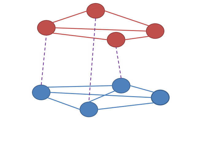
Figure 1: Demonstration of an interdependent network with coupling $q=0.75$ with dependency links shown as dashed lines. The $2$-core and $3$-core are the highest possible $k$-core in the top and bottom layers respectively, while still preserving all the dependency links.

At the steady state of the cascade process the network becomes fragmented into clusters of various sizes. Only the largest cluster (the “giant component”) is considered functional in this study and is the quantity of interest. The fraction of nodes $\phi^{\prime}_{\infty}$ remaining in the steady state is identical in both networks as the entire process is symmetrical for both networks and can be calculated using the formalism developed by Parshani et al Parshani et al. (2010),

$$\phi^{\prime}_{\infty}\equiv p_{0}[1-q(1-p_{0}M_{k_{a},r}(\phi^{\prime}_{\infty}))],$$ (1)

where $M_{k_{a},r}(p)$ is the fraction of nodes belonging to the giant component in a single network with a fraction $p$ of nodes occupied. The size of the giant component in the coupled networks at the steady state $\phi_{\infty}$ is

$$\phi_{\infty}=\phi^{\prime}_{\infty}M_{k_{a},r}(\phi^{\prime}_{\infty}).$$ (2)

The $k$-core formalism for single networks Baxter et al. (2011), based on local tree-like structure, gives the size of the giant component, rCl M_k_a,r(p) &= (1-r)∑_j=k_a^∞ P(j) Φ_j^k_a(X(p),Z(p)) +
r∑_j=k_a+1^∞ P(j) Φ_j^k_a+1(X(p),Z(p)), where

$$\Phi_{j}^{k}(X,Z)=\sum_{l=k}^{j}{j\choose l}(1-X)^{j-l}\sum_{m=1}^{l}{l\choose m}Z^{m}(X-Z)^{l-m}.$$

Here $Z$ and $X$ are the probabilities that, starting from any random link and node, respectively, the giant component will be reached. These are calculated using the self-consistent equations rCl Xfka,r(X,X) = Zfka,r(X,Z) = p, where rCl f_k_a,r(X,Z) &= (1-r) ∑_j=k_a^∞ jP(j)⟨j ⟩ Φ_j-1^k_a-1(X,Z) +
r ∑_j=k_a+1^∞ jP(j)⟨j ⟩ Φ_j-1^k_a(X,Z). The probabilities $X$ and $Z$ are equal when the local thresholds of $k$-core percolation are $k_{a}\geq 2$ Cellai et al. (2011). Equations (1) and (1)–(1) can be further simplified,

$$p_{0}=\frac{q-1+\sqrt{(q-1)^{2}+4q\frac{ZM_{k_{a},r}(X(Z),Z)}{f_{k_{a},r}(Z,Z)}}}{2qM_{k_{a},r}(X(Z),Z)}\equiv h_{k,q}(Z),$$ (3)

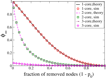
Figure S1: Comparison between theory and simulation of $k$-core percolation in two interdependent Scale-free networks with exponent $\gamma=2.5$, with both layers having identical local thresholds $k=1,2,3$. Simulation results were obtained for a system with $N=10^{6}$ nodes in each network. The minimum and maximum degree for nodes in each network were set to be $i_{min}=2$ and $i_{max}=1000$, respectively.

which can be used to solve for the probabilities $X$, $Z$ for any initial percolation probability $p_{0}$. The size of the giant component as a function of $p_{0}$, found by numerically solving Eqs. (2)–(1) and (3), is in excellent agreement with simulation results for both Erdős-Rényi (see Fig. 2) and scale-free networks (see Fig. S1 in the Supplementary Material).

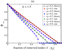
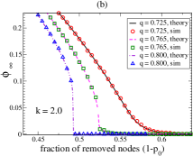
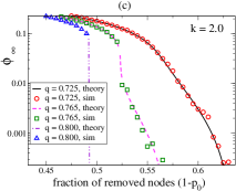
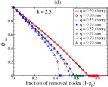
Figure 2: Comparison of theory (lines) and simulation (symbols) for two coupled Erdős-Rényi networks at fixed average local threshold a) $k=1.5$ b) $k=2.0$ c) $k=2.0$ (on a semi-log plot) and d) $k=2.5$. As the coupling $q$ is increased, $k$-core percolation transition changes from second-order to first-order. For $k=2.0$, a novel two-stage transition is seen at intermediate couplings. Simulation results agree well with the theory (more evident in the semi-log plot of panel (c)). Plots of comparison for more parameter values are given in the Supplementary Material (Fig. S2).

The function $h_{k,q}(Z)$ in Eq. (3) determines the nature of the phase transition and the critical percolation thresholds $p_{c}$, illustrated below in the example of two Erdős-Rényi networks.

To demonstrate the richness of the model that combines $k$-core and interdependency, we focus on two interdependent Erdős-Rényi networks. Both networks have identical degree distributions given by $P(i)=z_{1}^{i}\exp(-z_{1})/i!$ with the same average degree $z_{1}$. The function $f_{k_{a},r}$ is given by $f_{1,r}(X,Z)=1-e^{-z_{1}Z}$, $f_{1,r}(X,X)=1-re^{-z_{1}X}$ and since $X=Z$ for $k_{a}\geq 2$, $f_{2,r}(Z,Z)=1-e^{-z_{1}Z}(1+rz_{1}Z)$. The functions $M_{k_{a},r}$ are given by $M_{1,r}(X,Z)=1-e^{-z_{1}Z}-rz_{1}Ze^{-z_{1}X}$ and $M_{2,r}(Z)=1-(1-r)\frac{\Gamma(2,z_{1}Z)}{\Gamma(2)}-r\frac{\Gamma(3,z_{1}Z)}{\Gamma(3)}$, where $\Gamma(m,x)$ and $\Gamma(m)$ are incomplete and complete gamma functions, respectively, of order $m$.

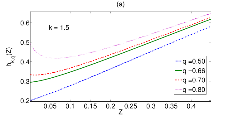
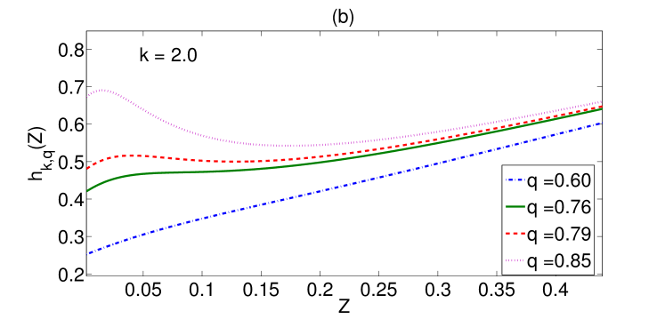
Figure S3: Comparison of behavior of the function $h_{k,q}(Z)$ for two coupled Erdős-Rényi networks at fixed average local threshold a) $k=1.5$ and b) $k=2.0$ at different couplings. As seen in the phase diagram (See Fig.S6), $k$-core percolation changes from a second-order at low couplings to a first-order at high couplings $q$ passing through a tricritical point for $k=1.5$, and through a two-stage transition for $k=2.0$. In both cases, $h_{k,q}(Z)$ is characterized by monotonically increasing behaviour corresponding to second-order transition and, by the presence of a global minima corresponding to first-order transition. For $k=1.5$, the inflection point occurs at $Z=0$, which immediately turns into a global minima as the coupling is increased, leading to a tricritical point. For $k=2.0$, the inflection point occurs at $Z>0$, which turns into a local minima followed by being a global minima as the coupling is increased, leading to a two-stage transition.

The behavior of the function $h_{k,q}(Z)$, Eq. (3), for fixed values of parameters as a function of $Z$ determines the nature of the $k$-core percolation transition. In general, the function $h_{k,q}(Z)$ has either (i) a monotonically increasing behavior, (ii) a local minimum, or (iii) a global minimum (see Fig. S3 in the Supplementary Material). Monotonically increasing behavior corresponds to a second-order percolation transition. When $h_{k,q}(Z)$ has a global minima, percolation transition is an abrupt (first-order) transition. The presence of local minima indicates that the percolation transition is a two-stage transition in which the giant component undergoes an abrupt (first-order) jump followed by a continuous transition as the occupation probability $p_{0}$ is decreased [see the case of $q=0.765$ in Fig. 2(c)]. Using this analysis, we plot the complete phase diagram of $k$-core percolation transition for Erdős-Rényi networks in Fig. 3.

The boundaries of the phase diagram (Fig. 3), $q=0$ and $k=1$ lines correspond to the cases of $k$-core percolation in single network and regular percolation in interdependent networks, respectively. We describe the complex nature of the combined $k$-core percolation and interdependent network model at intermediate couplings $0<q<1$, and contrast it with the known results at the boundaries. Parshani et al. Parshani et al. (2010) demonstrated that regular percolation in coupled networks changes from a second-order to first-order when it passes through a tricritical point at the critical coupling $q_{\rm tri,1}$. The tricritical nature is preserved in $k$-core percolation as the average local threshold $k$ is increased, but the tricritical coupling $q_{{\rm tri},k}$ increases with $k$, as can be seen in Fig. 3. The dependence of $q_{{\rm tri},k}$ on the average degree $z_{1}$ is

$$q_{{\rm tri},k}=1+X_{k-1,0}-\sqrt{(1+X_{k-1,0})^{2}-1},$$ (4)

where $X_{k-1,0}$ is the numerical solution for $X$ in self-consistent Eq. (1) when $Z=0$.

A first-order transition indicates network instability. Because instability increases with an increase in both the coupling $q$ and the average local threshold $k$—more nodes are removed during $k$-core percolation at higher local thresholds—we expect the $k$-core percolation transition to become first-order at lower couplings when the average local threshold is higher. Counterintuitively, Figure 3 shows that the tricritical coupling $q_{{\rm tri},k}$ increases with $k$. To test this further, we analyse Eq. (4). A perturbative expansion shows that $q_{{\rm tri},k}$ indeed increases with $k$, around $k=1$, as

$$q_{{\rm tri},k}=q_{\rm tri,1}+\frac{(k-1)e^{-1}+(k-1)^{2}e^{-2}}{z_{1}}\left(\frac{z_{1}+1}{\sqrt{2z_{1}+1}}-1\right),$$ (5)

where the tricritical coupling $q_{\rm tri,1}$ (consistent with results found in Ref. Gao et al. (2012b)) is given by

$$q_{\rm tri,1}=1+\frac{1}{z_{1}}-\sqrt{(1+\frac{1}{z_{1}})^{2}-1}.$$ (6)

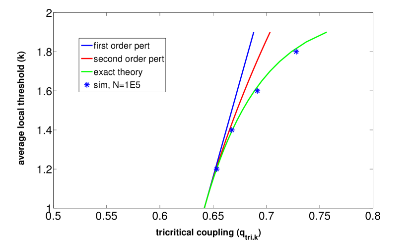
Figure S4: Plot of tricritical coupling $q_{{\rm tri},k}$ as a function of average threshold $k$ obtained from the numerical solution of perturbative expansion to first order, second order and exact equation given in the Eqs. (4, 5) in the main text. The numerical results are in excellent agreement with the simulation results (shown as symbols) for a network with $10^{5}$ nodes .

We compare the perturbative solution of Eq. (5) with the numerical solution of Eq. (4) and the simulation results in Fig. S4 (see Supplementary Material).

Above an average local threshold $k\lesssim 2$, the tricritical nature ceases to exist. Instead, as the coupling $q$ is increased, the $k$-core percolation transition goes through a two-stage transition as it changes from second-order to first-order. Figure 2(c) shows that this two-stage transition has characteristics of both first- and second-order transitions. The critical couplings that separate the two-stage transition from the first-order and second-order transition regions are $q_{c,1}$ and $q_{c,2}$, respectively. At the critical line $q_{c,2}(k)$, the function $h_{k,q}(Z)$ develops an inflection point at $Z>0$ that signals the development of a local minimum for $q>q_{c,2}$ (see Fig. S3(b) in the Supplementary Material). The condition for $q_{c,2}$ at a fixed $k$ is

$$h^{\prime}_{k,q_{c,2}}(Z_{0})=0\quad\&\quad h^{\prime\prime}_{k,q_{c,2}}(Z_{0})=0,$$ (7)

where the derivatives are taken with respect to $Z$ and the inflection point $Z_{0}$ must be determined using the relationship in Eq. (7). For couplings $q\leq q_{c,1}$, the global minimum of $h_{k,q}(Z)$ occurs at $Z=0$. For $q>q_{c,1}$, the global minimum shifts to $Z_{0}>0$. At the critical line $q_{c,1}(k)$, the function has global minima at both $Z=0$ and $Z_{0}>0$ (see Fig. S3(b) in the Supplementary Material) and this yields the conditions for the critical coupling $q_{c,1}$,

$$h_{k,q_{c,1}}^{\prime}(Z_{0})=0\quad\&\quad h_{k,q_{c,1}}(Z_{0})=h_{k,q_{c,1}}(Z=0).$$ (8)

In single networks, the k-core percolation transition reaches a tricritical point when the average local threshold is increased from $2$ to $3$ at $k_{c}=2.5$ Cellai et al. (2011). Figure 3 shows that this tricritical point is preserved when the coupling between the networks is increased up to a critical coupling $q_{c,2.5}$ and forms a second tricritical line. The point $q_{c,2.5}$ (point “X”) is a triple point surrounded by three phases. This critical coupling depends on the average degree $z_{1}$,

$$q_{c,2.5}=1+\frac{3}{2z_{1}}-\sqrt{(1+\frac{3}{2z_{1}})^{2}-1}.$$ (9)

The critical lines $q_{c,1}(k)$ and $q_{c,2}(k)$ can be calculated perturbatively around the point $q_{c,2.5}$. Using the expansion of $h_{k,q}(Z)$ around $Z=0$ with the conditions in Eq.(7) and Eq.(8), we get a general equation

$$a_{m}(1-q)^{4}+b_{m}q(1-q)^{2}+c_{m}q^{2}=0,$$ (10)

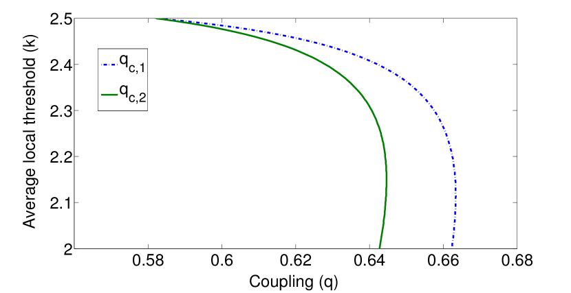
Figure S5: Numerical solution of the pertubrative expansion of $q_{c,1}(k)$ and $q_{c,2}(k)$ around the triple point $q_{c2,.5}$ given in Eq. (10) in the main text.

where $a_{m}=\frac{z_{1}^{2}}{36}(12(3-2m)\delta^{2}+6(m-2)\delta+1)$, $b_{m}=\frac{z_{1}}{6}(12(1-m)\delta^{2}+(4-2m)\delta-1),c_{m}=\delta^{2}+\delta+1/4$ with $\delta=2.5-k$. Solving Eq.(10) with $m=3$ and $m=4$ gives $q_{c,2}$ and $q_{c,1}$, respectively. The numerical solution of Eq. (10) are plotted in the Supplementary material (see Fig. S5).

Finally, for the average local threshold $2.5<k\leq 3$, $k$-core percolation transition remains first-order even when the coupling between the networks is increased.

The critical percolation thresholds and critical exponents for all three transitions discussed above can be calculated from the function $h_{k,q}(Z)$. At the second-order transition and the continuous part of the two-stage transition ($q<q_{c,1}$, the gray regions in Fig. 3), the critical behavior of the giant component takes the form $\phi_{\infty}\sim(p-p_{c,2})^{\beta_{2}}$, where $p_{c,2}=h_{k,q}(Z=0)$. The analytical expressions for $p_{c,2}$ are

$$p_{c,2}=\left\{\begin{array}[]{lcrcl}\frac{1}{z_{1}(1-q)},&1\leq k\leq 2&\\ \frac{1}{z_{1}(1-(k-2))(1-q)},&2\leq k\leq 2.5&\\ \end{array}\right.$$ (11)

We find the exponent $\beta_{2}$ by using the Taylor series expansion of the function $h_{k,q}(Z)$ around $Z=0$. The exponent depends on coupling, indicating that coupling changes the universality classes of these $k$-core percolation transitions. The exponents found at different points of the phase diagram are

$$\beta_{2}=\left\{\begin{array}[]{lcrcl}1,&1\leq k<2,q<q_{{\rm tri},k}&\\ 1/2,&1\leq k<2,q=q_{{\rm tri},k}&\\ 2,&2\leq k<2.5,q\leq q_{c,1}&\\ 1,&k=2.5,q<q_{c,2.5}&\\ 2/3,&k=2.5,q=q_{c,2.5}.&\end{array}\right.$$ (12)

At the first-order transition and the abrupt jump of the two-stage transition, the critical behavior of the giant component takes the form $\phi_{\infty}-\phi_{\infty,0}\sim(p-p_{c,1})^{\beta_{1}}$, where $p_{c,1}=h_{k,q}(Z_{0})$. $Z_{0}$ is the minimum of the function $h_{k,q}(Z)$ found using the condition $h_{k,q}^{\prime}(Z_{0})=0$. Both $p_{c,1}$ and $p_{c,2}$ are calculated numerically and are in good agreement with the simulations shown in Fig. 4. We calculate the critical exponent $\beta_{1}$ using a Taylor series expansion of the function $h_{k,q}(Z)$ around the minimum $Z_{0}$ and find that it is dependent only on coupling $q$

$$\beta_{1}=\left\{\begin{array}[]{lcrcl}1/3,&q=q_{c,2}&\\ 1/2,&q>q_{c,2}&.\end{array}\right.$$ (13)

The richness of the phase diagram is striking when the change in $k$-core percolation transition is considered as threshold $k$ is increased at fixed $q$. At certain fixed intermediate couplings, the $k$-core percolation transition changes from first-order $\rightarrow$ second-order $\rightarrow$ two-stage $\rightarrow$ first-order as the $k$-core threshold is increased (See vertical arrow in Fig. 3). Additionally, note that the result for fully interdependent networks $q=1$ is consistent with the result for the $k$-core percolation transition in multiplex networks in that they are both first-order for any average threshold $k$ Azimi-Tafreshi et al. (2014).

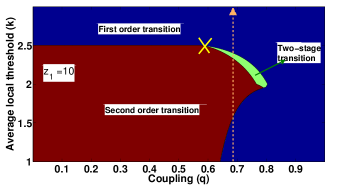
Figure 3: Complete phase diagram for $k$-core percolation transition for two interdependent Erdős-Rényi networks with average degree $z_{1}=10$ . Both networks have the same average local threshold per site $k=(1-r)k_{a}+r(k_{a}+1)$, with fraction $1-r$ of randomly chosen nodes having local threshold $k_{a}$ and the remaining nodes having local threshold $k_{a}+1$. Plots depicting the size of giant component as a function of removed nodes for different points in the phase diagram are given in Fig. 2 and Fig. S2 in the Supplementary Material. Symbol ’X’ in the phase diagram indicates the coupling $q_{c,2.5}$. The transition properties depend on the composition of the $k_{a}$-cores and not on average $k$. For example, the average local threshold of $3$ can be achieved by setting half of the nodes with local threshold $2$ and remaining nodes with local threshold $4$. $k$-core percolation of this heterogeneous case is found to be different from that of the homogeneous case where all the nodes have the same threshold $3$. Phase diagrams for different average degree $z_{1}$ are shown in the Supplementary Material (Fig. S6).

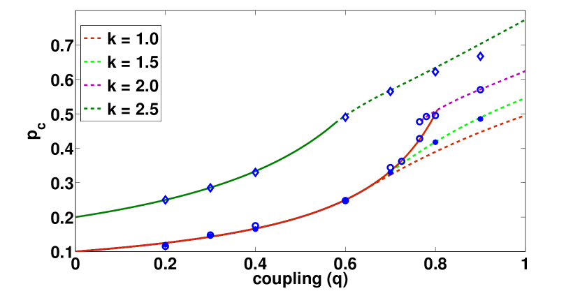
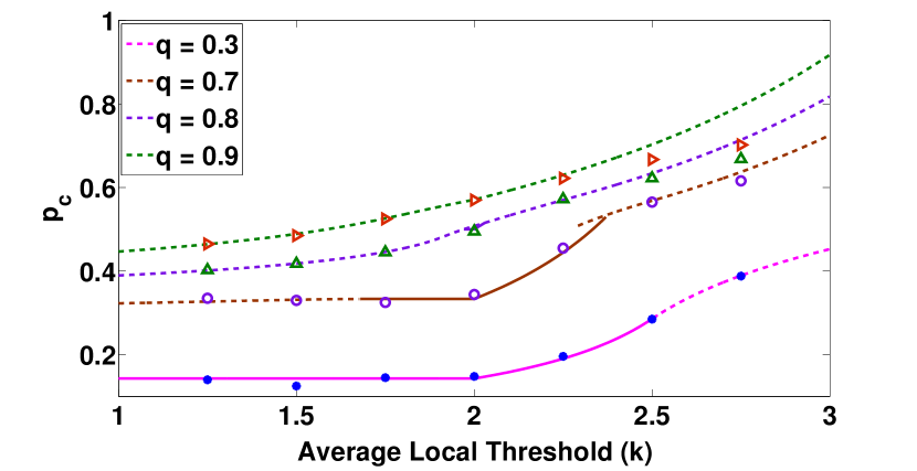
Figure 4: Percolation threshold $p_{c}$ as a function of (a) the coupling $q$ for fixed average local threshold $k=1.0,1.5,2.0,2.5$ representing horizontal lines in Fig. 3 (b) the average local threshold $k$ for several fixed coupling $q=0.3,0.7,0.8,0.9$ representing vertical lines in Fig. 3. Dashed and continuous lines indicate that the percolation threshold is at abrupt (first-order) jump and continuous transition respectively. Simulation results (shown as symbols) are obtained for a system with $10^{6}$ nodes in each network.

In conclusion, we have developed and analysed a general model that includes two realistic mechanisms: $k$-core percolation and interdependency between networks with any degree of coupling. We have verified our analytical solutions through extensive simulations. We have demonstrated the richness of combined effects through the complete phase diagram for $k$-core percolation transition in two interdependent Erdős-Rényi networks. The coupling between networks dramatically changes the critical behavior of $k$-core percolation found in single networks, and also yields new critical exponents that are calculated analytically. At fixed $k$-core threshold, the $k$-core percolation transition changes from second-order to first-order as the coupling is increased, either passing through a tricritical point or two-stage transition depending on the average local threshold. We calculated the tricritical couplings and phase boundaries of the two-stage transition shared with second and first-order transition regions. Counterintuitively, we find the tricritical coupling to increase with the $k$-core threshold. The richness of this generalized model is further emphasized with the $k$-core percolation transition, for certain fixed couplings, changing from first-order $\rightarrow$ second-order $\rightarrow$ two-stage $\rightarrow$ first-order as the $k$-core threshold is increased, in contrast to second-order $\rightarrow$ first-order for single networks. To test the universality of our results, we also analyzed, both analytically and numerically, the phase diagram for $k$-core percolation in interdependent random regular networks and found this system to be very similar to that of Erdős-Rényi networks (See Supplementary Material). Studying these new percolation transitions found in this generalized model will enable us to understand the importance and the rich effects of coupling between different resources in cascading failures that occur in real world systems, which will enable us to design more resilient systems.

Supplemental Material: $k$-core percolation in interdependent networks

I Comparison of Giant component from theory and simulations for two coupled scale-free networks

II Comparison of Giant component from theory and simulations for two coupled Erdős-Rényi networks

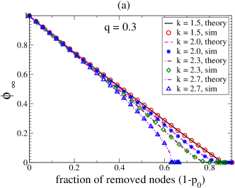
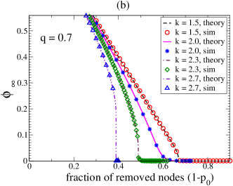
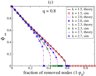
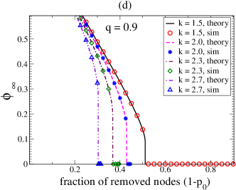
Figure S2: The giant component for two coupled Erdős-Rényi networks ($z_{1}=10$), computed numerically and through simulations, as a function of fraction of initially removed nodes $p_{0}$ at different average local threshold $k$ for couplings a) $q=0.3$ b) $q=0.7$ c) $q=0.8$ and d) $q=0.9$. For low coupling $q=0.3$, nature of $k$-core percolation is identical to that of single networks. For high couplings $q=0.8$ and $q=0.9$, $k$-core percolation is first-order indicating the increased instability of the system compared to single networks. For the intermediate coupling $q=0.7$, $k$-core percolation is initially first-order for $k=1.5$, which then becomes a continuous transition as the average local threshold is increased to $k=2.0$. The cascades during $k$-core percolation are expected to increase as the local threshold of nodes are increased, and therefore, $k$-core percolation would be (intuitively) expected to remain as first-order. As the average local threshold is increased further, the increased instability in the system is manifested into $k$-core percolation becoming a two-stage transition at $k=2.3$ and finally into a first-order transition for $k=2.7$. Simulation results (shown as symbols) are obtained for a system with $10^{6}$ nodes in each network.

III Comparison of behavior of the function $h_{k,q}(z)$ at tricritical point and two-stage transition

IV Plot of tricritical coupling as a function of average local threshold for $1<k<2$

V Perturbative solution for $q_{c,1}$ and $q_{c,2}$ around the triple point $q_{c,2.5}$

VI Phase diagram for two coupled Erdős-Rényi networks for different average degree $z1$

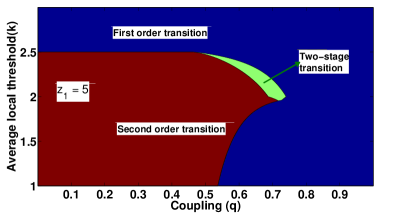
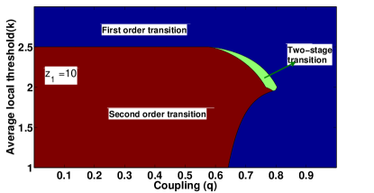
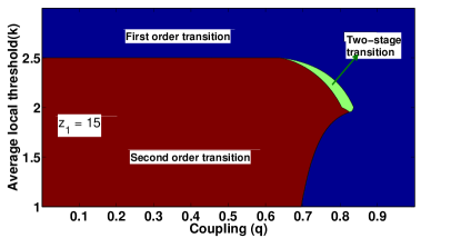
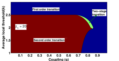
Figure S6: Complete phase diagram for $k$-core percolation transition for two coupled Erdős-Rényi networks with average degree $z_{1}=5,10,15,20$. Both the networks have the same average local threshold per site $k=(1-r)k_{a}+r(k_{a}+1)$, with fraction $1-r$ of nodes having local threshold $k_{a}$ and fraction $r$ of nodes having local threshold $k_{a}+1$. The transition properties depend on the composition of the $k_{a}$-cores and not on average threshold $k$. Width of the two-stage transition region in the phase diagram decreases as the average degree $z_{1}$ is increased.

VII Random regular network: Complete phase diagram

Consider two coupled Random Regular networks with identical degrees $z_{1}$. The function $f_{k_{a},r}$ is given by $f_{1,r}(X,Z)=1-(1-Z)^{z_{1}-1}$, $f_{1,r}(X,X)=1-r(1-X)^{z_{1}-1}$, and since $X=Z$ for $k_{a}\geq 2$, $f_{2,r}(Z,Z)=1-(1-Z)^{z_{1}-1}-rZ(z_{1}-1)(1-Z)^{z_{1}-2}$. The functions $M_{k_{a},r}$ are given by $M_{1,r}(X,Z)=1-(1-Z)^{z_{1}}-rz_{1}Z(1-X)^{z_{1}-1}$ and $M_{2,r}(Z)=1-(1-Z)^{z_{1}}-z_{1}Z(1-Z)^{z_{1}-1}-r\frac{z_{1}(z_{1}-1)}{2}Z^{2}(1-Z)^{z_{1}-2}$. Based on the behavior of $h_{k,q}(Z)$, the complete phase diagram for the percolation transition is plotted in Fig. S7. The features of the phase diagram are the same as those of coupled Erdős-Rényi networks, including identical critical exponents. The critical percolation thresholds are different and, for second-order and continuous part of the two-stage transitions for Random Regular networks is given by,

$$p_{c,2}=\left\{\begin{array}[]{lcrcl}\frac{1}{(z_{1}-1)(1-q)}\color[rgb]{0,0,0},&1\leq k\leq 2&\\ \frac{1}{(z_{1}-1)(1-(k-2))(1-q)},&2\leq k\leq 2.5&\\ \end{array}\right.$$ (S1)

The tricritical coupling for regular percolation in interdependent Random Regular networks depends on its degree $z_{1}$ as given in Eq. (S2).

$$q_{c,1}=1+\frac{z_{1}}{(z_{1}-1)(z_{1}-2)}-\sqrt{(1+\frac{z_{1}}{(z_{1}-1)(z_{1}-2)})^{2}-1}.$$ (S2)

The tricritical point found for average local threshold $k=2.5$ in single RR network is preserved in coupled networks as well. The tricritical nature persists only up to a critical coupling $q_{c,2.5}$ and its dependence on the degree $z_{1}$ is given by Eq. (S3).

$$q_{c,2.5}=1+\frac{3z_{1}}{2(z_{1}-2)(z_{1}-3)}-\sqrt{(1+\frac{3z_{1}}{2(z_{1}-2)(z_{1}-3)})^{2}-1}.$$ (S3)

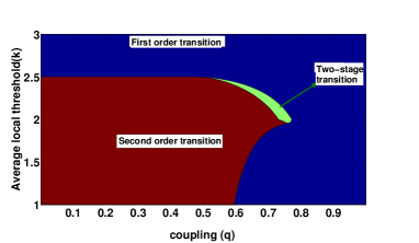
Figure S7: Complete phase diagram for $k$-core percolation transition for two coupled Random Regular networks with coupling $q$. Both the networks have the same local $k$-core threshold distribution. A fraction $r$ of randomly chosen nodes have local threshold $k_{a}+1$ and remaining nodes have $k_{a}$, resulting in average local threshold $k=(1-r)k_{a}+r(k_{a}+1)$. The phase diagram has similar features that were seen in two coupled Erdős-Rényi networks(Fig. S6). The critical exponents for all the regions in the phase diagram are identical to that of Erdős-Rényi networks as reported in the main text. The expressions for critical percolation thresholds for continuous transition part of both second-order and two-stage transitions are given in Eq. (S1).