Scalable Underapproximation for the Stochastic Reach-Avoid Problem for High-Dimensional LTI Systems using Fourier Transforms

Abstract

We present a scalable underapproximation of the terminal hitting time stochastic reach-avoid probability at a given initial condition, for verification of high-dimensional stochastic LTI systems. While several approximation techniques have been proposed to alleviate the curse of dimensionality associated with dynamic programming, these techniques are limited and cannot handle larger, more realistic systems. We present a scalable method that uses Fourier transforms to compute an underapproximation of the reach-avoid probability for systems with disturbances with arbitrary probability densities. We characterize sufficient conditions for Borel-measurability of the value functions. We exploit fixed control sequences parameterized by the initial condition (an open-loop control policy) to generate the underapproximation. For Gaussian disturbances, the underapproximation can be obtained using existing efficient algorithms by solving a convex optimization problem. Our approach produces non-trivial lower bounds and is demonstrated on a chain of integrators with 40 states.

I Introduction

Reachability analysis of discrete-time stochastic dynamical systems is an established verification tool that provides probabilistic guarantees of safety or performance, and has been applied to problems in fishery management and mathematical finance [1], motion planning in robotics [2, 3, 4], spacecraft docking [5], and autonomous survelliance [6]. In [1], two classes of problems characterize verification over a finite horizon — first hitting time and terminal hitting time – and dynamic programming approaches are formulated to solve both (similarly to [7, 8]). We focus on the finite time horizon terminal hitting time stochastic reach-avoid problem (referred to here as the terminal time problem for convenience), that is, computing the probability of hitting a target set at the terminal time, while avoiding an unsafe set during all the preceding time steps. Specifically, we construct an underapproximation to the terminal time problem from a known initial point, as opposed to the typical stochastic reach-avoid problem. This could be used as a query, for example, in evaluating feasibility of an initial trajectory an optimization problem.

The dynamic programming-based discretization approach (DPBDA), proposed in [8], approximately computes value functions for the terminal time problem, but relies on gridding, and hence suffers from the well-known curse of dimensionality. Attempts to circumvent this problem, via approximate dynamic programming [9, 10, 11], Gaussian mixtures [10], particle filters [11, 5], and convex chance-constrained optimization [5, 6], have been applied to systems that are at most 10-dimensional – far beyond the scope of what is possible with DPBDA, but not scalable to larger problems.

In this paper, we first characterize sufficient conditions for Borel-measurability of the value functions for the terminal time problem (characterized so far only for the first hitting time problem [12]). Using conditional expectations, we then establish that an open-loop formulation provides an underapproximation of the stochastic reach-avoid probability for linear systems [5]. We propose a scalable Fourier transform-based underapproximation (FTBU), for the terminal time problem, exploiting our prior work on uncontrolled stochastic reachable sets [2]. For an arbitrary probability density, the FTBU solves an optimization problem with a multi-dimensional integration as the objective function. For Gaussian disturbances, the objective function can be computed efficiently via existing algorithms [13], and the optimization problem is log-concave. Our approach does not require gridding of state, input, or disturbance spaces, and has low memory requirements in contrast to DPBDA.

Our main contribution is twofold: 1) a Fourier transform-based underapproximation of the terminal hitting time stochastic reach-avoid probability from a known initial condition, based on open-loop control sequences, and 2) the underlying theory that enables us to exploit measurability and convexity properties to assure a computationally feasible approach. We extend our previous work on Fourier transform-based stochastic reachable sets for uncontrolled systems [2] to systems with control inputs, although here we do not seek to compute the stochastic reach-avoid set [14].

In Section II, we describe the terminal time problem, its open-loop approximation, and relevant properties from probability theory and Fourier analysis. Section III presents sufficient conditions for Borel-measurability, and establishes the underapproximation result linking the problems in [1] and [5]. Section IV presents the FTBU and specialized results for Gaussian disturbances. We demonstrate scalability in Section V, through application to a 40D chain of integrators. Section VI concludes the work.

II Preliminaries and Problem Formulation

We denote the Borel $\sigma$-algebra by $\mathscr{B}(\cdot)$, a discrete-time time interval by $\mathbb{N}_{[a,b]}$ for $a,b\in\mathbb{N}$ and $a\leq b$, which inclusively enumerates all integers in between $a$ and $b$, random vectors with bold case, and non-random vectors with an overline. The indicator function of a non-empty set $\mathcal{S}$ is denoted by $1_{\mathcal{S}}(\bar{y})$, such that $1_{\mathcal{S}}(\bar{y})=1$ if $\bar{y}\in\mathcal{S}$ and is zero otherwise. We denote the $p$-dimensional identity matrix by $I_{p}$, and the matrix with all entries as ones by $\bar{1}_{p\times q}\in\mathbb{R}^{p\times q}$.

II-A Probability theory

A random vector $\boldsymbol{y}$ is a measurable transformation defined in the probability space $(\Omega,\mathscr{Y},\mathbb{P})$ with sample space $\Omega$, $\sigma$-algebra $\mathscr{Y}$, and probability measure over $\mathscr{Y}$, $\mathbb{P}$. A sub-$\sigma$-algebra of $\mathscr{Y}$ is a $\sigma$-algebra whose members also belong to $\mathscr{Y}$. The minimal $\sigma$-algebra of $\boldsymbol{y}$, the smallest sub-$\sigma$-algebra of $\mathscr{Y}$ over which $\boldsymbol{y}$ is measurable, is denoted by $\sigma(\boldsymbol{y})\subset\mathscr{Y}$. We typically consider Borel-measurable random vectors, $\boldsymbol{y}:\mathbb{R}^{p}\rightarrow\mathbb{R}^{p}$ with $\Omega=\mathbb{R}^{p}$ and $\mathscr{Y}=\sigma(\boldsymbol{y})=\mathscr{B}(\mathbb{R}^{p})$. For $N\in\mathbb{N}$, a random process is a sequence of random vectors ${\{\boldsymbol{y}_{k}\}}_{k=0}^{N}$ where the random vectors $\boldsymbol{y}_{k}$ are defined in the probability space $(\Omega,\mathscr{Y},\mathbb{P})$. The random vector $\boldsymbol{Y}={[\boldsymbol{y}_{0}\ \boldsymbol{y}_{1}\ \ldots\ \boldsymbol{y}_{N}]}^{\top}$ is defined in the probability space $(\Omega^{N+1},\sigma(\bigtimes_{k=0}^{N}\mathscr{Y}_{k}),\mathbb{P}_{\boldsymbol{Y}})$, with $\mathbb{P}_{\boldsymbol{Y}}$ induced from $\mathbb{P}$. See [15, 16] for details.

Conditional expectations transforms random variable $\boldsymbol{p}$ in $(\Omega,\mathscr{P},\mathbb{P})$ whose mean exists ($|\mathbb{E}\left[\boldsymbol{p}\right]|\leq\infty$) to a sub-$\sigma$-algebra $\mathscr{Q}$, i.e, $\mathscr{Q}$ is a $\sigma$-algebra with all its members containing in $\mathscr{P}$. For a $\mathscr{Q}$-measurable random variable $\boldsymbol{q}$ such that $\int_{\mathcal{S}}\boldsymbol{p}d\mathbb{P}=\int_{\mathcal{S}}\boldsymbol{q}d\mathbb{P}$ for all $\mathcal{S}\in\mathscr{Q}$, $\boldsymbol{q}=\mathbb{E}\left[\boldsymbol{p}\middle|\mathscr{Q}\right]$ almost surely (a.s.) [16, Sec. 7.1, Thm. 1].

1. For $\mathscr{Y}$-measurable random variables $\boldsymbol{y}_{1},\boldsymbol{y}_{2}$ with finite means, a sub-$\sigma$-algebra $\mathscr{G}\subset\mathscr{Y}$, if $\boldsymbol{y}_{1}\leq\boldsymbol{y}_{2}$ a.s., then $\mathbb{E}\left[\boldsymbol{y}_{1}\middle|\mathscr{G}\right]\leq\mathbb{E}\left[\boldsymbol{y}_{2}\middle|\mathscr{G}\right]$ a.s.  [16, Sec. 7.1, eq. (14, i and iii)].

2. For bounded random variables $\boldsymbol{y},\boldsymbol{z}$ that are $\mathscr{Y},\mathscr{Z}$-measurable respectively, if $|\mathbb{E}\left[\boldsymbol{y}\boldsymbol{z}\right]|\leq\infty$, then $\boldsymbol{y}\mathbb{E}\left[\boldsymbol{z}\middle|\mathscr{Y}\right]=\mathbb{E}\left[\boldsymbol{y}\boldsymbol{z}\middle|\mathscr{Y}\right]$ a.s. [16, Sec. 7.1, Thm. 3].

3. $\mathbb{E}\left[\mathbb{E}\left[\boldsymbol{y}\middle|\mathscr{G}_{2}\right]\middle|\mathscr{G}_{1}\right]=\mathbb{E}\left[\boldsymbol{y}\middle|\mathscr{G}_{1}\right]$ a.s. if $\mathscr{G}_{1}\subset\mathscr{G}_{2}\subset\sigma(\boldsymbol{y})$ and $\mathbb{E}\left[\boldsymbol{y}\right]\leq\infty$ [16, Sec. 7.1, eq. (14, v)].

The characteristic function (CF) of a random vector $\boldsymbol{y}\in\mathbb{R}^{p}$ with probability density function (PDF) $\psi_{\boldsymbol{y}}(\bar{z})$ is

$$\Psi_{\boldsymbol{y}}(\bar{\alpha}) \triangleq\mathbb{E}_{\boldsymbol{y}}\left[\mathrm{exp}\left({j\bar{\alpha}^{\top}\boldsymbol{y}}\right)\right]$$

$$=\int_{\mathbb{R}^{p}}e^{j\bar{\alpha}^{\top}\bar{z}}\psi_{\boldsymbol{y}}(\bar{z})d\bar{z}=\mathscr{F}\left\{\psi_{\boldsymbol{y}}(\cdot)\right\}(-\bar{\alpha})$$ (1)

where $\mathscr{F}\{\cdot\}$ denotes the Fourier transformation operator and $\bar{\alpha}\in\mathbb{R}^{p}$. Given a CF $\Psi_{\boldsymbol{y}}(\bar{\alpha})$, the PDF can be computed as

$$\psi_{\boldsymbol{y}}(\bar{z}) =\mathscr{F}^{-1}\left\{\Psi_{\boldsymbol{y}}(\cdot)\right\}(-\bar{z})$$

$$={\left(\frac{1}{2\pi}\right)}^{p}\int_{\mathbb{R}^{p}}e^{-j\bar{\alpha}^{\top}\bar{z}}\Psi_{\boldsymbol{y}}(\bar{\alpha})d\bar{\alpha}$$ (2)

where $\mathscr{F}^{-1}\{\cdot\}$ denotes the inverse Fourier transformation operator and $d\bar{\alpha}$ is short for $d\alpha_{1}d\alpha_{2}\ldots d\alpha_{p}$. Since PDFs are absolutely integrable, every PDF has a unique CF. See [17, Sec. 1], [18, Sec. 22.6], [15, Sec. 7.2, 8.2], [2, Sec. 2.1] for more details about CFs.

II-B Terminal stochastic reach-avoid analysis

Consider the discrete-time stochastic LTI system,

$$\boldsymbol{x}_{k+1} =A\boldsymbol{x}_{k}+B\bar{u}_{k}+\boldsymbol{w}_{k}$$ (3)

with state $\boldsymbol{x}_{k}\in\mathcal{X}=\mathbb{R}^{n}$, input $\bar{u}_{k}\in\mathcal{U}\subseteq\mathbb{R}^{m}$, disturbance $\boldsymbol{w}_{k}\in\mathcal{W}\subseteq\mathbb{R}^{n}$, and matrices $A,B$ assumed to be of appropriate dimensions. We assume that $\mathcal{U}$ is compact, $\boldsymbol{w}_{k}$ is absolutely continuous with a known PDF $\psi_{\boldsymbol{w}}$, and the random process $\boldsymbol{w}[\cdot]$ is independent and identical distributed (IID). Let $N$ be a finite time horizon. For any given sequence of (non-random) inputs $\bar{u}[\cdot]$ and an initial condition $\bar{x}_{0}\in\mathcal{X}$, the state $\boldsymbol{x}_{k}$ is a random vector for all $k\in\mathbb{N}_{[1,N]}$ via (3).

The system (3) can be equivalently described by a Markov control process with stochastic kernel that is a Borel-measurable function $Q:\mathscr{B}(\mathcal{X})\times\mathcal{X}\times\mathcal{U}\rightarrow[0,1]$, which assigns to each $\bar{x}\in\mathcal{X}$ and $\bar{u}\in\mathcal{U}$ a probability measure on the Borel space $(\mathcal{X},\mathscr{B}(\mathcal{X}))$. For (3),

$$Q(d\bar{y}|\bar{x},\bar{u}) =\psi_{\boldsymbol{w}}(\bar{y}-A\bar{x}-B\bar{u})d\bar{y}.$$ (4)

We define a Markov policy $\pi=(\mu_{0},\mu_{1},\ldots,\mu_{N-1})\in\mathcal{M}$ as a sequence of universally measurable maps $\mu[\cdot]:\mathcal{X}\rightarrow\mathcal{U}$. The random vector $\boldsymbol{X}=[\boldsymbol{x}^{\top}_{1}\ \boldsymbol{x}^{\top}_{2}\ \ldots\ \boldsymbol{x}^{\top}_{N}]^{\top}$, defined in $(\mathcal{X}^{N},\mathscr{B}(\mathcal{X}^{N}),\mathbb{P}_{\boldsymbol{X}}^{\bar{x}_{0},\pi})$ [1], has probability measure $\mathbb{P}_{\boldsymbol{X}}^{\bar{x}_{0},\pi}$ defined using $Q$ [19, Prop. 7.45].

Let $\mathcal{S},\mathcal{T}\in\mathscr{B}(\mathcal{X})$. Define the terminal time probability, $\hat{r}_{\bar{x}_{0}}^{\pi}(\mathcal{S},\mathcal{T})$, for known $\bar{x}_{0}$ and $\pi$, as the probability that the execution with policy $\pi$ is inside the target set $\mathcal{T}$ at time $N$ and stays within the safe set $\mathcal{S}$ for all time up to $N$. From [1],

$$\hat{r}_{\bar{x}_{0}}^{\pi}(\mathcal{S},\mathcal{T}) =\mathbb{P}_{\boldsymbol{X}}^{\bar{x}_{0},\pi}\left\{\boldsymbol{x}_{N}\in\mathcal{T}\wedge\boldsymbol{x}_{k}\in\mathcal{S}\ \forall k\in\mathbb{N}_{[0,N-1]}\right\}.$$

From [1, Def. 10], a Markov policy $\pi^{\ast}$ is a maximal reach-avoid policy in the terminal sense if and only if it is the optimal solution of Problem A, defined as

$$\begin{array}[]{rl}\mbox{A}:&\hat{r}_{\bar{x}_{0}}^{\pi^{\ast}}(\mathcal{S},\mathcal{T})=\sup_{\pi\in\mathcal{M}}\hat{r}_{\bar{x}_{0}}^{\pi}(\mathcal{S},\mathcal{T})\end{array}$$ (6)

The solution of Problem A is characterized via dynamic programming [1, Thm. 11]. Define $\hat{V}_{k}^{\ast}:\mathcal{X}\rightarrow[0,1],\ k\in\mathbb{N}_{[0,N]}$, by the backward recursion for $\bar{x}\in\mathcal{X}$,

$$\hat{V}_{N}^{\ast}(\bar{x}) =1_{\mathcal{T}}(\bar{x})$$ (7)

$$\hat{V}_{k}^{\ast}(\bar{x}) =\sup_{\bar{u}\in\mathcal{U}}1_{\mathcal{S}}(\bar{x})\int_{\mathcal{X}}\hat{V}_{k+1}^{\ast}(\bar{y})Q(d\bar{y}|\bar{x},\bar{u}).$$ (8)

Then, the optimal value to Problem A is $\hat{r}_{\bar{x}_{0}}^{\pi^{\ast}}(\mathcal{S},\mathcal{T})=\hat{V}_{0}^{\ast}(\bar{x}_{0})$ for every $\bar{x}_{0}\in\mathcal{X}$.

Lemma 1.

[1, Thm. 11] A sufficient condition for existence of a maximal Markov policy for Problem A is

$$\mathcal{U}_{k}(\bar{x},\lambda) =\{\bar{u}\in\mathcal{U}:\int_{\mathcal{X}}\hat{V}_{k+1}^{\ast}(\bar{y})Q(\bar{y}|\bar{x},\bar{u})d\bar{y}\geq\lambda\}$$ (9)

and $\mathcal{U}_{k}$ is compact for all $\lambda\in\mathbb{R},\bar{x}\in\mathcal{X}$ and $k\in\mathbb{N}_{[0,N-1]}$.

Lemma 1 assures universal measurability of $\hat{V}_{k}^{\ast}(\cdot)$, and that the Markov policy $\pi^{\ast}$ consists of universally measurable maps $\mu^{\ast}_{k}$  [7, Thm. 1 proof]. However, evaluating (9) is difficult. We propose alternative sufficient conditions, which are easier to evaluate, and guarantee Borel-measurability (stronger than universal measurability [19, Defn. 7.20]).

II-C Open-loop stochastic reach-avoid analysis

With $\bar{U}=[\bar{u}^{\top}_{0}\ \bar{u}^{\top}_{1}\ \ldots\ \bar{u}^{\top}_{N-1}]^{\top}\in\mathcal{U}^{N}$ and $\boldsymbol{W}=[\boldsymbol{w}^{\top}_{0}\ \boldsymbol{w}^{\top}_{1}\ \ldots\ \boldsymbol{w}^{\top}_{N-1}]^{\top}\in\mathcal{W}^{N}$, we obtain

$$\boldsymbol{X} =\bar{A}\bar{x}_{0}+\bar{H}\bar{U}+\bar{G}\boldsymbol{W}.$$ (10)

The matrices $\bar{A},\bar{H},\bar{G}$ are given by specific combinations of the matrices $A$ and $B$ (see [20, Sec. 2]).

Consider an open-loop policy $\rho:\mathcal{X}\rightarrow\mathcal{U}^{N}$ which provides an open-loop sequence of inputs $\rho(\bar{x}_{0})$ for every initial condition $\bar{x}_{0}$. Then $\boldsymbol{X}$, defined in (10) under the action of $\rho(\bar{x}_{0})$, lies in the probability space $(\mathcal{X}^{N},\mathscr{B}(\mathcal{X}^{N}),\mathbb{P}_{\boldsymbol{X}}^{\bar{x}_{0},\rho(\bar{x}_{0})})$, with $\mathbb{P}_{\boldsymbol{X}}^{\bar{x}_{0},\rho(\bar{x}_{0})}$ defined using $Q$ [19, Prop. 7.45]. Note that $\rho(\bar{x}_{0})\not\in\mathcal{M}$, since universally measurable maps $\mu_{k}(\cdot)$ are functions of $\boldsymbol{x}_{k}$, not $\bar{x}_{0}$. Consequently, a Markov policy with $\mu_{k}(\cdot)$ as constants is a special case of $\rho(\cdot)$.

In [5], the authors approximate Problem A, without establishing the direction of approximation, with Problem B,

$$\begin{array}[]{rl}\mbox{B:}&\begin{array}[]{rcl}\mbox{maximize}&&\hat{r}_{\bar{x}_{0}}^{\rho(\bar{x}_{0})}(\mathcal{S},\mathcal{T})\\ \mbox{subject to}&&\left\{\begin{array}[]{rl}\boldsymbol{X}&\sim\mathbb{P}_{\boldsymbol{X}}^{\bar{x}_{0},\rho(\bar{x}_{0})}\\ \rho(\bar{x}_{0})&\in\mathcal{U}^{N}\\ \end{array}\right.\end{array}\end{array}$$ (16)

with decision variable $\rho(\bar{x}_{0})$, and

$$\hat{r}_{\bar{x}_{0}}^{\rho(\bar{x}_{0})}(\mathcal{S},\mathcal{T}) =\mathbb{P}_{\boldsymbol{X}}^{\bar{x}_{0},\rho(\bar{x}_{0})}\left\{\boldsymbol{x}_{N}\in\mathcal{T}\wedge\boldsymbol{x}_{k}\in\mathcal{S}\ \forall k\in\mathbb{N}_{[0,N-1]}\right\}.$$

The optimal solution to Problem B is $\rho^{\ast}(\bar{x}_{0})$. Since $\rho(\bar{x}_{0})\not\in\mathcal{M}$, the relation between Problems A and B, apart from structural similarity, is not evident. Problem B was solved in [5] approximately via particle filter and chance-constrained optimization methods.

We first demonstrate that Problem B underapproximates Problem A, then use a Fourier transform-based approach that enables an exact solution to Problem B.

Problem 1.

Characterize the sufficient conditions under which $\hat{V}_{k}^{\ast}(\cdot)$ and $\mu_{k}^{\ast}(\cdot)$ are Borel-measurable for the terminal time problem.

Problem 2.

Show that the terminal time problem (Problem A) is underapproximated by the open-loop formulation (Problem B).

Problem 3.

a) Construct a scalable method for solving Problem B by characterizing the forward stochastic reach probability density for stochastic linear systems controlled by $\rho(\cdot)$ when $\boldsymbol{w}$ has an arbitrary PDF. Additionally, b) formulate Problem B as a convex optimization problem when $\boldsymbol{w}$ is Gaussian.

III Theoretical results

III-A Sufficient conditions for Borel-measurability of $\hat{V}_{k}^{\ast}(\cdot)$

Definition 1.

[19, Defn. 7.12] A stochastic kernel $Q(\cdot|\bar{x},\bar{u})$ is continuous if for every $(\bar{x},\bar{u})\in\mathcal{X}\times\mathcal{U}$ and every sequence $(\bar{x}_{i},\bar{u}_{i})\xrightarrow{i\rightarrow\infty}(\bar{x},\bar{u})$,

$$\lim_{i\rightarrow\infty}Q(d\bar{y}|(\bar{x}_{i},\bar{u}_{i})) =Q(d\bar{y}|(\bar{x},\bar{u})).$$ (17)

Lemma 2.

If the PDF of the disturbance $\boldsymbol{w}$ $\psi_{\boldsymbol{w}}$ is continuous, then $Q(\cdot|\bar{x},\bar{u})$ defined in (4) is continuous.

Lemma 2 follows from the fact that continuity is preserved by composition [21, Cor. 13.1.7]. We have the following theorem, similar to [12, Prop. 3].

Theorem 1.

If $\mathcal{U}$ is compact and $Q(\cdot|\bar{x},\bar{u})$ is continuous, then $\hat{V}_{k}^{\ast}(\cdot)$ are Borel-measurable functions for $k\in\mathbb{N}_{[0,N]}$ and $\pi^{\ast}$, comprised of Borel-measurable maps $\mu_{k}^{\ast}(\cdot)$, exists.

Proof: (By induction) Since $\mathcal{S},\mathcal{T}$ are Borel sets, $1_{\mathcal{S}}(\cdot)$ and $1_{\mathcal{T}}(\cdot)$ are Borel-measurable functions, and the result for $k=N$ follows trivially. Consider the base case $k=N-1$. Since $\hat{V}_{N}^{\ast}(\cdot)$ is a bounded Borel-measurable function and $Q(\cdot|\bar{x},\bar{u})$ is a Borel-measurable function, continuous over $\mathcal{X}\times\mathcal{U}$, $\int_{\mathcal{X}}\hat{V}_{N}^{\ast}(\bar{y})Q(d\bar{y}|\bar{x},\bar{u})$ is continuous over $\mathcal{X}\times\mathcal{U}$ [22, Fact 3.9]. Since continuity implies upper semi-continuity [19, Lem. 7.13 (b)] and Borel-measurablity [16, Sec. 1.4], and $\mathcal{U}$ is compact, an optimal Borel-measurable input map $\mu_{N-1}^{\ast}(\cdot)$ exists and $\int_{\mathcal{X}}\hat{V}_{N}^{\ast}(\bar{y})Q(d\bar{y}|\bar{x},\mu_{N-1}^{\ast}(\bar{x}))$ is Borel-measurable over $\mathcal{X}$ [23, Thm. 2]. Finally, $\hat{V}^{\ast}_{N-1}(\cdot)$ is Borel-measurable since the product operator preserves Borel-measurability [21, Cor. 18.5.6]. For the case $k=t$, assume for induction that $\hat{V}_{t+1}^{\ast}(\cdot)$ is Borel-measurable. By the same arguments as above, a Borel-measurable $\mu_{t}^{\ast}(\cdot)$ exists and $\hat{V}_{t}^{\ast}(\cdot)$ is Borel-measurable, completing the proof.   

Theorem 1 addresses Problem 1. Since Borel-measurability implies universal measurability [19, Defn. 7.20], the hypotheses of Theorem 1 is stricter than Lemma 1, but can be easily checked, and implies that $\hat{V}_{k}^{\ast}(\boldsymbol{x}_{k})$ is a $\mathscr{B}([0,1])$-measurable random variable $\forall k\in\mathbb{N}_{[0,N]}$. The continuity requirements in Theorem 1 and Lemma 2 may be weakened to include exponential densities [19, Sec. 8.3].

III-B Problem B underapproximates Problem A

Next, we address Problem 2. For $\boldsymbol{x}_{k}=\bar{x}$, denote the expectation defined by $Q(\cdot|\bar{x},\bar{u})$ as $\mathbb{E}_{\boldsymbol{x}}^{\bar{u}}$. Under the conditions proposed by Theorem 1, we know that $\hat{V}_{k+1}^{\ast}(\boldsymbol{x}_{k+1})$ is a Borel-measurable random variable for all $k\in\mathbb{N}_{[0,N]}$. From (8), for any $k\in\mathbb{N}_{[0,N-1]}$, we have almost surely (a.s.)

$$\hat{V}_{k}^{\ast}(\bar{x}) =\sup_{\bar{u}\in\mathcal{U}}1_{\mathcal{S}}(\bar{x})\mathbb{E}_{\boldsymbol{x}}^{\bar{u}}\left[\hat{V}_{k+1}^{\ast}(\boldsymbol{x}_{k+1})\middle|\boldsymbol{x}_{k}=\bar{x}\right].$$ (18)

Using Theorem 1 and properties of conditional expectations, we can show the following theorem. See [24] for the proof.

Note that the state $\boldsymbol{x}_{k}$ is not an independent random vector, but part of a Markov control process controlled by a sequence of actions. Therefore, the conditional expectation in (18) is defined on the $\sigma$-algebra $\sigma(\overline{\boldsymbol{x}_{k}})=\sigma(\boldsymbol{x}_{0},\boldsymbol{x}_{1},\ldots,\boldsymbol{x}_{k})$. For any $k\in\mathbb{N}_{[0,N-1]}$, we have from (18)

$$\hat{V}_{k}^{\ast}(\boldsymbol{x}_{k}) =\sup_{\bar{u}\in\mathcal{U}}1_{\mathcal{S}}(\boldsymbol{x}_{k})\mathbb{E}_{\boldsymbol{x}}^{\bar{u}}\left[\hat{V}_{k+1}^{\ast}(\boldsymbol{x}_{k+1})\middle|\sigma(\overline{\boldsymbol{x}_{k}})\right]\mbox{a.s. }.$$ (19)

Also, by the definition of a stochastic process [16, Sec. 5.3],

$$\sigma(\overline{\boldsymbol{x}_{k}})\subset\sigma(\overline{\boldsymbol{x}_{k+1}})\ \forall k\in\mathbb{N}_{[0,N-1]}.$$ (20)

Theorem 2.

If $\mathcal{U}$ is compact and $Q(\cdot|\bar{x},\bar{u})$ is continuous, then $\hat{r}_{\bar{x}_{0}}^{\rho^{\ast}(\bar{x}_{0})}(\mathcal{S},\mathcal{T})\leq\hat{r}_{\bar{x}_{0}}^{\pi^{\ast}}(\mathcal{S},\mathcal{T})\mbox{ a.s. in }\bar{x}_{0}\in\mathcal{X}.$

Proof: For notational brevity, given $a\in\mathbb{N}_{[0,N]},\ b\in\mathbb{N}_{[0,N-1]}$, we define $U_{a}^{b}\stackrel{{\scriptstyle\triangle}}{{=}}(\bar{u}_{a},\bar{u}_{a+1},\ldots,\bar{u}_{b})$ for some $U\in\mathcal{U}^{N}$ with $U_{0}^{N-1}=U$ and $U_{N}^{N-1}$ as empty. We will later use a similar definition for $\boldsymbol{X}$.

For $k\in\mathbb{N}_{[0,N-1]}$, define $\hat{W}_{k}:\mathcal{X}\times\mathcal{U}^{N-k}\rightarrow[0,1]$ based on (18), (a.s.)

$$\hat{W}_{k}(\bar{x},U_{k}^{N-1}) \triangleq 1_{\mathcal{S}}(\bar{x})\mathbb{E}_{\boldsymbol{x}}^{\bar{u}_{k}}\left[\hat{W}_{k+1}(\boldsymbol{x}_{k+1},U_{k+1}^{N-1})\middle|\boldsymbol{x}_{k}=\bar{x}\right]$$

$$\hat{W}_{N}(\bar{x},U_{N}^{N-1}) \triangleq 1_{\mathcal{T}}(\bar{x}).$$

We see that $\hat{W}_{k}(\cdot)$ are Borel measurable by a straight-forward proof by induction. Next, we prove:

$$\begin{array}[]{ll}\mbox{S1:}&\hat{W}_{k}(\bar{x},U_{k}^{N-1})\leq\hat{V}_{k}^{\ast}(\bar{x})\mbox{ a.s. in }\bar{x}\in\mathcal{X},\forall k\in\mathbb{N}_{[0,N-1]}\\ \mbox{S2:}&\sup_{\rho(\bar{x}_{0})\in\mathcal{U}^{N}}\hat{W}_{0}(\bar{x}_{0},\rho(\bar{x}_{0}))=\hat{r}_{\bar{x}_{0}}^{\rho^{\ast}(\bar{x}_{0})}(\mathcal{S},\mathcal{T})\mbox{ a.s. in }\bar{x}_{0}.\end{array}$$

S1 implies $\sup_{\rho(\bar{x}_{0})\in\mathcal{U}^{N}}\hat{W}_{0}(\bar{x}_{0},\rho(\bar{x}_{0}))\leq\hat{V}_{0}^{\ast}(\bar{x}_{0})$ a.s. in $\bar{x}_{0}\in\mathcal{X}$. Thus, the proof is complete via S2 and the fact that $\hat{V}_{0}^{\ast}(\bar{x}_{0})=\hat{r}_{\bar{x}_{0}}^{\pi^{\ast}}(\mathcal{S},\mathcal{T})$ for every $\bar{x}_{0}\in\mathcal{X}$.

Proof of S1: (By induction) The base case is $k=N-1$. Since $U_{N-1}^{N-1}=\bar{u}_{N-1}$,

$$\hat{W}_{N-1}(\bar{x},\bar{u}_{N-1}) \triangleq 1_{\mathcal{S}}(\bar{x})\mathbb{E}_{\boldsymbol{x}}^{\bar{u}_{N-1}}\left[1_{\mathcal{T}}(\boldsymbol{x}_{N})\middle|\boldsymbol{x}_{N-1}=\bar{x}\right]\mbox{a.s. }.$$

From (18) and (7), we have (a.s.)

$$\hat{W}_{N-1}(\bar{x},\bar{u}_{N-1}) \leq\sup_{\bar{u}_{N-1}\in\mathcal{U}}\hat{W}_{N-1}(\bar{x},\bar{u}_{N-1})=\hat{V}_{N-1}^{\ast}(\bar{x}).$$

For the case $k=t$, assume for induction that $\hat{W}_{t+1}(\bar{x},U_{t+1}^{N-1})\leq\hat{V}_{t+1}^{\ast}(\bar{x})$ a.s. in $\bar{x}\in\mathcal{X}$. We have to show $\hat{W}_{t}(\bar{y},U_{t}^{N-1})\leq\hat{V}_{t}^{\ast}(\bar{y})$ a.s. in $\bar{y}\in\mathcal{X}$. By Property P1 and (19), we have (a.s.)

$$\hat{W}_{t}(\bar{y},U_{t}^{N-1}) \leq\sup_{\bar{u}_{t}\in\mathcal{U}}\hat{W}_{t}(\bar{y},U_{t}^{N-1})$$

$$\leq\sup_{\bar{u}_{t}\in\mathcal{U}}1_{\mathcal{S}}(\bar{y})\mathbb{E}_{\boldsymbol{x}}^{\bar{u}_{t}}\left[\hat{W}_{t+1}(\boldsymbol{x}_{t+1},U_{t+1}^{N-1})\middle|\boldsymbol{x}_{t}=\bar{y}\right]$$

$$\leq\sup_{\bar{u}_{t}\in\mathcal{U}}1_{\mathcal{S}}(\bar{y})\mathbb{E}_{\boldsymbol{x}}^{\bar{u}_{t}}\left[\hat{V}^{\ast}_{t+1}(\boldsymbol{x}_{t+1})\middle|\boldsymbol{x}_{t}=\bar{y}\right]$$

$$=\hat{V}_{t}^{\ast}(\bar{y}).$$

This completes the proof of S1.

Proof of S2: We use the definition of $\hat{W}_{k}(\cdot)$ based on $\sigma$-algebra (similar to (19)). By (20), $1_{\mathcal{S}}(\boldsymbol{x}_{k})$ is a $\sigma(\overline{\boldsymbol{x}_{t}})$-measurable random variable for $t\in\mathbb{N}_{[k,N]}$. Expanding $\hat{W}_{0}(\cdot)$ and $\hat{W}_{1}(\cdot)$ and using Property P2, we have (a.s.)

$$\hat{W}_{0}(\boldsymbol{x}_{0},U) =1_{\mathcal{S}}(\boldsymbol{x}_{0})\mathbb{E}_{\boldsymbol{x}}^{\bar{u}_{0}}\left[\hat{W}_{1}(\boldsymbol{x}_{1},U_{1}^{N-1})\middle|\sigma(\boldsymbol{x}_{0})\right]$$

$$=\mathbb{E}_{\boldsymbol{x}}^{\bar{u}_{0}}\left[1_{\mathcal{S}}(\boldsymbol{x}_{0})\hat{W}_{1}(\boldsymbol{x}_{1},U_{1}^{N-1})\middle|\sigma(\boldsymbol{x}_{0})\right]$$

$$=\mathbb{E}_{\boldsymbol{x}}^{\bar{u}_{0}}\Big{[}1_{\mathcal{S}}(\boldsymbol{x}_{0})1_{\mathcal{S}}(\boldsymbol{x}_{1})$$

$$\quad\quad\left.\mathbb{E}_{\boldsymbol{x}}^{\bar{u}_{1}}\left[\hat{W}_{2}(\boldsymbol{x}_{2},U_{2}^{N-1})\middle|\sigma(\overline{\boldsymbol{x}_{1}})\right]\middle|\sigma(\boldsymbol{x}_{0})\right]$$

$$=\mathbb{E}_{\boldsymbol{x}}^{\bar{u}_{0}}\Big{[}\mathbb{E}_{\boldsymbol{x}}^{\bar{u}_{1}}\Big{[}1_{\mathcal{S}}(\boldsymbol{x}_{0})1_{\mathcal{S}}(\boldsymbol{x}_{1})$$

$$\quad\quad\left.\left.\hat{W}_{2}(\boldsymbol{x}_{2},U_{2}^{N-1})\middle|\sigma(\overline{\boldsymbol{x}_{1}})\right]\middle|\sigma(\boldsymbol{x}_{0})\right]$$

From Property P3 and (20), we have (a.s.)

$$\hat{W}_{0}(\boldsymbol{x}_{0},U)=\mathbb{E}_{\boldsymbol{X}_{1}^{2}}^{U_{0}^{1}}\left[\left(\prod_{k=0}^{1}1_{\mathcal{S}}(\boldsymbol{x}_{k})\right)\hat{W}_{2}(\boldsymbol{x}_{2},U_{2}^{N-1})\middle|\sigma(\boldsymbol{x}_{0})\right]$$

We repeatedly expand $\hat{W}_{k}(\cdot)$ for $k\in\mathbb{N}_{[2,N]}$ and apply the arguments presented above to obtain

$$\hat{W}_{0}(\boldsymbol{x}_{0},U)=\mathbb{E}_{\boldsymbol{X}_{1}^{N}}^{U_{0}^{N-1}} \left[\left(\prod_{k=0}^{N-1}1_{\mathcal{S}}(\boldsymbol{x}_{k})\right)1_{\mathcal{T}}(\boldsymbol{x}_{N})\middle|\sigma(\boldsymbol{x}_{0})\right]\mbox{ a.s.}$$

By definition of $\mathbb{P}_{\boldsymbol{X}}^{\bar{x}_{0},\rho(\bar{x}_{0})}$, ($\boldsymbol{X}_{1}^{N}=\boldsymbol{X},U_{0}^{N-1}=U\triangleq\rho(\bar{x}_{0})$)

$$\hat{W}_{0}(\bar{x}_{0},\rho(\bar{x}_{0}))=\hat{r}_{\bar{x}_{0}}^{\rho(\bar{x}_{0})}(\mathcal{S},\mathcal{T})\mbox{ a.s.},$$

and the definition of $\rho^{\ast}(\bar{x}_{0})$ completes the proof of S2.   

We denote the optimal value of Problem B as $\hat{W}_{0}^{\ast}(\bar{x}_{0})$.

IV Under-approximation via Fourier transforms

IV-A FTBU using an analytical expression for $\hat{r}_{\bar{x}_{0}}^{\rho(\bar{x}_{0})}(\mathcal{S},\mathcal{T})$

Let the PDF of the random vector $\boldsymbol{X}$ parameterized by the initial condition $\bar{x}_{0}$ and the input vector $\bar{U}$ be $\psi_{\boldsymbol{X}}(\bar{X};\bar{x}_{0},\bar{U})$. The objective of Problem B $\hat{r}_{\bar{x}_{0}}^{\rho(\bar{x}_{0})}(\mathcal{S},\mathcal{T})$ is

$$\hat{r}_{\bar{x}_{0}}^{\rho(\bar{x}_{0})}(\mathcal{S},\mathcal{T}) =\int_{\mathcal{T}}\underbrace{\int_{\mathcal{S}}\ldots\int_{\mathcal{S}}}_{\text{$N-1$ times}}\psi_{\boldsymbol{X}}(\bar{X};\bar{x}_{0},\rho(\bar{x}_{0}))d\bar{X}$$ (21)

where $\bar{X}={[\bar{x}_{1}^{\top}\ \bar{x}_{2}^{\top}\ \ldots\ \bar{x}_{N}^{\top}]}^{\top}\in\mathcal{X}^{N}$, $\bar{x}_{k}\in\mathcal{X}\ \forall k\in\mathbb{N}_{[1,N]}$, and $d\bar{X}$ is short for $d\bar{x}_{1}d\bar{x}_{2}\ldots d\bar{x}_{N}$. Therefore, if $\psi_{\boldsymbol{X}}$ is known, then $\hat{r}_{\bar{x}_{0}}^{\rho(\bar{x}_{0})}(\mathcal{S},\mathcal{T})$ is a $nN$-dimensional integral of a PDF $\psi_{\boldsymbol{X}}$ over $\mathcal{S}\times\mathcal{S}\times\ldots\times\mathcal{T}$. Determining $\psi_{\boldsymbol{X}}$ for a known $\bar{U}$ can be posed as a forward stochastic reachability problem using the CF of $\boldsymbol{W}$ [2, Prop. P3] defined as

$$\Psi_{\boldsymbol{W}}(\bar{\alpha}) =\prod_{k=0}^{N-1}\Psi_{\boldsymbol{w}}(\bar{\alpha}_{k})$$ (22)

where $\bar{\alpha}={[\bar{\alpha}_{0}^{\top}\ \bar{\alpha}_{1}^{\top}\ \ldots\ \bar{\alpha}_{N-1}^{\top}]}^{\top}\in\mathbb{R}^{(nN)}$ and $\bar{\alpha}_{k}\in\mathbb{R}^{n}$ for all $k\in\mathbb{N}_{[0,N-1]}$. We compute $\psi_{\boldsymbol{X}}$ via Proposition 1.

Proposition 1.

For initial state $\bar{x}_{0}\in\mathcal{X}$, dynamics as in (10), and open-loop control vector $\bar{U}$, the PDF and CF of $\boldsymbol{X}$ are

$$\Psi_{\boldsymbol{X}}(\bar{\beta};\bar{x}_{0},\bar{U}) =\exp(j\bar{\beta}^{\top}(\bar{A}\bar{x}_{0}+\bar{H}\bar{U}))\Psi_{\boldsymbol{W}}(\bar{G}^{\top}\bar{\beta})$$ (23)

$$\psi_{\boldsymbol{X}}(\bar{X};\bar{x}_{0},\bar{U}) =\mathscr{F}^{-1}\left\{\Psi_{\boldsymbol{X}}(\bar{\beta};\bar{x}_{0},\bar{U})\right\}(-\bar{X})$$ (24)

where $\bar{\beta}={[\bar{\beta}_{1}^{\top}\ \bar{\beta}_{2}^{\top}\ \ldots\ \bar{\beta}_{N}^{\top}]}^{\top}\in\mathbb{R}^{(nN)}$ and $\bar{\beta}_{k}\in\mathbb{R}^{n}$ for all $k\in\mathbb{N}_{[1,N]}$.

Proof: From (10), (22), and [2, Property P2].   

In general, (24) is a $nN$-dimensional integration (2). However, when the CF of $\boldsymbol{X}$ is in a standard form, a closed-form expression for $\psi_{\boldsymbol{X}}(\cdot)$ can be obtained, and we compute $\hat{r}_{\bar{x}_{0}}^{\rho(\bar{x}_{0})}(\mathcal{S},\mathcal{T})$ via (21). Else, we can compute $\hat{r}_{\bar{x}_{0}}^{\rho(\bar{x}_{0})}(\mathcal{S},\mathcal{T})$ using $\Psi_{\boldsymbol{X}}$ if the Fourier transform of $1_{\mathcal{S}}(\cdot)$ and $1_{\mathcal{T}}(\cdot)$ is known and $\mathbb{E}\left[\boldsymbol{X}^{\top}\boldsymbol{X}\right]<\infty$ [2, Sec. 4.2]. Thus, we can solve Problem B, and thereby Problem 3a, using Proposition 1 and (21) for arbitrary $\psi_{\boldsymbol{w}}$.

Note that while scalability of this approach is contingent on high-dimensional quadrature, this challenge is far more tractable than the computational and memory costs associated with DPBDA. In general, we can compute (21) for arbitrary disturbance densities through Monte-Carlo simulations [25, Sec. 4.8], [26, Ch. 4.2.1] and quasi-Monte Carlo simulations [26, Ch. 4.2.2].

IV-B Gaussian disturbance

When $\boldsymbol{w}$ is a Gaussian random vector, the CF of $\boldsymbol{w}\sim\mathcal{N}(\bar{m},\Sigma)$  [15, Sec. 9.3] is

$$\Psi_{\boldsymbol{w}}(\bar{\alpha}) =\exp\left(j\bar{\alpha}^{\top}\bar{m}-\frac{\bar{\alpha}^{\top}\Sigma\bar{\alpha}}{2}\right).$$ (25)

Using (22), (25), and Proposition 1, $\psi_{\boldsymbol{X}}(\cdot)$ is described by

$$\boldsymbol{X} \sim\mathcal{N}\big{(}\bar{m}_{\boldsymbol{X}},\Sigma_{\boldsymbol{X}}\big{)}$$ (26a)

$$\bar{m}_{\boldsymbol{X}} =\bar{G}(\bar{1}_{N\times 1}\otimes\bar{m})+\bar{A}\bar{x}_{0}+\bar{H}\bar{U}$$ (26b)

$$\Sigma_{\boldsymbol{X}} =\bar{G}(I_{N}\otimes\Sigma)\bar{G}^{\top}.$$ (26c)

Proposition 2.

For convex $\mathcal{U}$, $\mathcal{S}$, and $\mathcal{T}$, dynamics as in (3) and a Gaussian disturbance $\boldsymbol{w}$, Problem B is log-concave.

Proof: From [27, Sec. 2.3], $\boldsymbol{y}\sim\mathcal{N}(0,\Sigma_{\boldsymbol{X}})$ is log-concave with respect to $\boldsymbol{y}$. By [28, Sec. 3.2.2], $\psi_{\boldsymbol{X}}$ (26a) is log-concave in $\bar{U}$ since it is an affine transformation of $\psi_{\boldsymbol{y}}$ by $\boldsymbol{y}-\bar{m}_{X}$. From [28, Sec. 2.3.2, Sec. 3.5.2], sets $\mathcal{T}\times\mathcal{S}\times\ldots\times\mathcal{S}$ and $\mathcal{U}^{N}$ are convex, and $\hat{r}_{\bar{x}_{0}}^{\rho(\bar{x}_{0})}(\mathcal{S},\mathcal{T})$ is log-concave over $\mathcal{U}^{N}$. Thus, Problem B is log-concave.   

Proposition 2 addresses Problem 3b. For stochastic linear systems with a Gaussian disturbance and polytopic $\mathcal{S}$ and $\mathcal{T}$, (21) is the integration of a multivariate Gaussian random variable over a polytope. Efficient computation of (21) and log-concavity (Proposition 2) enables a scalable solution to Problem B when $\boldsymbol{w}$ is Gaussian.

IV-C FTBU implementation for the Gaussian disturbance case

To solve (21) when $\boldsymbol{w}$ is Gaussian, we use Genz’s algorithm [29], which is based on quasi-Monte-Carlo simulations and Cholesky decomposition [13]. Genz’s algorithm provides an error estimate that is the result of a trade-off between accuracy and computation time. We set the number of particles for the Monte-Carlo simulation so that the error estimate is less than some $\epsilon>0$. This results in a runtime evaluation of $\hat{r}_{\bar{x}_{0}}^{\rho(\bar{x}_{0})}(\mathcal{S},\mathcal{T})$ that is dependent on $\bar{x}_{0}$, unlike typical Monte-Carlo simulations. To take the logarithm of $\hat{r}_{\bar{x}_{0}}^{\rho(\bar{x}_{0})}(\mathcal{S},\mathcal{T})$ in Proposition 2, we set $\hat{r}_{\bar{x}_{0}}^{\rho(\bar{x}_{0})}(\mathcal{S},\mathcal{T})=\epsilon$ if $\hat{r}_{\bar{x}_{0}}^{\rho(\bar{x}_{0})}(\mathcal{S},\mathcal{T})<\epsilon$.

While the convexity result in Proposition 2 ensures a tractable, globally optimal solution to Problem B, the lack of a closed-form expression for the objective (21) requires black-box optimization techniques. Further, since Genz’s algorithm enforces an accuracy of only $\epsilon$, the log-concavity of $\hat{r}_{\bar{x}_{0}}^{\rho(\bar{x}_{0})}(\mathcal{S},\mathcal{T})$ may not be preserved. Hence the ideal solver for Problem B should handle the “noisy” evaluation of (21) as an oracle, and solve a constrained optimization problem.

We use MATLAB’s patternsearch to solve Problem B, because it is based on direct search optimization [30] and can handle estimation errors in (21) efficiently. The solver is a derivative-free optimizer and uses evaluations over an adaptive mesh to obtain feasible descents towards the globally optimal solution. However, it requires a larger number of function evaluations as compared to fmincon. For linearly-constrained and bound-constrained optimization problems (such as Problem B, which is linearly constrained when $\mathcal{U}$ is a polytope), creating the mesh using generating set search reduces the number of function evaluations [30, Sec. 8].

IV-D Advantages and limitations of FTBU

The main advantage of FTBU is that it does not require gridding of the state, input, or disturbance spaces. Unlike the DPBDA [8], which solves Problem A on a grid over $\mathcal{S}$, irrespective of the size of the initial set of interest, the FTBU solves Problem B at a desired $\bar{x}_{0}$. By converting the terminal time problem into an optimization problem involving a multi-dimensional integral, FTBU achieves higher computational speed at lower memory cost (Figure 1) for a given initial condition. Probabilistically verifying a set of initial conditions would require performing FTBU over a grid on the state space (Figure 2), thereby losing any computational advantage over DPBDA. An alternative approach for the verification problem relies on Lagrangian methods [14].

While evaluating (21) can be computationally expensive for arbitrary disturbances, for Gaussian disturbances we can compute (21) efficiently (see Section IV-C). Further, since the dimension of the integral in (21) is $nN$, large $n$ effectively limits the time horizon $N$. Additionally, the lack of feedback in $\rho(\cdot)$ implies $N$ cannot be large [5], as it may induce excessive conservatism in the underapproximation.

V Numerical example

Consider the discrete-time chain of integrators, with state $\boldsymbol{x}_{k}\in\mathbb{R}^{n}$, input $u_{k}\in[-1,1]$, a Gaussian disturbance $\boldsymbol{w}_{k}\sim\mathcal{N}(0,0.01I_{n})$, sampling time $N_{s}=10$, and time horizon $N=10$.

$$\boldsymbol{x}_{k+1} =\left[{\begin{array}[]{ccccc}1&N_{s}&\frac{1}{2}N_{s}^{2}&\ldots&\frac{1}{(n-1)!}N_{s}^{n-1}\\ 0&1&N_{s}&&\\ \vdots&&&\ddots&\vdots\\ 0&0&0&\ldots&N_{s}\\ 0&0&0&\ldots&1\\ \end{array}}\right]\boldsymbol{x}_{k}$$ (32)

$$\quad+{\left[{\begin{array}[]{cccc}\frac{1}{n!}N_{s}^{n}&\ldots&\frac{1}{2}N_{s}&N_{s}\end{array}}\right]}^{\top}u_{k}+\boldsymbol{w}_{k}$$ (34)

All computations were performed using MATLAB on an Intel Core i7 CPU with 3.4GHz clock rate and 16 GB RAM. MATLAB code for this work is available at http://hscl.unm.edu/files/code/LCSS17.zip.

V-A Comparison of FTBU and DPBDA runtimes and bounds

We first demonstrate 1) scalability of the underapproximation as compared to the DPBDA, and 2) non-trivial lower bounds obtained using FTBU. Figure 1 shows how FTBU and DPBDA scale with state dimension $n$, for $n\leq 40$. We solve Problems A and B with $\mathcal{S}={[-10,10]}^{n},\ \mathcal{T}={[-5,5]}^{n}$, and $\epsilon=0.01$. For DPBDA, we restrict the grid over $\mathcal{X}$ to $\mathcal{S}$ for $n\leq 3$. We approximate the disturbance space as $[-0.5,0.5]^{n}$, based on the covariance matrix of $\boldsymbol{w}_{k}$. We discretize $\mathcal{X}$, $\mathcal{W}$, and $\mathcal{U}$ with grid spacings of $0.05$, $0.05$, and $0.1$, respectively. As expected, FTBU implemented using patternsearch is slower than fmincon, but both implementations scale with dimension $n$ much better than DPBDA.

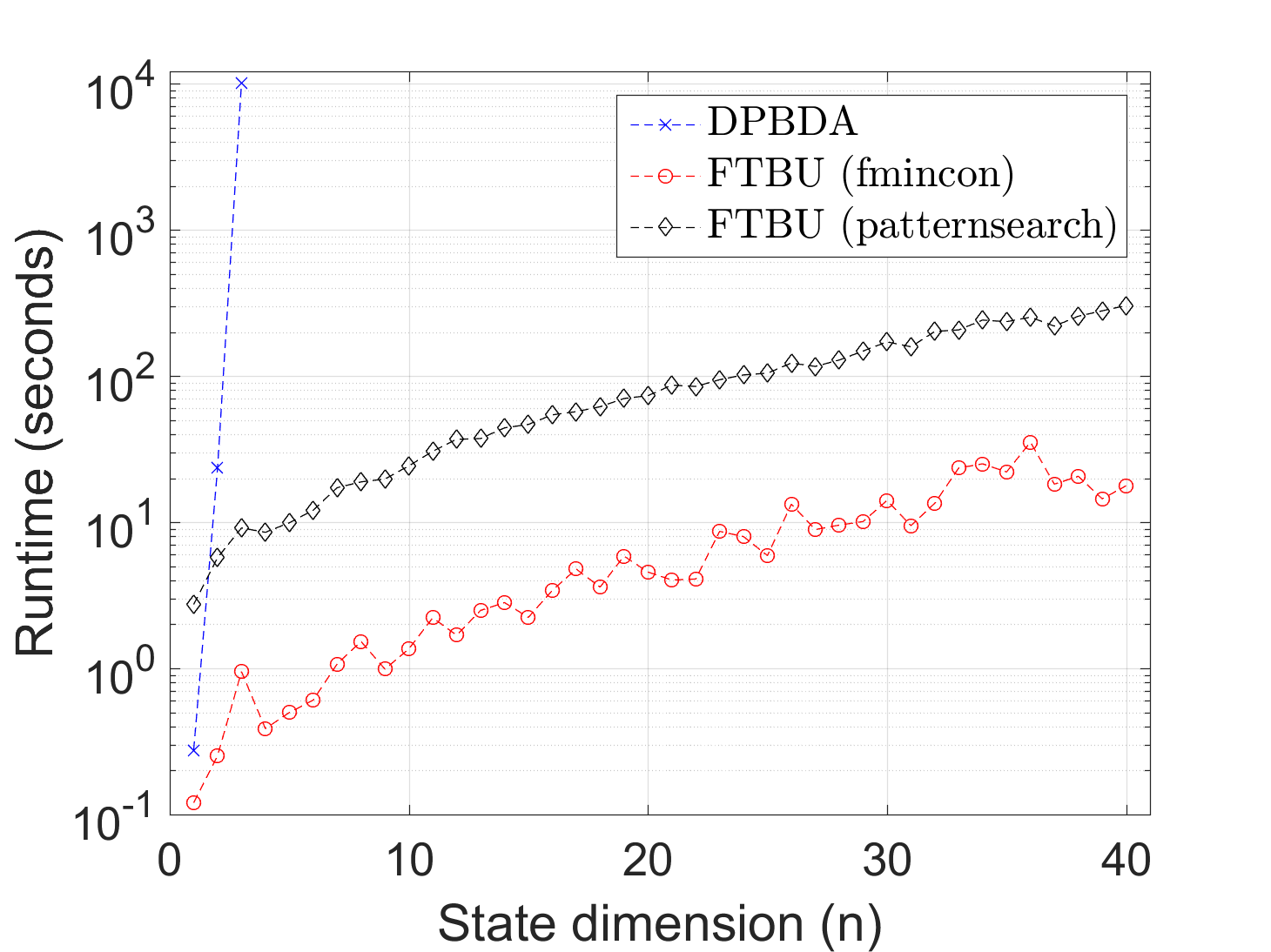
Figure 1: Scalability of DPBDA and FTBU with state dimension $n$ to compute $\hat{V}_{0}^{\ast}(\bar{x}_{0})$ and $\hat{W}_{0}^{\ast}(\bar{x}_{0})$ for some $\bar{x}_{0}\in\mathcal{X}$. Average computation time for the FTBU based on $20$ randomly chosen points in $\mathcal{T}$ at each $n$.

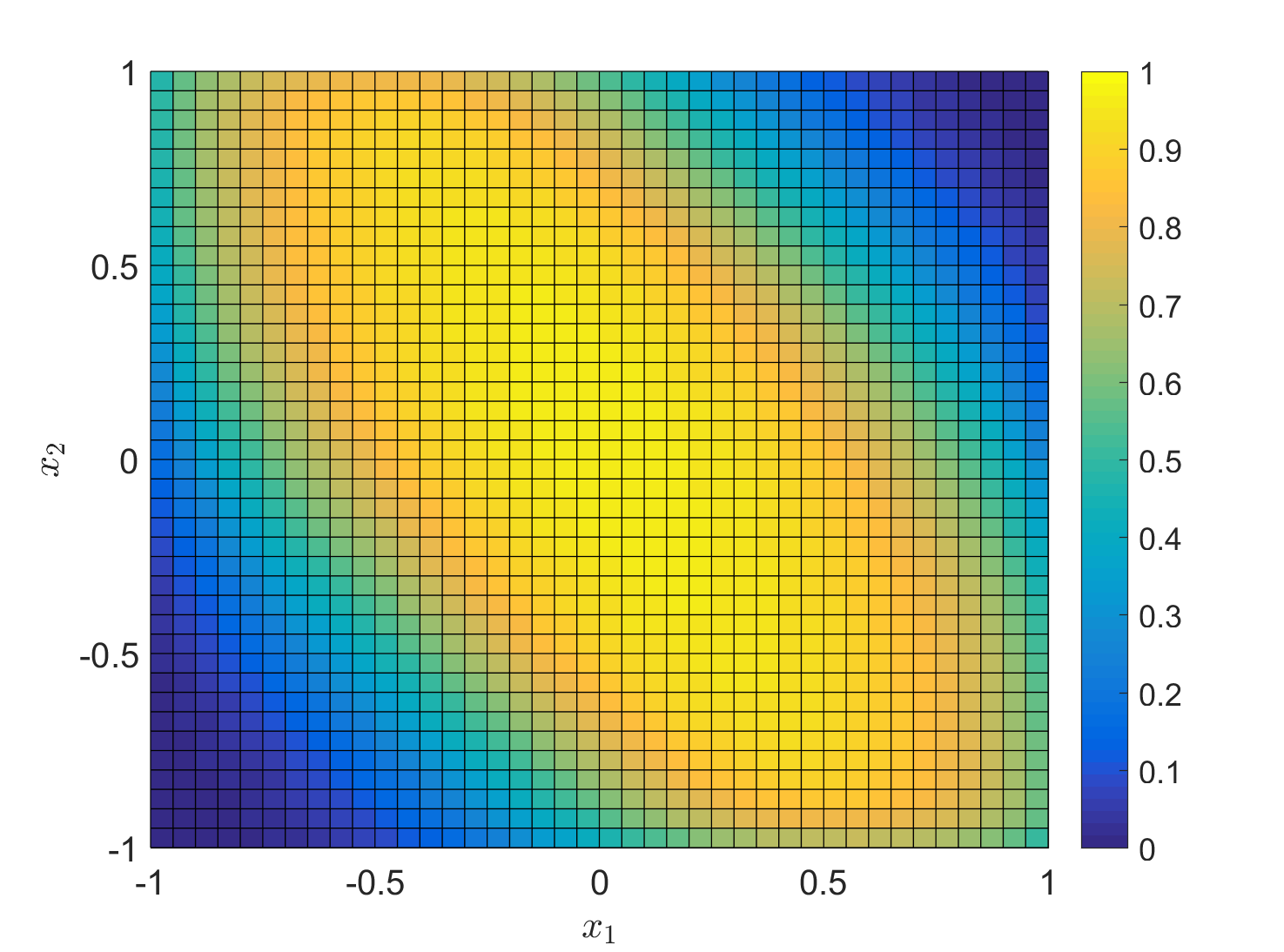
(a)

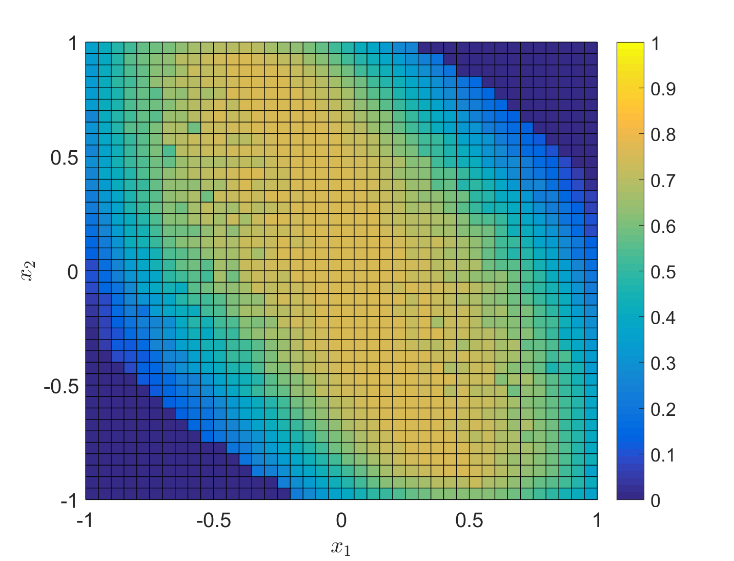
(b)

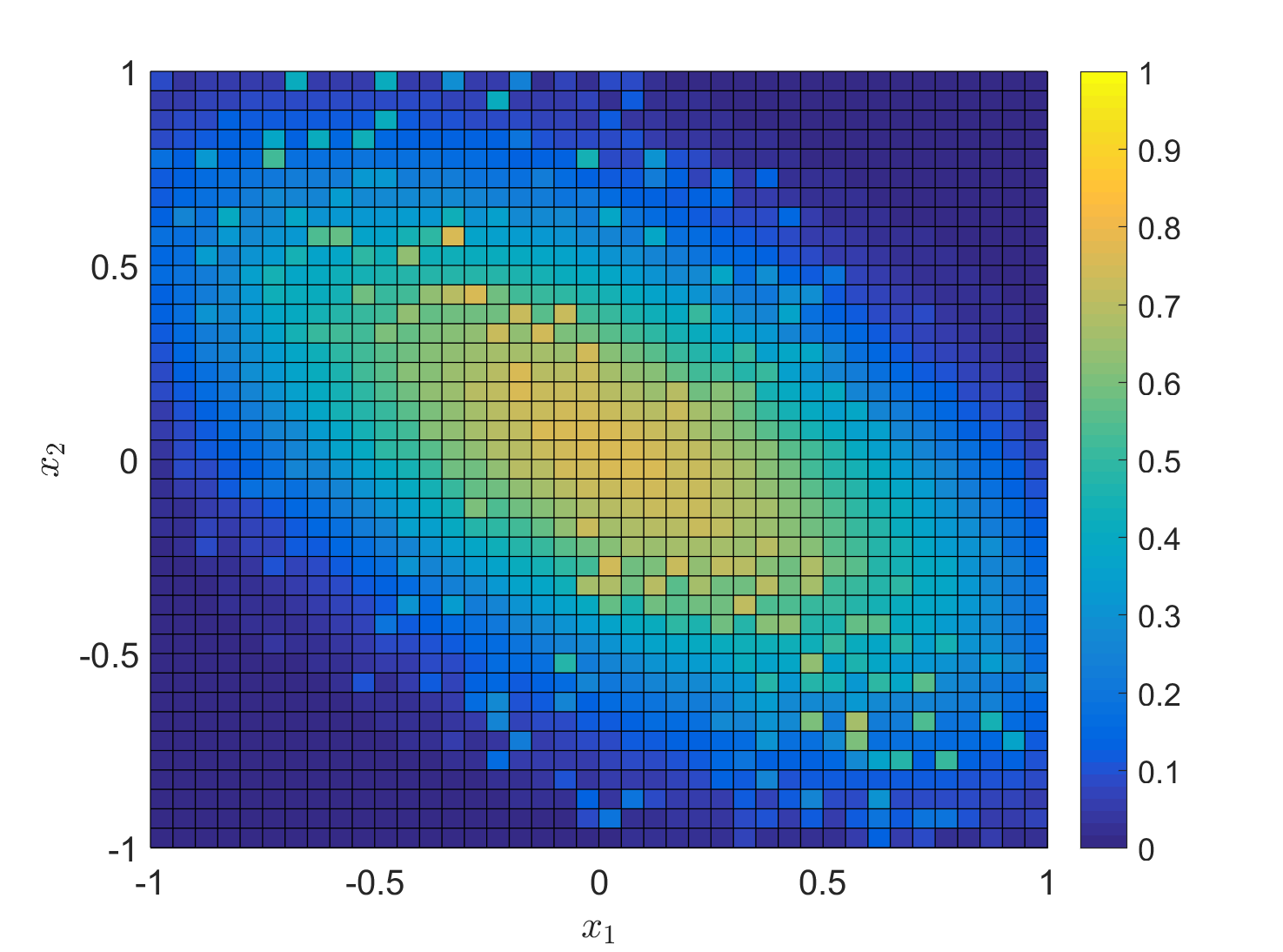
(c)

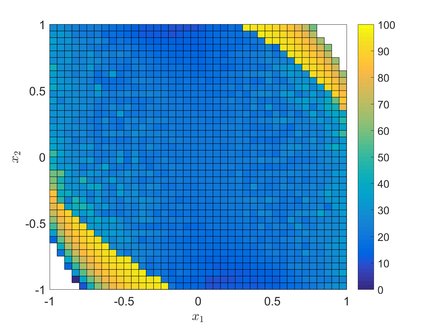
(d)

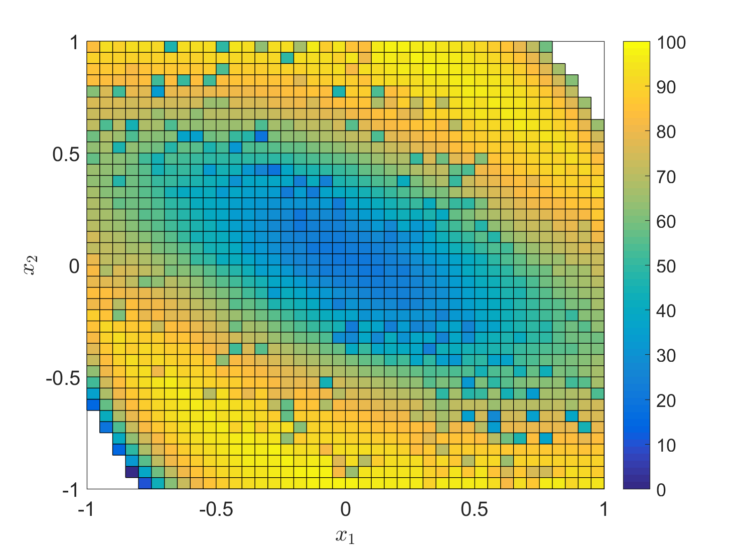
(e)

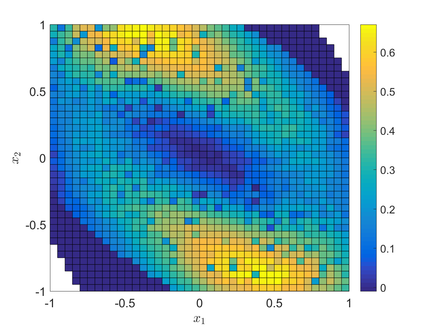
(f)

Figure 2: Conservativeness of the underapproximation for a double integrator ($n=2$). (a) Dynamic programming (DPBDA) approximation of $\hat{V}_{0}^{\ast}(\cdot)$; Fourier transform-based underapproximation (FTBU) $\hat{W}_{0}^{\ast}(\cdot)$ computed (b) using patternsearch and (c) using fmincon for each grid point; Relative error defined as $\frac{\hat{V}_{0}^{\ast}(\cdot)-\hat{W}_{0}^{\ast}(\cdot)}{\hat{V}_{0}^{\ast}(\cdot)}\times 100$ for $\hat{V}_{0}^{\ast}(\cdot)>\epsilon$ and $\hat{W}_{0}^{\ast}(\cdot)$ computed (d) using patternsearch and (e) using fmincon for each grid point; Note that higher errors occur closer to the boundary, as expected, due to the lack of feedback; (f) Improvement in $\hat{W}_{0}^{\ast}(\cdot)$ using patternsearch instead of fmincon; $\epsilon=0.01$

Table I summarizes the bounds on $\hat{V}_{0}^{\ast}(\cdot)$ for various $\bar{x}_{0}$ at $n=40$. For high $n$, (34) becomes severely under-actuated and the influence of the disturbance becomes very strong. This leads to the open-loop formulation yielding trivial lower bounds, $\hat{r}_{\bar{x}_{0}}^{\rho^{\ast}(\bar{x}_{0})}(\mathcal{S},\mathcal{T})=\epsilon$, for many $\bar{x}_{0}$ in the original $\mathcal{S},\mathcal{T}$. We therefore set $\mathcal{T}={[-8,8]}^{40}$ and $\mathcal{S}={[-10,10]}^{40}$. While Theorem 2 assures that $\hat{W}_{0}^{\ast}(\cdot)$ is a lower bound on $\hat{V}_{0}^{\ast}(\cdot)$, this bound is subject to $\epsilon$, hence the discrepancies between the numerical values for $\hat{W}_{0}^{\ast}(\cdot)$ and the lower bounds on $\hat{V}_{0}^{\ast}(\cdot)$. We use $\epsilon=0.001$.

Initial state of interest $\bar{x}_{0}^{\top}$	Member of	$\hat{W}_{0}^{\ast}(\bar{x}_{0})$		$\hat{V}_{0}^{\ast}(\bar{x}_{0})$	Runtime (s)
		fm	ps		fm	ps
$[0\ 0\ 0\ \ldots\ 0]$	$\mathcal{T}$	$1$	$1$	$[0.999,1]$	$12$	$302$
$[2.5\ 2.5\ 2.5\ \ldots]$	$\mathcal{T}$	$0.984$	$0.986$	$[0.985,1]$	$798$	$1196$
$[$-$8.5\ 8\$-$8.5\ 8\ \ldots]$	$\mathcal{S}\setminus\mathcal{T}$	$0.500$	$0.999$	$[0.998,1]$	$12$	$441$

TABLE I: Non-trivial bounds for $\hat{V}_{0}^{\ast}(\bar{x}_{0})$ ($\bar{x}_{0}\in\mathbb{R}^{40}$); fm and ps is FTBU with fmincon and patternsearch respectively.

V-B Conservativeness of FTBU

Figure 2(d) and (e) shows the relative error of FTBU with respect to DPBDA, with $\mathcal{T}={[-0.5,0.5]}^{2}$, $\mathcal{S}={[-1,1]}^{2}$, grid spacing of $0.05$, and $\epsilon=0.01$. FTBU implemented using patternsearch has $77.57\%$ grid points with the relative error less than $30\%$ as compared to $6.6\%$ grid points for fmincon-based FTBU. This is also reflected in Figure 2(a), (b), (c).

The sharp rise in Figure 2(d) is due to points where $\hat{W}_{0}^{\ast}(\bar{x}_{0})=\epsilon$ and $\hat{V}_{0}^{\ast}(\bar{x}_{0})>>\epsilon$, resulting in a large relative error. The conservativeness of FTBU highlights the role of feedback in increasing the terminal time probability for any $\bar{x}_{0}\in\mathcal{X}$. However, as seen in Table I, for sufficiently large $\mathcal{S},\mathcal{T}$, we obtain non-trivial lower bounds even for high-dimensional systems. Figure 2(f) and Table I show that FTBU with patternsearch clearly outperforms fmincon in the quality of the underapproximation, at the expense of computation time.

Lastly, note that the expected symmetry about the origin of the terminal time probability for the system (34) is not evident, unless a fine grid is used (Figure 2(a)). Table II shows that FTBU can serve as a “certificate” for the validity of the grid spacing in DPBDA by relying on the conservativeness established by Theorem 2. That is, the FTBU underapproximation provides a grid-independent lower bound on the value function $\hat{V}_{0}^{\ast}(\bar{x}_{0})$ computed using DBPDA. For example, for the double integrator, a grid spacing of $0.1$ will not give accurate results with DPBDA, since $\hat{V}_{0}^{\ast}(\bar{x}_{1})<\hat{W}_{0}^{\ast}(\bar{x}_{1})$ contradicts Theorem 2.

Grid spacing	$0.1$	$0.05$	$0.01$	$0.005$
$\hat{V}_{0}^{\ast}(\bar{x}_{1})$	$0.422$	$0.506$	$0.476$	$0.478$
$\hat{V}_{0}^{\ast}(\bar{x}_{2})$	$0.527$	$0.510$	$0.483$	$0.479$
Computation time (seconds)	$11.22$	$42.68$	$1206.59$	$5710.06$

TABLE II: Grid spacing in DPBDA ($n=2$, $\bar{x}_{1}=-\bar{x}_{2}={[0.1\ 0.9]}^{\top}$, $\mathcal{T}={[-0.5,0.5]}^{2}$, $\mathcal{S}={[-1,1]}^{2}$, $\hat{W}_{0}^{\ast}(\bar{x}_{1})=\hat{W}_{0}^{\ast}(\bar{x}_{2})=0.436$, $\epsilon=0.001$).

VI Conclusion

We show the conservativeness of the open-loop formulation of the finite time horizon terminal hitting time stochastic reach-avoid problem for stochastic linear systems, using conditional expectations and sufficient conditions for Borel-measurability of the value functions. The open-loop formulation converts the verification problem into a simpler optimization problem. The objective function is a multi-dimensional integral, and an analytical expression of the integrand can be obtained using Fourier transforms. For Gaussian disturbances, the objective function can be evaluated efficiently and the optimization problem is log-concave. Because the underapproximation technique does not rely on a grid, it mitigates the curse of dimensionality, and provides non-trivial lower bounds on the stochastic reach-avoid probability. The method is demonstrated on 40D dynamical system.

References

- [1] S. Summers and J. Lygeros, “Verification of discrete time stochastic hybrid systems: A stochastic reach-avoid decision problem,” Automatica, vol. 46, no. 12, pp. 1951–1961, 2010.
- [2] A. P. Vinod, B. HomChaudhuri, and M. Oishi, “Forward stochastic reachability analysis for uncontrolled linear systems using Fourier transforms,” in Hybrid Systems: Comp. & Control, pp. 35–44.
- [3] B. HomChaudhuri, A. P. Vinod, and M. Oishi, “Computation of forward stochastic reach sets: Application to stochastic, dynamic obstacle avoidance,” in American Control Conf., Seattle, WA, 2017.
- [4] N. Malone, K. Lesser, M. Oishi, and L. Tapia, “Stochastic reachability based motion planning for multiple moving obstacle avoidance,” in Proc. Hybrid Syst.: Comput. and Ctrl., 2014, pp. 51–60.
- [5] K. Lesser, M. Oishi, and R. Erwin, “Stochastic reachability for control of spacecraft relative motion,” in IEEE Conf. Dec. Ctrl., 2013, pp. 4705–4712.
- [6] N. Kariotoglou, D. M. Raimondo, S. J. Summers, and J. Lygeros, “Multi-agent autonomous surveillance: a framework based on stochastic reachability and hierarchical task allocation,” J. Dyn. Sys., Meas., Control, vol. 137, no. 3, pp. 031 008–031 008–14, 2014.
- [7] A. Abate, M. Prandini, J. Lygeros, and S. Sastry, “Probabilistic reachability and safety for controlled discrete time stochastic hybrid systems,” Automatica, vol. 44, no. 11, pp. 2724–2734, 2008.
- [8] A. Abate, S. Amin, M. Prandini, J. Lygeros, and S. Sastry, “Computational approaches to reachability analysis of stochastic hybrid systems,” in Proc. Hybrid Syst.: Comput. and Ctrl., 2007, pp. 4–17.
- [9] N. Kariotoglou, S. Summers, T. Summers, M. Kamgarpour, and J. Lygeros, “Approximate dynamic programming for stochastic reachability,” in Proc. European Ctrl. Conf., 2013, pp. 584–589.
- [10] N. Kariotoglou, K. Margellos, and J. Lygeros, “On the computational complexity and generalization properties of multi-stage and stage-wise coupled scenario programs,” Sys. & Ctr. Lett., vol. 94, pp. 63–69, 2016.
- [11] G. Manganini, M. Pirotta, M. Restelli, L. Piroddi, and M. Prandini, “Policy search for the optimal control of Markov Decision Processes: A novel particle-based iterative scheme,” IEEE Trans. Cybern., pp. 1–13, 2015.
- [12] J. Ding, M. Kamgarpour, S. Summers, A. Abate, J. Lygeros, and C. Tomlin, “A stochastic games framework for verification and control of discrete time stochastic hybrid systems,” Automatica, vol. 49, no. 9, pp. 2665–2674, 2013.
- [13] A. Genz, “Numerical computation of multivariate normal probabilities,” J. of Comp. and Graph. Stat., vol. 1, no. 2, pp. 141–149, 1992.
- [14] J. Gleason, A. Vinod, and M. Oishi, “Underapproximation of reach-avoid sets for discrete-time stochastic systems via Lagrangian methods,” in IEEE Conf. Dec. Ctrl., https://arxiv.org/abs/1704.03555.
- [15] J. A. Gubner, Probability and random processes for electrical and computer engineers. Cambridge Univ. Press, 2006.
- [16] Y. Chow and H. Teicher, Probability Theory: Independence, Interchangeability, Martingales, 3rd ed. Springer New York, 1997.
- [17] E. M. Stein and G. L. Weiss, Introduction to Fourier analysis on Euclidean spaces. Princeton Univ. Press, 1971, vol. 1.
- [18] H. Cramér, Mathematical methods of statistics. Princ. Univ. Pr., 1961.
- [19] D. Bertsekas and S. Shreve, Stochastic optimal control: The discrete time case. Academic Press, 1978.
- [20] J. Skaf and S. Boyd, “Design of affine controllers via convex optimization,” IEEE Trans. Auto. Ctr., vol. 55, no. 11, pp. 2476–87, 2010.
- [21] T. Tao, Analysis II, 2nd ed. Hindustan Book Agency, 2009.
- [22] A. S. Nowak, “Universally measurable strategies in zero-sum stochastic games,” The Annals of Probability, pp. 269–287, 1985.
- [23] C. J. Himmelberg, T. Parthasarathy, and F. S. VanVleck, “Optimal plans for dynamic programming problems,” Mathematics of Operations Research, vol. 1, no. 4, pp. 390–394, 1976.
- [24] A. P. Vinod and M. Oishi, “Scalable underapproximation for stochastic reach-avoid problem for high-dimensional LTI systems using Fourier transforms,” https://arxiv.org/abs/1703.02135.
- [25] W. Press, S. Teukolsky, W. Vetterling, and B. Flannery, Numerical recipes: The art of scientific computing. Cambridge Univ. Pr., 2007.
- [26] A. Genz and F. Bretz, Computation of multivariate normal and t probabilities. Springer Science & Business Media, 2009, vol. 195.
- [27] S. Dharmadhikari and K. Joag-Dev, Unimodality, convexity, and applications. Elsevier, 1988.
- [28] S. Boyd and L. Vandenberghe, Convex optimization. Cambridge Univ. Press, 2004.
- [29] A. Genz, “QSCMVNV.” [Online]. Available: http://www.math.wsu.edu/faculty/genz/software/matlab/qscmvnv.m
- [30] T. G. Kolda, R. M. Lewis, and V. Torczon, “Optimization by direct search: New perspectives on some classical and modern methods,” SIAM review, vol. 45, no. 3, pp. 385–482, 2003.