Global behaviour of radially symmetric solutions stable at infinity for gradient systems

Abstract

This paper is concerned with radially symmetric solutions of parabolic gradient systems of the form

$$u_{t}=-\nabla V(u)+\Delta_{x}u$$

where the space variable $x$ and the state variable $u$ are multidimensional, and the potential $V$ is coercive at infinity. For such systems, under generic assumptions on the potential, the asymptotic behaviour of solutions stable at infinity, that is approaching a stable homogeneous equilibrium as $\left\lvert x\right\rvert$ goes to $+\infty$, is investigated. It is proved that every such solution approaches a pattern made of a stacked family of radially symmetric bistable fronts travelling to infinity, and around the origin a (possibly non-homogeneous) radially symmetric stationary solution. This behaviour is similar to that of bistable solutions for gradient systems in one unbounded spatial dimension, which is described in companion papers.

1 Introduction

This paper deals with the global dynamics of radially symmetric solutions of nonlinear parabolic systems of the form

(1.1) $$\tilde{u}_{t}=-\nabla V(\tilde{u})+\Delta_{x}\tilde{u}$$

where the time variable $t$ is real, the space variable $x$ lies in the spatial domain $\mathbb{R}^{d}$ with $d$ a positive integer, the function $(x,t)\mapsto\tilde{u}(x,t)$ takes its values in $\mathbb{R}^{{d_{\textup{\text{st}}}}}$ with ${d_{\textup{\text{st}}}}$ a positive integer, and the nonlinearity is the gradient of a scalar potential function $V:\mathbb{R}^{{d_{\textup{\text{st}}}}}\to\mathbb{R}$, which is assumed to be regular (of class $\mathcal{C}^{2}$) and coercive at infinity (see hypothesis $\text{H}_{\text{coerc}}$ in 2.1).

Notation.

As the previous sentence shows, the state dimension is thus denoted by ${d_{\textup{\text{st}}}}$ whereas the space dimension is simply denoted by $d$. The reason for this choice (and for the absence of subscript in the notation for the space dimension) is that, by contrast with the state dimension, the space dimension is ubiquitous in the computations throughout the paper.

Radially symmetric solutions of system 1.1 are functions of the form

$$\tilde{u}(x,t)=u(r,t)\,,\quad\text{where }r=\left\lvert x\right\rvert\text{ (the euclidean norm of }x\text{ in }\mathbb{R}^{d}\text{),}$$

and $(r,t)\mapsto u(r,t)$ is defined on $[0,+\infty)\times[0,+\infty)$ with values in $\mathbb{R}^{{d_{\textup{\text{st}}}}}$. For such functions, system 1.1 takes the following form:

(1.2) $$u_{t}=-\nabla V(u)+\frac{d-1}{r}u_{r}+u_{rr}\quad\text{with the boundary condition}\quad\partial_{r}u(0,t)=0\,,$$

and it this last system 1.2 that will be considered in this paper.

A fundamental feature of each of systems 1.1 and 1.2 is that they can be recast, at least formally, as gradient flows of energy functionals. If $(w,w^{\prime})$ is a pair of vectors of $\mathbb{R}^{{d_{\textup{\text{st}}}}}$, let $w\cdot w^{\prime}$ and $\left\lvert w\right\rvert=\sqrt{w\cdot w}$ denote the usual Euclidean scalar product and the usual Euclidean norm, respectively, and let us simply write $w^{2}$ for $\left\lvert w\right\rvert^{2}$.

For every function $x\mapsto\tilde{v}(x)$ defined on $\mathbb{R}^{d}$ with values in $\mathbb{R}^{{d_{\textup{\text{st}}}}}$, its energy (or Lagrangian or action) with respect to system 1.1 is defined (at least formally) by

$$\tilde{\mathcal{E}}[\tilde{v}]=\int_{\mathbb{R}^{d}}\biggl{(}\frac{1}{2}\left\lvert\nabla_{x}\tilde{v}(x)\right\rvert^{2}+V\bigl{(}\tilde{v}(x)\bigr{)}\biggr{)}\,dx$$

where

$$\left\lvert\nabla_{x}\tilde{v}(x)\right\rvert^{2}=\sum_{i=1}^{d}\sum_{j=1}^{{d_{\textup{\text{st}}}}}\bigl{(}\partial_{x_{i}}\tilde{v}_{j}(x)\bigr{)}^{2}\,.$$

Similarly, for every function $r\mapsto v(r)$ defined on $[0,+\infty)$ with values in $\mathbb{R}^{{d_{\textup{\text{st}}}}}$, its energy (or Lagrangian or action) with respect to system 1.2 is defined (at least formally) by

(1.3) $$\mathcal{E}[v]=\int_{0}^{+\infty}r^{d-1}\Bigl{(}\frac{1}{2}v_{r}(r)^{2}+V\bigl{(}v(r)\bigr{)}\Bigr{)}\,dr\,.$$

Note that if $\tilde{v}:\mathbb{R}^{d}\to\mathbb{R}$ denotes a (radially symmetric) function defined as $\tilde{v}(x)=v(\left\lvert x\right\rvert)$, and if $S_{d-1}$ denotes the surface area of the $d-1$-unit-sphere in $\mathbb{R}^{d}$, then

(1.4) $$\tilde{\mathcal{E}}[\tilde{v}]=S_{d-1}\,\mathcal{E}[v]\,.$$

Formally, the differential of the functional $\mathcal{E}$ defined by 1.3 reads (skipping border terms in the integration by parts):

$$d\mathcal{E}[v]\cdot\delta v =\int_{0}^{+\infty}r^{d-1}\bigl{(}v_{r}\cdot(\delta v)_{r}+\nabla V(v)\cdot\delta v\bigr{)}\,dr$$

$$=\int_{0}^{+\infty}r^{d-1}\Bigl{(}-v_{rr}-\frac{d-1}{r}v_{r}+\nabla V(v)\Bigr{)}\cdot\delta v\,dr\,.$$

In other words, the (formal) gradient of this functional with respect to the $L^{2}$-scalar product with weight $r^{d-1}$ on functions $[0,+\infty)\to\mathbb{R}^{{d_{\textup{\text{st}}}}}$ reads:

$$\nabla_{\text{rad}}\mathcal{E}[v]=-v_{rr}-\frac{d-1}{r}v_{r}+\nabla V(v)\,,$$

thus system 1.2 can formally be rewritten under the form:

$$u_{t}=-\nabla_{\text{rad}}\mathcal{E}[u(\cdot,t)]\,,$$

and if $(r,t)\mapsto u(r,t)$ is a solution of this system, then (formally)

$$\frac{d}{dt}\mathcal{E}[u(\cdot,t)]=-\int_{0}^{+\infty}r^{d-1}u_{t}(r,t)^{2}\,dr\leq 0\,.$$

An additional and related feature of system 1.1 is that a formal gradient structure exists not only in the laboratory frame, but also in every frame travelling at a constant velocity, [56]. What about radially symmetric solutions of system 1.2 with respect to the radial coordinate $r$? Let us see this now.

For every nonnegative quantity $c$, if $(r,t)\mapsto u(r,t)$ and $(\rho,t)\mapsto v(\rho,t)$ are two functions related by

$$u(r,t)=v(\rho,t)\quad\text{for}\quad r=ct+\rho\,,$$

then $u$ is a solution of 1.2 if and only if $v$ is a solution of

(1.5) $$v_{t}-c\cdot v_{\rho}=-\nabla V(v)+\frac{d-1}{ct+\rho}v_{\rho}+v_{\rho\rho}\,.$$

Now, for every function $w:\rho\mapsto w(\rho)$ defined on $[-ct,+\infty)$ with values in $\mathbb{R}^{{d_{\textup{\text{st}}}}}$, its energy functional with respect to system 1.5 may be defined, at least formally, as

(1.6) $$\mathcal{E}_{c,t}[w]=\int_{-ct}^{+\infty}(ct+\rho)^{d-1}e^{c\rho}\Bigl{(}\frac{1}{2}w_{\rho}(\rho)^{2}+V\bigl{(}w(\rho)\bigr{)}\Bigr{)}\,d\rho\,.$$

Formally, the differential of this functional reads (skipping border terms in the integration by parts)

$$d\mathcal{E}_{c,t}[w]\cdot\delta w =\int_{-ct}^{+\infty}(ct+\rho)^{d-1}e^{c\rho}\bigl{(}w_{\rho}\cdot\delta w_{\rho}+\nabla V(w)\cdot\delta w\bigr{)}\,d\rho$$

$$=\int_{-ct}^{+\infty}(ct+\rho)^{d-1}e^{c\rho}\Bigl{(}-w_{\rho\rho}-cw_{\rho}-\frac{d-1}{ct+\rho}w_{\rho}+\nabla V(w)\Bigr{)}\cdot\delta w\,d\rho\,.$$

In other words, the (formal) gradient of this functional with respect to the $L^{2}$-scalar product with weight $(ct+\rho)^{d-1}e^{c\rho}$ on functions $[-ct,+\infty)\to\mathbb{R}^{{d_{\textup{\text{st}}}}}$ reads:

$$\nabla_{\text{rad},c}\mathcal{E}_{c,t}[w]=-w_{\rho\rho}-cw_{\rho}-\frac{d-1}{ct+\rho}w_{\rho}+\nabla V(w)\,,$$

and system 1.5 can formally be rewritten under the form:

(1.7) $$v_{t}=-\nabla_{\text{rad},c}\mathcal{E}_{c,t}[v(\cdot,t)]\,.$$

Now, if $(\rho,t)\mapsto v(\rho,t)$ is a solution of system 1.5, then (formally):

(1.8) $$\frac{d}{dt}\mathcal{E}_{c,t}[v(\cdot,t)]=\int_{-ct}^{+\infty}(ct+\rho)^{d-1}e^{c\rho}\Biggl{[}-v_{t}(\rho,t)^{2}+\frac{c(d-1)}{ct+\rho}\Bigl{(}\frac{1}{2}v_{\rho}^{2}+V(v)\Bigr{)}\Biggr{]}\,d\rho\,.$$

What can be seen from these calculations is that, although system 1.5 is still formally gradient, the time derivative of the energy 1.6 involves, in addition to the standard dissipation term $-v_{t}^{2}$, an additional term, that can be related to the time dependence of the $L^{2}$-scalar product defining the gradient $\nabla_{\text{rad},c}$, or viewed as induced by the curvature $1/r=1/ct+\rho$. Only in the limit of large radii (or large positive times, or small curvature) is the expression of the time derivative of energy always nonnegative. In short, the picture is not hopeless, but not as nice as it would be in space dimension $1$.

This gradient structure (“asymptotic” gradient structure in the case of system 1.5) has been known for a long time [17], but it is only more recently that it received a more detailed attention from several authors (among which S. Heinze, C. B. Muratov, Th. Gallay, R. Joly, and the author [25, 36, 21, 52, 20]), and that is was shown that this structure is sufficient (in itself, that is without the use of the maximum principle) to prove results of global convergence towards travelling fronts. These ideas have been applied since in different contexts, to prove either global convergence or just existence results, see for instance [9, 10, 37, 38, 39, 2, 1, 30, 8, 6, 7, 42, 43, 12, 11, 44].

Even more recently, the same ideas enabled the author ([57, 54]) to push one step further (that is, extend to systems) the program initiated by P. C. Fife and J. McLeod in the late seventies with the aim of describing the global asymptotic behaviour (when space is one-dimensional) of every bistable solution, that is every solution close to stable homogeneous equilibria at both ends of space ([17, 18, 19]). Under generic assumptions on the potential $V$, these solutions approach a stacked (possibly empty) family of bistable travelling fronts at both ends of space, and approach in between a pattern of stationary solutions going slowly away from one another. These stacked families will be called terraces (see sub-subsection 2.3.4 for comments and references on this terminology and a precise definition in the framework of this paper).

The aim of this paper is to extend to the case of radially symmetric solutions in higher space dimensions the results (description of the global asymptotic behaviour) obtained in [57, 54] for bistable solutions when spatial domain is one-dimensional. Thus, the solutions that will be considered are solutions of system 1.2 that approach a stable homogeneous equilibrium as the radius $r$ goes to $+\infty$ (or equivalently radially symmetric solutions of system 1.1 that are stable at infinity, in space). The goal is to prove that, under generic assumptions on the potential, every such solution approaches a pattern made of a stacked family of (radially symmetric) bistable front going to infinity (a “propagating terrace”), and around the origin a radially symmetric stationary solution (which may or not be spatially homogeneous).

In the scalar case ${d_{\textup{\text{st}}}}$ equals $1$, the behaviour of solutions stable at infinity of reaction-diffusion equations in higher space dimension is the subject of a large amount of literature. For extinction/invasion (threshold) results in relation with the initial condition and the reaction term see for instance [3, 13, 40, 41, 61], for local convergence and quasi-convergence results see for instance [13, 15, 31, 33, 48, 24], and for further estimates on the location and shape at large positive times of the level sets see for instance [29, 28, 60, 59, 58, 24]. Recently, a result of global convergence towards a radial terrace of travelling fronts was proved by Y. Du and H. Matano [14] (without any radial symmetry assumption on the solutions), and a rather complementary result of convergence/quasi-convergence (in $L^{\infty}_{\text{loc}}(\mathbb{R}^{{d_{\textup{\text{st}}}}},\mathbb{R})$) was proved by P. Poláčik [51] under very weak non-degeneracy assumptions on the nonlinearity; see also [34, 35] for results similar to those of [14] when space is anisotropic. The present paper extends some of those results (in particular some of the results of [14, 51]) to the more general setting of systems, but for radially symmetric solutions only.

The path of the proof is very similar to the one used in the spatial dimension one case [57, 54]. It is based on a careful study of the relaxation properties of energy or $L^{2}$ functionals (localized in space by adequate weight functions), both in the laboratory frame and in frames travelling at various speeds. The differences are mainly of technical nature due to specific features of the (reduced) system 1.2:

• the “curvature” term $(d-1)u_{r}/r$;

• the fact that space is reduced to the half-line $[0,+\infty)$ (thus is in this sense less “spatially homogeneous” than the full real line);

• the “no invasion implies relaxation” part of the argument, which does not call upon the radial symmetry and is therefore processed in the companion paper [56];

• the convergence behind the terrace of travelling front, which differs from the space dimension one case both regarding the arguments and the result (roughly speaking, again due to the curvature term).

2 Assumptions, notation, and statement of the results

This section presents strong similarities with [54, section 2] and [57, section 2], where more details and comments can be found.

For the remaining of the paper it will be assumed than the space dimension $d$ is not smaller than $2$. Indeed the case $d=1$ was already treated in [57, 54], and several definitions, estimates, and statements will turn out to be irrelevant without this assumption (see for instance the definition of the weight function $T_{\rho}\psi_{0}$ in 4.4.1).

2.1 Semi-flow and coercivity hypothesis

Let us consider the following two Banach spaces of continuous and uniformly bounded functions equipped with the uniform norm:

$$X =\bigl{(}\mathcal{C}^{0}_{\textup{\text{b}}}\bigl{(}\mathbb{R}^{d},\mathbb{R}^{{d_{\textup{\text{st}}}}}\bigr{)},\left\lVert\dots\right\rVert_{L^{\infty}(\mathbb{R}^{d},\mathbb{R}^{{d_{\textup{\text{st}}}}})}\bigr{)}\,,$$

$$\text{and}\quad Y =\Bigl{(}\mathcal{C}^{0}_{\textup{\text{b}}}\bigl{(}[0,+\infty),\mathbb{R}^{{d_{\textup{\text{st}}}}}\bigr{)},\left\lVert\dots\right\rVert_{L^{\infty}\bigl{(}[0,+\infty),\mathbb{R}^{{d_{\textup{\text{st}}}}}\bigr{)}}\Bigr{)}\,.$$

System 1.1 defines a local semi-flow in $X$ (see for instance D. B. Henry’s book [26]).

As in [57, 54], let us assume that the potential function $V:\mathbb{R}^{{d_{\textup{\text{st}}}}}\to\mathbb{R}$ is of class $\mathcal{C}^{2}$ and that this potential function is strictly coercive at infinity in the following sense:

($$\text{H}_{\text{coerc}} \lim_{R\to+\infty}\quad\inf_{\left\lvert u\right\rvert\geq R}\ \frac{u\cdot\nabla V(u)}{\left\lvert u\right\rvert^{2}}>0$$)

(or in other words there exists a positive quantity $\varepsilon$ such that the quantity $u\cdot\nabla V(u)$ is greater than or equal to $\varepsilon\left\lvert u\right\rvert^{2}$ as soon as $\left\lvert u\right\rvert$ is large enough).

According to this hypothesis $\text{H}_{\text{coerc}}$, the semi-flow of system 1.1 on $X$ is actually global (see 3.1). As a consequence, considering the restriction of this semi-flow to radially symmetric functions, it follows that system 1.2 defines a global semi-flow on $Y$. Let us denote by $(S_{t})_{t\geq 0}$ this last semi-flow on $Y$.

In the following, a solution of system 1.2 will refer to a function

$$[0,+\infty)\times[0,+\infty)\to\mathbb{R}^{{d_{\textup{\text{st}}}}}\,,\quad(r,t)\mapsto u(r,t)\,,$$

such that the function $u_{0}:r\mapsto u(r,t=0)$ (initial condition) is in $Y$ and $u(\cdot,t)$ equals $(S_{t}u_{0})(\cdot)$ for every nonnegative time $t$.

2.2 Minimum points and solutions stable at infinity

2.2.1 Minimum points

Everywhere in this paper, the term “minimum point” denotes a point where a function — namely the potential $V$ — reaches a local or global minimum. Let $\mathcal{M}$ denote the set of nondegenerate minimum points:

$$\mathcal{M}=\{u\in\mathbb{R}^{{d_{\textup{\text{st}}}}}:\nabla V(u)=0\quad\text{and}\quad D^{2}V(u)\text{ is positive definite}\}\,.$$

2.2.2 Solutions stable at infinity

Definition 2.1 (solution stable at infinity).

A solution $(r,t)\mapsto u(r,t)$ of system 1.2 is said to be stable at infinity if there exists a point $m$ in $\mathcal{M}$ such that

$$\limsup_{r\to+\infty}\left\lvert(u(r,t)-m\right\rvert\to 0\quad\text{as}\quad t\to+\infty\,.$$

More precisely, such a solution is said to be stable close to $m$ at infinity. A function (initial condition) $u_{0}$ in $Y$ is said to be stable (close to $m$) at infinity if the solution of system 1.2 corresponding to this initial condition is stable (close to $m$) at infinity.

Notation.

Let

$$Y_{\textup{\text{stab-infty}}}(m)$$

denote the subset of $Y$ made of initial conditions that are stable close to $m$ at infinity.

2.3 Stationary solutions, travelling fronts, terraces, and asymptotic pattern

2.3.1 Radially symmetric stationary solutions

A function

$$\phi:[0,+\infty)\to\mathbb{R}^{{d_{\textup{\text{st}}}}},\quad r\mapsto\phi(r)$$

is a stationary solution of system 1.2 if $\phi$ is a solution of the differential system

(2.1) $$\phi^{\prime\prime}+\frac{d-1}{r}\phi^{\prime}=\nabla V(\phi)\,,\quad\text{with the boundary condition}\quad\phi^{\prime}(0)=0\,.$$

Notation.

If $m$ is in $\mathcal{M}$, let $\Phi_{0,\textup{\text{centre}}}(m)$ denote the set of solutions of system 2.1 approaching $m$ at infinity. With symbols,

(2.2) $$\Phi_{0,\textup{\text{centre}}}(m)=\bigl{\{} \phi:[0,+\infty)\to\mathbb{R}^{{d_{\textup{\text{st}}}}}:\phi\text{ is a solution of system \lx@cref{creftype~refnum}{syst_rad_sym_stationary}}$$

$$\text{and}\quad\phi(r)\xrightarrow[r\to+\infty]{}m\bigr{\}}\,.$$

In this notation,

• the index “$0$” refers to the “zero speed” of these solutions, by contrast with the nonzero speed of the travelling fronts considered below,

• the symbols $\Phi$ and $\phi$ have been chosen for homogeneity with the notation introduced below for travelling fronts,

• and the index “centre” refers to the fact that these solutions are stationary for system 1.2 (with the curvature term) and not for system 2.4 introduced below.

This set $\Phi_{0,\textup{\text{centre}}}(m)$ comprises the constant solution $\phi\equiv m$, by contrast with the sets introduced in the next two sub-subsections 2.3.3 and 2.4.2.

A function $\phi$ belonging to $\Phi_{0,\textup{\text{centre}}}(m)$ for some $m$ in $\mathcal{M}$ is said to be stable at infinity.

Definition 2.2 (energy of a stationary solution stable at infinity).

If $m$ is a point in $\mathcal{M}$ and $\phi$ is a function in $\Phi_{0,\textup{\text{centre}}}(m)$, let us call energy of $\phi$, and let us denote by $\mathcal{E}[\phi]$, the quantity

$$\mathcal{E}[\phi]=\int_{0}^{+\infty}r^{d-1}\Bigl{(}\frac{1}{2}\phi^{\prime}(r)^{2}+V\bigl{(}\phi(r)\bigr{)}-V(m)\Bigr{)}\,dr\,.$$

Since $\phi(r)$ goes to $m$ at an exponential rate as $r$ goes to $+\infty$, this integral converges.

It follows from Pokhozhaev’s identity ([46, 4]) that

(2.3) $$\mathcal{E}[\phi]=\frac{1}{d}\int_{0}^{+\infty}r^{d-1}\phi^{\prime}(r)^{2}\,dr\,,$$

and this shows that $\mathcal{E}[\Phi]$ is nonnegative (and even positive if $\phi$ is not identically equal to $m$). It turns out that the results of the companion paper [56] provide another justification of the nonnegativity of this energy (see conclusion 1 of Proposition 5.1).

Remark.

Let us denote by $S_{d-1}$ the surface area of the $d-1$-unit sphere in $\mathbb{R}^{d}$, and let us introduce the function $\tilde{\phi}:\mathbb{R}^{d}\to\mathbb{R}$ defined as $\tilde{\phi}(x)=\phi(\left\lvert x\right\rvert)$; then,

$$S_{d-1}\,\mathcal{E}[\phi]=\int_{\mathbb{R}^{d}}\Bigl{(}\frac{1}{2}\left\lvert\nabla\tilde{\phi}(x)\right\rvert^{2}+V\bigl{(}\tilde{\phi}(x)\bigr{)}-V(m)\Bigr{)}\,dx$$

(compare with equality 1.4 in introduction).

2.3.2 Large radius asymptotic form of the system governing radially symmetric solutions

When the radius $r$ goes to $+\infty$, system 1.2 governing radially symmetric solutions takes the following asymptotic form:

(2.4) $$u_{t}=-\nabla V(u)+u_{rr}\,,$$

on functions $(r,t)\mapsto u(r,t)$ defined on $\mathbb{R}\times[0,+\infty)$ (here the radius $r$ is defined on the whole real line), with values in $\mathbb{R}^{{d_{\textup{\text{st}}}}}$.

2.3.3 Radially symmetric travelling fronts for the large radius limit

Let $c$ be a positive quantity. A function

$$\phi:\mathbb{R}\to\mathbb{R}^{{d_{\textup{\text{st}}}}},\quad\rho\mapsto\phi(\rho)$$

is the profile of a wave travelling at the speed $c$ for system 2.4 if the function $(r,t)\mapsto\phi(r-ct)$ is a solution of this system, that is if $\phi$ is a solution of the differential system

(2.5) $$\phi^{\prime\prime}=-c\phi^{\prime}+\nabla V(\phi)\,.$$

Notation.

If $m_{-}$ and $m_{+}$ are two points of $\mathcal{M}$ and $c$ is a positive quantity, let $\Phi_{c}(m_{-},m_{+})$ denote the set of nonconstant global solutions of system 2.5 connecting $m_{-}$ to $m_{+}$. With symbols,

$$\Phi_{c}(m_{-},m_{+})=\bigl{\{} \phi:\mathbb{R}\to\mathbb{R}^{{d_{\textup{\text{st}}}}}:\phi\text{ is a \emph{nonconstant} global solution of system \lx@cref{creftype~refnum}{syst_trav_front}}$$

$$\text{and}\quad\phi(\rho)\xrightarrow[\rho\to-\infty]{}m_{-}\quad\text{and}\quad\phi(\rho)\xrightarrow[\rho\to+\infty]{}m_{+}\bigr{\}}\,.$$

If $\phi$ is an element of some set $\Phi_{c}(m_{-},m_{+})$ for some positive quantity $c$, then it follows from system 2.5 that

(2.6) $$V(m_{+})-V(m_{-})=c\int_{\mathbb{R}}\phi^{\prime}(\xi)^{2}\,d\xi\,,$$

so that $V(m_{-})$ is less than $V(m_{+})$ and $m_{-}$ and $m_{+}$ differ; in this case the function $\phi$ is thus the profile of a travelling front. Since its asymptotic values $m_{-}$ and $m_{+}$ belong to $\mathcal{M}$, this front is qualified as bistable.

2.3.4 Propagating terraces of bistable travelling fronts

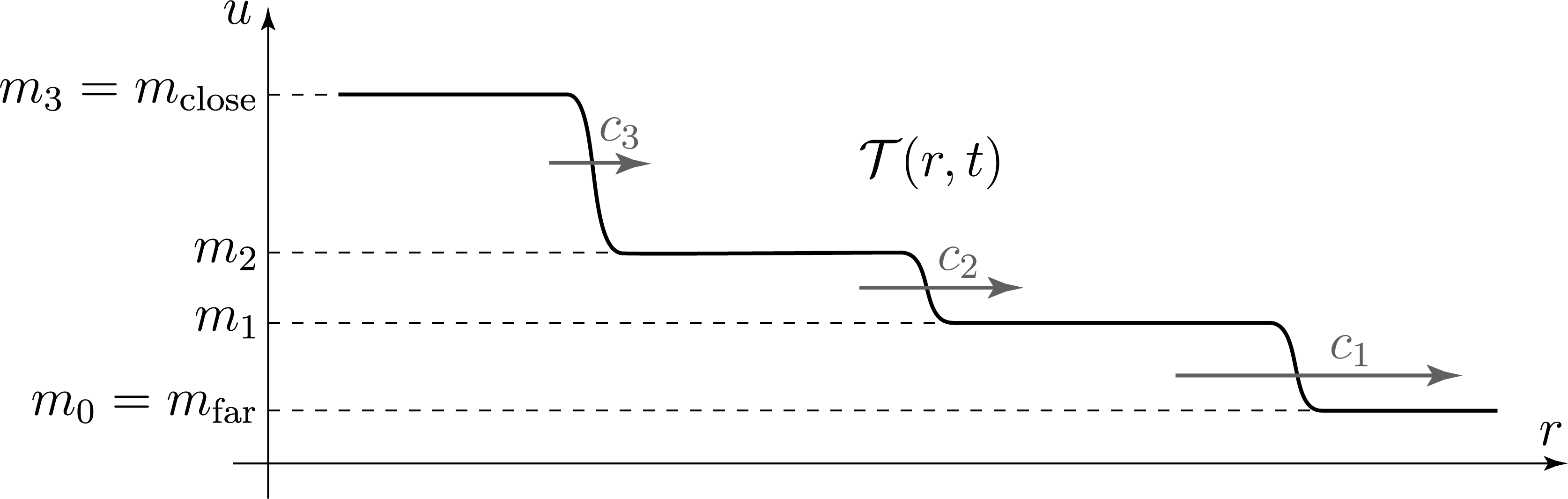
Figure 2.1: Propagating terrace of (bistable) fronts (travelling to the right).

Definition 2.3 (propagating terrace of bistable travelling fronts, figure 2.1).

Let $m_{\textup{\text{close}}}$ and $m_{\textup{\text{far}}}$ be two points of $\mathcal{M}$ (satisfying $V(m_{\textup{\text{close}}})\leq V(m_{\textup{\text{far}}})$). A function

$$\mathcal{T}:\mathbb{R}\times[0,+\infty)\to\mathbb{R}^{{d_{\textup{\text{st}}}}},\quad(r,t)\mapsto\mathcal{T}(r,t)$$

is called a propagating terrace of bistable fronts travelling to the right, connecting $m_{\textup{\text{close}}}$ to $m_{\textup{\text{far}}}$, if there exists a nonnegative integer $q$ such that:

1. if $q$ equals $0$, then $m_{\textup{\text{close}}}=m_{\textup{\text{far}}}$ and, for every real quantity $r$ and every nonnegative time $t$,

   $$\mathcal{T}(r,t)=m_{\textup{\text{close}}}=m_{\textup{\text{far}}}\,;$$

2. if $q$ equals $1$, then there exist

   • a positive quantity $c_{1}$

   • and a function $\phi_{1}$ in $\Phi_{c}(m_{\textup{\text{close}}},m_{\textup{\text{far}}})$ (that is, the profile of a bistable front travelling at the speed $c_{1}$ and connecting $m_{\textup{\text{close}}}$ to $m_{\textup{\text{far}}}$)

   • and a $\mathcal{C}^{1}$-function $[0,+\infty)\to[0,+\infty)$, $t\mapsto r_{1}(t)$, satisfying $r_{1}^{\prime}(t)\to c_{1}$ as time goes to $+\infty$

   such that, for every real quantity $r$ and every nonnegative time $t$,

   $$\mathcal{T}(r,t)=\phi_{1}\bigl{(}r-r_{1}(t)\bigr{)}\,;$$

3. if $q$ is not smaller than $2$, then there exists $q-1$ points $m_{1},\dots,m_{q-1}$ of $\mathcal{M}$, satisfying (if $m_{\textup{\text{far}}}$ is denoted by $m_{0}$ and $m_{\textup{\text{close}}}$ by $m_{q}$)

   $$V(m_{0})>V(m_{1})>\dots>V(m_{q})\,,$$

   and there exist $q$ positive quantities $c_{1}$, …, $c_{q}$ satisfying:

   $$c_{1}\geq\dots\geq c_{q}\,,$$

   and for every integer $i$ in $\{1,\dots,q\}$, there exist:

   • a function $\phi_{i}$ in $\Phi_{c_{i}}(m_{i},m_{i-1})$ (that is, the profile of a bistable front travelling at the speed $c_{i}$ and connecting $m_{i}$ to $m_{i-1}$)

   • and a $\mathcal{C}^{1}$-function $[0,+\infty)\to[0,+\infty)$, $t\mapsto r_{i}(t)$, satisfying $r_{i}^{\prime}(t)\to c_{i}$ as time goes to $+\infty$

   such that, for every integer $i$ in $\{1,\dots,q-1\}$,

   $$r_{i+1}(t)-r_{i}(t)\to+\infty\quad\text{as}\quad t\to+\infty\,,$$

   and such that, for every real quantity $r$ and every nonnegative time $t$,

   $$\mathcal{T}(r,t)=m_{0}+\sum_{i=1}^{q}\Bigl{[}\phi_{i}\bigl{(}r-r_{i}(t)\bigr{)}-m_{i-1}\Bigr{]}\,.$$

Remarks.

1. Item 2 may have been omitted in this definition, since it boils down to item 3 with $q$ equals $1$.

2. It would be interesting to investigate whether Theorem 1 (the main result of this paper, stated below) still holds with more refined estimates on the positions of the travelling fronts involved in Definition 2.3 above. In particular, beyond the convergence “$r_{i}^{\prime}(t)\to c_{i}$” stated in this definition, taking into account the curvature term in the differential system 1.2 should lead to asymptotics of the form:

   $$r_{i}(t)=c_{i}t-\frac{d-1}{c_{i}}\log(t)+\dots\,,$$

   see for instance [14, Theorem 1.1] in the scalar case ${d_{\textup{\text{st}}}}$ equals $1$.

The terminology “propagating terrace” was introduced by A. Ducrot, T. Giletti, and H. Matano in [16] (and subsequently used by several other authors [49, 47, 23, 33, 50, 22, 45]) to denote a stacked family (a layer) of travelling fronts in a (scalar) reaction-diffusion equation. This led the author to keep the same terminology in the present context. This terminology is convenient to denote objects that would otherwise require a long description. It is also used in the companion papers [57, 54, 55]. Additional comments on this terminological choice are provided in [54].

2.3.5 Asymptotic pattern stable at infinity

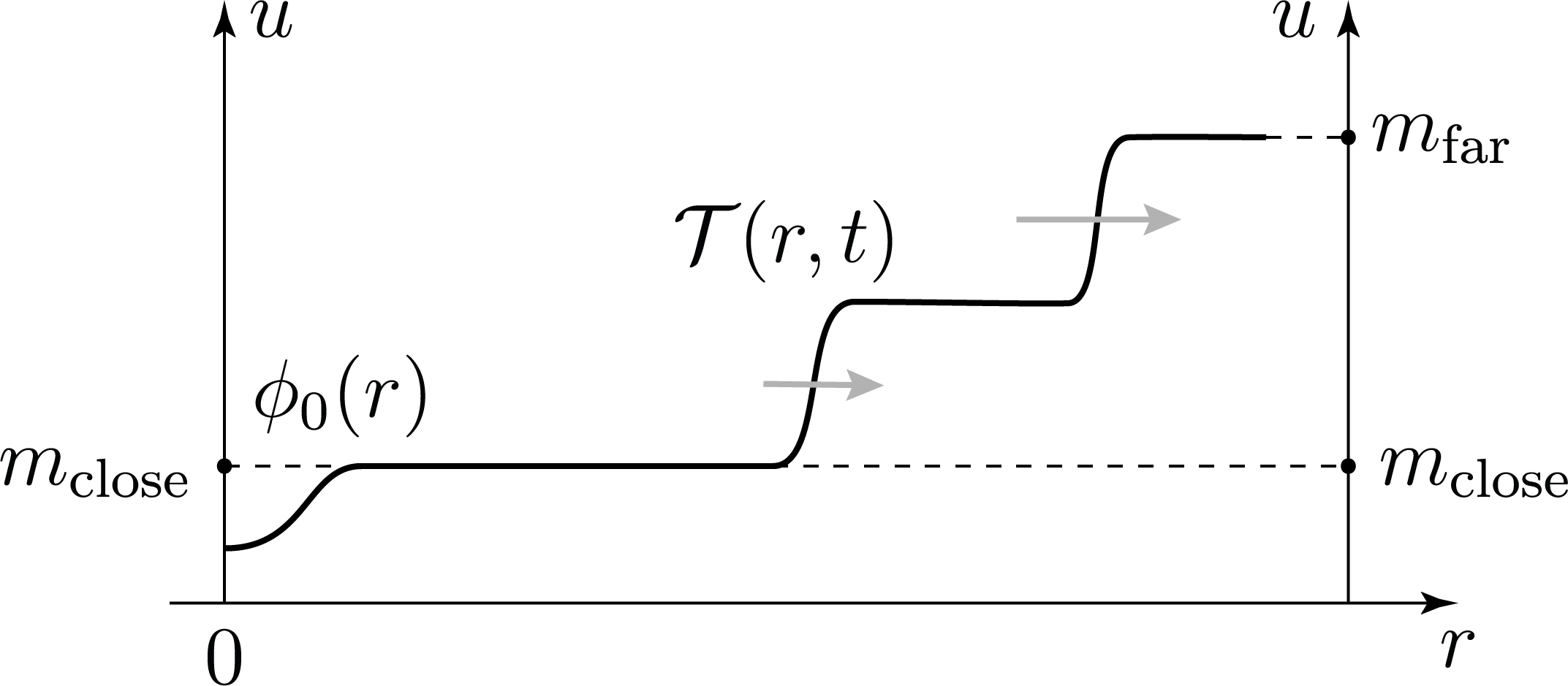
Figure 2.2: Asymptotic pattern stable at infinity.

Definition 2.4 (asymptotic pattern stable at infinity, figure 2.2).

Let $m_{\textup{\text{far}}}$ be a point of $\mathcal{M}$. A function

$$\mathcal{P}:[0,+\infty)\times[0,+\infty)\to\mathbb{R}^{{d_{\textup{\text{st}}}}},\quad(r,t)\mapsto\mathcal{P}(r,t)$$

is called an asymptotic pattern stable close to $m_{\textup{\text{far}}}$ at infinity if there exists:

• a point $m_{\textup{\text{close}}}$ in $\mathcal{M}$,

• and a propagating terrace $\mathcal{T}$ of bistable fronts travelling to the right, connecting $m_{\textup{\text{close}}}$ to $m_{\textup{\text{far}}}$,

• and a stationary solution $\phi_{0}$ in $\Phi_{0,\textup{\text{centre}}}(m_{\textup{\text{close}}})$,

such that, for every nonnegative quantity $r$ and for every nonnegative time $t$,

$$\mathcal{P}(r,t)=\phi_{0}(r)+\bigl{(}\mathcal{T}(r,t)-m_{\textup{\text{close}}}\bigr{)}\,.$$

2.4 Generic hypotheses on the potential

2.4.1 Escape distance of a minimum point

Notation.

For every $u$ in $\mathbb{R}^{d}$, let $\sigma\bigl{(}D^{2}V(u)\bigr{)}$ denote the spectrum (the set of eigenvalues) of the Hessian matrix of $V$ at $u$, and let $\lambda_{\min}(u)$ denote the minimum of this spectrum:

(2.7) $$\lambda_{\min}(u)=\min\Bigl{(}\sigma\bigl{(}D^{2}V(u)\bigr{)}\Bigr{)}\,.$$

Definition 2.5 (Escape distance of a nondegenerate minimum point).

For every $m$ in $\mathcal{M}$, let us call Escape distance of $m$, and let us denote by $\delta_{\textup{\text{Esc}}}(m)$, the supremum of the set

(2.8) $$\Bigl{\{}\delta\in[0,1]:\text{ for all }u\text{ in }\mathbb{R}^{d}\text{ satisfying }\left\lvert u-m\right\rvert_{\mathcal{D}}\leq\delta,\quad\lambda_{\min}(u)\geq\frac{1}{2}\lambda_{\min}(m)\Bigr{\}}\,.$$

Since the quantity $\lambda_{\min}(u)$ varies continuously with $u$, this Escape distance $\delta_{\textup{\text{Esc}}}(m)$ is positive (thus in $(0,1]$). In addition, for all $u$ in $\mathbb{R}^{d}$ such that $\left\lvert u-m\right\rvert_{\mathcal{D}}$ is not larger than $\delta_{\textup{\text{Esc}}}(m)$, the following inequality holds:

(2.9) $$\lambda_{\min}(u)\geq\frac{1}{2}\lambda_{\min}(m)\,.$$

Remark.

This notation $\delta_{\textup{\text{Esc}}}(m)$ refers to the word “distance” (and “Escape”) and should not be mingled with the space dimension $d$.

2.4.2 Breakup of space translation invariance for travelling fronts

For every ordered pair $(m_{-},m_{+})$ of points of $\mathcal{M}$, every positive quantity $c$, and every function $\phi$ in $\Phi_{c}(m_{-},m_{+})$,

$$\sup_{\rho\in\mathbb{R}}\left\lvert\phi(\rho)-m_{-}\right\rvert>\delta_{\textup{\text{Esc}}}(m_{-})\quad\text{and}\quad\sup_{\rho\in\mathbb{R}}\left\lvert\phi(\rho)-m_{+}\right\rvert>\delta_{\textup{\text{Esc}}}(m_{+})\,,$$

see figure 2.3. For a proof of this standard result, see for instance [54, Lemma 7.1].

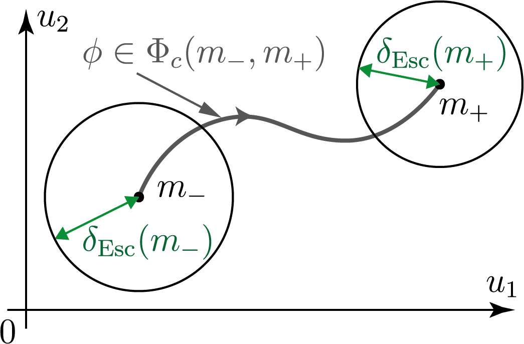
Figure 2.3: Every function in $\Phi_{c}(m_{-},m_{+})$ escapes at least at distance $\delta_{\textup{\text{Esc}}}(m_{-})$ of $m_{-}$ and at distance $\delta_{\textup{\text{Esc}}}(m_{+})$ of $m_{+}$.

Thus, for every positive quantity $c$ and every ordered pair $(m_{-},m_{+})$ of points of $\mathcal{M}$, let us introduce the set of normalized bistable fronts (travelling at the speed $c$) connecting $m_{-}$ to $m_{+}$, defined as

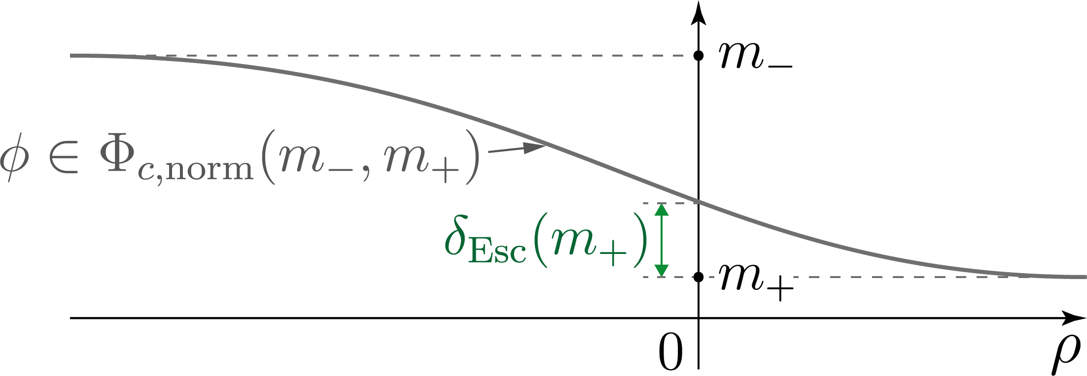
Figure 2.4: Normalized bistable travelling front.

(2.10) $$\Phi_{c,\textup{\text{norm}}}(m_{-},m_{+})=\bigl{\{} \phi\in\Phi_{c}(m_{-},m_{+}):\left\lvert\phi(0)-m_{+}\right\rvert=\delta_{\textup{\text{Esc}}}(m_{+})\quad\text{and}$$

$$\left\lvert\phi(\rho)-m_{+}\right\rvert<\delta_{\textup{\text{Esc}}}(m_{+})\quad\text{for every positive quantity }\rho\bigr{\}}\,,$$

see figure 2.4.

2.4.3 Statement of the generic hypotheses

The results of this paper require a number of generic hypotheses on the potential $V$, that will now be stated.

Notation.

If $m_{+}$ is a point in $\mathcal{M}$ and $c$ is a positive quantity, let $\Phi_{c}(m_{+})$ denote the set of bounded (thus globally defined) profiles of nonconstant waves travelling at the speed $c$ and “invading” the homogeneous equilibrium $m_{+}$; with symbols,

$$\Phi_{c}(m_{+})=\bigl{\{} \phi:\mathbb{R}\to\mathbb{R}^{d}:\phi\text{ is a \emph{nonconstant} global solution of system \lx@cref{creftype~refnum}{syst_trav_front}}$$

$$\text{and}\quad\sup_{\rho\in\mathbb{R}}\left\lvert\phi(\rho)\right\rvert<+\infty\quad\text{and}\quad\phi(\rho)\xrightarrow[\rho\to+\infty]{}m_{+}\bigr{\}}\,,$$

and let

$$\Phi_{c,\textup{\text{norm}}}(m_{+})=\bigl{\{} \phi\in\Phi_{c}(m_{+}):\left\lvert\phi(0)-m_{+}\right\rvert=\delta_{\textup{\text{Esc}}}(m_{+})\quad\text{and}$$

$$\left\lvert\phi(\rho)-m_{+}\right\rvert<\delta_{\textup{\text{Esc}}}(m_{+})\quad\text{for all}\quad\rho\text{ in }(0,+\infty)\bigr{\}}\,.$$

Here are the six generic hypotheses that will be required.

$\textup{\text{(H}}_{\textup{\text{only-bist}}}\textup{\text{)}}$

Every nonconstant bounded wave travelling at a nonzero speed and invading a stable equilibrium (a point of $\mathcal{M}$) is a bistable travelling front. With symbols, for every $m_{+}$ in $\mathcal{M}$ and every positive quantity $c$,

$$\Phi_{c}(m_{+}) =\bigcup_{m_{-}\in\mathcal{M}}\Phi_{c}(m_{-},m_{+})\,,$$

$$\text{or equivalently}\quad\Phi_{c,\textup{\text{norm}}}(m_{+}) =\bigcup_{m_{-}\in\mathcal{M}}\Phi_{c,\textup{\text{norm}}}(m_{-},m_{+})\,.$$

$\textup{\text{(H}}_{\textup{\text{disc-}}c}\textup{\text{)}}$

For every $m_{+}$ in $\mathcal{M}$, the set:

$$\bigl{\{}c\text{ in }[0,+\infty):\Phi_{c}(m_{+})\not=\emptyset\bigr{\}}$$

has an empty interior.

$\textup{\text{(H}}_{\textup{\text{disc-}}\Phi}\textup{\text{)}}$

For every point $m_{+}$ in $\mathcal{M}$ and every positive quantity $c$, the set

$$\bigl{\{}\bigl{(}\phi(0),\phi^{\prime}(0)\bigr{)}:\phi\in\Phi_{c,\textup{\text{norm}}}(m_{+})\bigr{\}}$$

is totally discontinuous — if not empty — in $\mathbb{R}^{2{d_{\textup{\text{st}}}}}$. That is, its connected components are singletons. Equivalently, the set $\Phi_{c,\textup{\text{norm}}}(m_{+})$ is totally disconnected for the topology of compact convergence (uniform convergence on compact subsets of $\mathbb{R}$).

In these two last definitions, the subscript “disc” refers to the concept of “discontinuity” or “discreteness”. The following hypothesis will be required to ensure that the number of travelling fronts involved in the asymptotic behaviour of a radially symmetric solution stable at infinity is finite:

$\textup{\text{(H}}_{\textup{\text{crit-val}}}\textup{\text{)}}$

The set of critical values of $V$, that is the set

$$\bigl{\{}V(u):u\in\mathbb{R}^{d}\text{ and }\nabla V(u)=0\bigr{\}}\,,$$

is finite.

The next hypothesis is the analogue of ($\textup{\text{H}}_{\textup{\text{disc-}}\Phi}$) for radially symmetric stationary solutions.

$\textup{\text{(H}}_{\textup{\text{disc-stat}}}\textup{\text{)}}$

For every point $m$ in $\mathcal{M}$, the set

$$\bigl{\{}\phi(0):\phi\in\Phi_{0,\textup{\text{centre}}}(m)\bigr{\}}$$

is totally discontinuous in $\mathbb{R}^{{d_{\textup{\text{st}}}}}$. That is, its connected components are singletons. Equivalently, the set $\Phi_{0,\textup{\text{centre}}}(m)$ is totally disconnected for the topology of compact convergence (uniform convergence on compact subsets of $[0,+\infty)$).

Finally, let us us call G the union of these five generic hypotheses:

(G) $$\text{{{}(\hyperlink{hypOnlyBist}{$\textup{\text{H}}_{\textup{\text{only-bist}}}$})} and {{}(\hyperlink{hypDiscVel}{$\textup{\text{H}}_{\textup{\text{disc-}}c}$})} and {{}(\hyperlink{hypDiscFront}{$\textup{\text{H}}_{\textup{\text{disc-}}\Phi}$})} and {{}(\hyperlink{hypCriticalValues}{$\textup{\text{H}}_{\textup{\text{crit-val}}}$})} and {{}(\hyperlink{hypDiscStationary}{$\textup{\text{H}}_{\textup{\text{disc-stat}}}$})}}.$$

A formal proof of the genericity of these hypotheses is provided in [27] (for ($\textup{\text{H}}_{\textup{\text{only-bist}}}$), ($\textup{\text{H}}_{\textup{\text{disc-}}c}$), ($\textup{\text{H}}_{\textup{\text{disc-}}\Phi}$), and ($\textup{\text{H}}_{\textup{\text{crit-val}}}$)) and in [53] (for ($\textup{\text{H}}_{\textup{\text{disc-stat}}}$)).

2.5 Main result

Theorem 1 (global asymptotic behaviour).

Let $V$ denote a function in $\mathcal{C}^{2}(\mathbb{R}^{{d_{\textup{\text{st}}}}},\mathbb{R})$ satisfying the coercivity hypothesis $\text{H}_{\text{coerc}}$ and the generic hypotheses G. Then, for every solution stable at infinity $(r,t)\mapsto u(r,t)$ of system 1.2, there exists an asymptotic pattern $\mathcal{P}$ stable at infinity such that

$$\sup_{r\in[0,+\infty)}\left\lvert u(r,t)-\mathcal{P}(r,t)\right\rvert\to 0\quad\text{as}\quad t\to+\infty\,.$$

2.6 Additional results

2.6.1 Residual asymptotic energy

Here is an additional conclusion to Theorem 1.

Proposition 2.6 (residual asymptotic energy).

Assume that the assumptions of Theorem 1 hold. With the notation of this theorem, if $m_{\textup{\text{close}}}$ and $m_{\textup{\text{far}}}$ denote the two points of $\mathcal{M}$ such that the propagating terrace $\mathcal{T}$ involved in the asymptotic pattern of the solution connects $m_{\textup{\text{close}}}$ to $m_{\textup{\text{far}}}$, and if $\phi_{0}$ denotes the function of $\Phi_{0,\textup{\text{centre}}}(m_{\textup{\text{close}}})$ involved in this asymptotic pattern, then, for every small enough positive quantity $\varepsilon$,

$$\int_{0}^{\varepsilon t}r^{d-1}\Bigl{(}\frac{1}{2}u_{r}(r,t)^{2}+V\bigl{(}u(r,t)\bigr{)}-V(m_{\textup{\text{close}}})\Bigr{)}\,dr\to\mathcal{E}[\phi_{0}]\quad\text{as}\quad t\to+\infty\,.$$

The quantity $\mathcal{E}[\phi_{0}]$ may be called the residual asymptotic energy of the solution.

2.6.2 “Mountain pass” existence of a “ground state”

Assume that $V$ satisfies hypothesis $\text{H}_{\text{coerc}}$.

Notation.

If $m$ is a point in $\mathcal{M}$, let $\mathcal{B}_{\textup{\text{att}}}(m)$ denote the basin of attraction (for the semi-flow of system 1.2) of the homogeneous equilibrium $m$:

$$\mathcal{B}_{\textup{\text{att}}}(m)=\bigl{\{}u_{0}\in Y:(S_{t}u_{0})(r)\to m\text{ , uniformly with respect to }r,\text{ as }t\to+\infty\bigr{\}}\,,$$

and let $\partial\mathcal{B}_{\textup{\text{att}}}(m)$ denote the topological border, in $Y$, of $\mathcal{B}_{\textup{\text{att}}}(m)$.

The following statement can be seen as the “semi-flow” version of a standard result ensuring the existence of a “ground state” for system 2.1. Variants of this existence result have been established in numerous references, for instance in [5] (by a direct “shooting” method probably specific to the scalar case where ${d_{\textup{\text{st}}}}$ is equal to $1$), and in [4] (by a more general variational method).

Proposition 2.7 (“mountain pass” existence of a “ground state” and attractor of the border of the basin of attraction of a stable homogeneous equilibrium).

Assume that $V$ satisfies hypothesis $\text{H}_{\text{coerc}}$ and let $m$ be a point in $\mathcal{M}$ which is not a global minimum point of $V$. Then the following conclusions hold.

1. There exists at least one nonconstant function in $\Phi_{0,\textup{\text{centre}}}(m)$.

2. The set $\partial\mathcal{B}_{\textup{\text{att}}}(m)\cap Y_{\textup{\text{stab-infty}}}(m)$ is nonempty.

3. For every solution $(r,t)\mapsto u(r,t)$ of system 1.2 in this set $\partial\mathcal{B}_{\textup{\text{att}}}(m)\cap Y_{\textup{\text{stab-infty}}}(m)$, there exists a function $\phi$ in $\Phi_{0,\textup{\text{centre}}}(m)$ such that $\phi$ is not identically equal to $m$ and such that

   $$\left\lvert u(r,t)-\phi(r)\right\rvert\to 0\quad\text{as}\quad t\to+\infty\,,$$

   uniformly with respect to $r$ in $[0,+\infty)$.

3 Preliminaries

As everywhere else, let us consider a function $V$ in $\mathcal{C}^{2}(\mathbb{R}^{{d_{\textup{\text{st}}}}},\mathbb{R})$ satisfying the coercivity hypothesis $\text{H}_{\text{coerc}}$.

3.1 Global existence of solutions and attracting ball for the semi-flow

Proposition 3.1 (global existence of solutions and attracting ball).

For every function $u_{0}$ in $Y$, system 1.2 has a unique globally defined solution $t\mapsto S_{t}u_{0}$ in $\mathcal{C}^{0}([0,+\infty),Y)$ with initial condition $u_{0}$. In addition, there exist a positive quantity $R_{\textup{\text{att}},\infty}$ (radius of attracting ball for the $L^{\infty}$-norm), depending only on $V$, such that, for every large enough positive time $t$,

$$\left\lVert r\mapsto(S_{t}u_{0})(r)\right\rVert_{L^{\infty}\bigl{(}[0,+\infty),\mathbb{R}^{{d_{\textup{\text{st}}}}}\bigr{)}} \leq R_{\textup{\text{att}},\infty}\,,$$

$$\text{and}\qquad\left\lVert r\mapsto(S_{t}u_{0})(r)\right\rVert_{H^{1}_{\textup{\text{ul}}}\bigl{(}[0,+\infty),\mathbb{R}^{{d_{\textup{\text{st}}}}}\bigr{)}} \leq R_{\textup{\text{att}},1,\textup{\text{ul}}}\,.$$

Proof.

For a proof of this rather standard result, see for instance [56, Proposition 3.1], which provides identical conclusions for system 1.1 (without the radial symmetry hypothesis). ∎

In addition, system 1.2 has smoothing properties (Henry [26]). Due to these properties, since $V$ is of class $\mathcal{C}^{2}$, for every quantity $\alpha$ in the interval $(0,1)$, every solution $t\mapsto S_{t}u_{0}$ in $\mathcal{C}^{0}([0,+\infty),Y)$ actually belongs to

$$\mathcal{C}^{0}\left((0,+\infty),\mathcal{C}^{2,\alpha}_{\textup{\text{b}}}\bigl{(}[0,+\infty),\mathbb{R}^{{d_{\textup{\text{st}}}}}\bigr{)}\right)\cap\mathcal{C}^{1}\left((0,+\infty),\mathcal{C}^{0,\alpha}_{\textup{\text{b}}}\bigl{(}[0,+\infty),\mathbb{R}^{{d_{\textup{\text{st}}}}}\bigr{)}\right),$$

and, for every positive quantity $\varepsilon$, the quantities

(3.1) $$\sup_{t\geq\varepsilon}\left\lVert S_{t}u_{0}\right\rVert_{\mathcal{C}^{2,\alpha}_{\textup{\text{b}}}\bigl{(}[0,+\infty),\mathbb{R}^{{d_{\textup{\text{st}}}}}\bigr{)}}\quad\text{and}\quad\sup_{t\geq\varepsilon}\left\lVert\frac{d(S_{t}u_{0})}{dt}(t)\right\rVert_{\mathcal{C}^{0,\alpha}_{\textup{\text{b}}}\bigl{(}[0,+\infty),\mathbb{R}^{{d_{\textup{\text{st}}}}}\bigr{)}}$$

are finite.

3.2 Asymptotic compactness of solutions

The next two lemmas will be used in the proofs of Propositions 4.1 and 6.1.

Lemma 3.2 (asymptotic compactness in the infinite radius limit).

For every solution $(r,t)\mapsto u(r,t)$ of system 1.2, and for every sequence $(r_{n},t_{n})_{n\in\mathbb{N}}$ in $[0,+\infty)^{2}$ such that $r_{n}$ and $t_{n}$ go to $+\infty$ as $n$ goes to $+\infty$, there exists a entire solution $\macc@depth\char 1\relax\frozen@everymath{\macc@group}\macc@set@skewchar\macc@nested@a 111{u}$ of system 2.4 in

$$\mathcal{C}^{0}\left(\mathbb{R},\mathcal{C}^{2}_{\textup{\text{b}}}\bigl{(}\mathbb{R},\mathbb{R}^{{d_{\textup{\text{st}}}}}\bigr{)}\right)\cap\mathcal{C}^{1}\left(\mathbb{R},\mathcal{C}^{0}_{\textup{\text{b}}}\bigl{(}\mathbb{R},\mathbb{R}^{{d_{\textup{\text{st}}}}}\bigr{)}\right)\,,$$

such that, up to replacing the sequence $(r_{n},t_{n})_{n\in\mathbb{N}}$ by a subsequence,

(3.2) $$D^{2,1}u(r_{n}+\cdot,t_{n}+\cdot)\to D^{2,1}\macc@depth\char 1\relax\frozen@everymath{\macc@group}\macc@set@skewchar\macc@nested@a 111{u}\quad\text{as}\quad n\to+\infty\,,$$

uniformly on every compact subset of $\mathbb{R}^{2}$, where the symbol $D^{2,1}v$ stands for $(v,v_{r},v_{rr},v_{t})$ (for $v$ equal to $u$ or $\macc@depth\char 1\relax\frozen@everymath{\macc@group}\macc@set@skewchar\macc@nested@a 111{u}$).

Lemma 3.3 (asymptotic compactness close to the origin).

For every solution $(r,t)\mapsto u(r,t)$ of system 1.2, and for every sequence $(t_{n})_{n\in\mathbb{N}}$ in $[0,+\infty)$ such that $t_{n}\to+\infty$ as $n\to+\infty$, there exists a entire solution $\macc@depth\char 1\relax\frozen@everymath{\macc@group}\macc@set@skewchar\macc@nested@a 111{u}$ of system 1.2 in

$$\mathcal{C}^{0}\left(\mathbb{R},\mathcal{C}^{2}_{\textup{\text{b}}}\bigl{(}[0,+\infty),\mathbb{R}^{{d_{\textup{\text{st}}}}}\bigr{)}\right)\cap\mathcal{C}^{1}\left(\mathbb{R},\mathcal{C}^{0}_{\textup{\text{b}}}\bigl{(}[0,+\infty),\mathbb{R}^{{d_{\textup{\text{st}}}}}\bigr{)}\right)\,,$$

such that, up to replacing the sequence $(t_{n})_{n\in\mathbb{N}}$ by a subsequence,

(3.3) $$D^{2,1}u(x_{n}+\cdot,t_{n}+\cdot)\to D^{2,1}\macc@depth\char 1\relax\frozen@everymath{\macc@group}\macc@set@skewchar\macc@nested@a 111{u}\quad\text{as}\quad n\to+\infty\,,$$

uniformly on every compact subset of $[0,+\infty)\times\mathbb{R}$

Proofs of Lemmas 3.2 and 3.3.

See [32, 1963] or the proof of [57, Lemma 3.2]. ∎

3.3 Time derivative of (localized) energy and $L^{2}$-norm of a solution

Let $(r,t)\mapsto u(r,t)$ be a solution of system 1.2 and $m$ be a point of $\mathcal{M}$. Let us assume, in the next calculations, that $t$ is positive, so that according to 3.1 the regularities of $u$ and $u_{t}$ ensure that all integrals converge.

3.3.1 Standing frame

Let $r\mapsto\psi(r)$ denote a function in the space $W^{1,1}\bigl{(}[0,+\infty),\mathbb{R}\bigr{)}$ (that is a function belonging to $L^{1}\bigl{(}[0,+\infty)\bigr{)}$ together with its first derivative), and let us introduce the energy (Lagrangian) and the $L^{2}$-norm of the distance to $m$, localized by the weight function $\psi$:

$$\int_{0}^{+\infty}\psi(r)\Bigl{(}\frac{1}{2}u_{r}(r,t)^{2}+V\bigl{(}u(r,t)-V(m)\bigr{)}\Bigr{)}\,dr\quad\text{and}\quad\int_{0}^{+\infty}\psi(r)\frac{1}{2}\bigl{(}u(r,t)-m\bigr{)}^{2}\,dr\,.$$

Let us assume that $\psi(0)=0$, and, to simplify the presentation, let us assume that

$$m=0_{\mathbb{R}^{{d_{\textup{\text{st}}}}}}\quad\text{and}\quad V(m)=V(0_{\mathbb{R}^{{d_{\textup{\text{st}}}}}})=0\,.$$

Then the time derivatives of the two integrals above read:

(3.4) $$\frac{d}{dt}\int_{0}^{+\infty}\psi\Bigl{(}\frac{1}{2}u_{r}^{2}+V(u)\Bigr{)}\,dr=\int_{0}^{+\infty}\biggl{[}-\psi u_{t}^{2}+\Bigl{(}\frac{d-1}{r}\psi-\psi^{\prime}\Bigl{)}u_{t}\cdot u_{r}\biggr{]}\,dr\,,$$

and

(3.5) $$\frac{d}{dt}\int_{0}^{+\infty}\psi\frac{1}{2}u^{2}\,dr=\int_{0}^{+\infty}\biggl{[}\psi\bigl{(}-u\cdot\nabla V(u)-u_{r}^{2}\bigr{)}+\Bigl{(}\frac{d-1}{r}\psi-\psi^{\prime}\Bigl{)}u\cdot u_{r}\biggr{]}\,dr\,.$$

In both expressions, the border term at $r$ equals $0$ coming from the integration by parts vanishes since $\psi(0)=0$. In both expressions again, the last term disappears on every domain where $\psi(r)$ is proportional to $r^{d-1}$ (this corresponds to a uniform weight for the Lebesgue measure on $\mathbb{R}^{d}$).

More comments on these expressions are provided in [57]. The sole difference with the one-dimensional space case treated in [57] is the “$(d-1)/r$” curvature terms on the right-hand side of these expressions. Fortunately, this additional term will not induce many changes with respect to the arguments developed in [57], since:

• close to the origin $r=0$, the weight function $\psi$ can be chosen proportional to $r^{d-1}$,

• far away from the origin $r=0$, this curvature term is just small.

3.3.2 Travelling frame

Now let us introduce nonnegative quantities $c$ and $t_{\textup{\text{init}}}$ and $r_{\textup{\text{init}}}$ (the speed, origin of time, and initial origin of space for the travelling frame respectively, see 4.8). For every nonnegative quantity $s$, let us introduce the interval:

$$I(s)=[-r_{\textup{\text{init}}}-cs,+\infty)\,,$$

and, for every $\rho$ in $I(s)$, let

$$v(\rho,s)=u(r,t)\quad\text{where}\quad r=r_{\textup{\text{init}}}+cs+\rho\quad\text{and}\quad t=t_{\textup{\text{init}}}+s$$

denote the same solution viewed in a referential travelling at the speed $c$. This function $(\rho,s)\mapsto v(\rho,s)$ is a solution of the system:

$$v_{s}-cv_{\rho}=-\nabla V(v)+\frac{d-1}{r_{\textup{\text{init}}}+cs+\rho}v_{\rho}+v_{\rho\rho}\,.$$

This time, let us assume that the weight function $\psi$ is a function of the two variables $\rho$ and $s$, defined on the domain

$$\bigl{\{}(\rho,s)\in\mathbb{R}\times[0,+\infty):\rho\in I(s)\bigr{\}}$$

and such that, for all $s$ in $[0,+\infty)$, the function $\rho\mapsto\psi(\rho,s)$ belongs to $W^{2,1}\bigl{(}I(s),\mathbb{R}\bigr{)}$ and the time derivative $\rho\mapsto\psi_{s}(\rho,s)$ is defined and belongs to $L^{1}\bigl{(}I(s),\mathbb{R}\bigr{)}$. Again, let us introduce the energy (Lagrangian) and the $L^{2}$-norm of the solution, localized by the weight function $\psi$:

$$\int_{I(s)}\psi(\rho,s)\Bigl{(}\frac{1}{2}v_{\rho}(\rho,s)^{2}+V\bigl{(}v(\rho,s)\bigr{)}\Bigr{)}\,d\rho\quad\text{and}\quad\int_{I(s)}\psi(\rho,s)\frac{1}{2}v(\rho,s)^{2}\,d\rho\,.$$

Let us assume in addition that, for all $s$ in $[-t_{\textup{\text{init}}},+\infty)$, the functions $\rho\mapsto\psi(\rho,s)$ and $\rho\mapsto\psi_{\rho}(\rho,s)$ vanish at $\rho=-r_{\textup{\text{init}}}-cs$ (at the left end of its domain of definition). Then the time derivatives of these two quantities read:

(3.6) $$\frac{d}{ds}\int_{I(s)}\psi\Bigl{(}\frac{1}{2}v_{\rho}^{2}+V(v)\Bigr{)}\,d\rho= \int_{I(s)}\biggl{[}-\psi v_{s}^{2}+\psi_{s}\Bigl{(}\frac{1}{2}v_{\rho}^{2}+V(v)\Bigr{)}$$

$$+\Bigl{(}\frac{d-1}{r_{\textup{\text{init}}}+cs+\rho}\psi+c\psi-\psi_{\rho}\Bigl{)}v_{s}\cdot v_{\rho}\biggr{]}\,d\rho\,,$$

and

(3.7) $$\frac{d}{ds}\int_{I(s)}\psi\frac{1}{2}v^{2}\,d\rho= \int_{I(s)}\biggl{[}\psi\bigl{(}-v\cdot\nabla V(v)-v_{\rho}^{2}\bigr{)}+\psi_{s}\frac{1}{2}v^{2}$$

$$+\Bigl{(}\frac{d-1}{r_{\textup{\text{init}}}+cs+\rho}\psi+c\psi-\psi_{\rho}\Bigl{)}v\cdot v_{\rho}\biggr{]}\,d\rho$$

$$= \int_{I(s)}\biggl{[}\psi\bigl{(}-v\cdot\nabla V(v)-v_{\rho}^{2}\bigr{)}+\frac{\psi_{s}}{2}v^{2}$$

$$+\frac{1}{2}(\psi_{\rho\rho}-c\psi_{\rho})v^{2}+\frac{(d-1)\psi}{r_{\textup{\text{init}}}+cs+\rho}v\cdot v_{\rho}\biggr{]}\,d\rho\,.$$

In these expressions again, the integration by part border terms at $\rho=-r_{\textup{\text{init}}}-cs$ vanish, and some terms simplify where the quantity

(3.8) $$\frac{d-1}{r_{\textup{\text{init}}}+cs+\rho}\psi+c\psi-\psi_{\rho}$$

vanishes, that is where $\psi$ is proportional to the expression

$$(r_{\textup{\text{init}}}+cs+\rho)^{d-1}\exp(c\rho)$$

(combining the Lebesgue measure and the exponential weight $\exp(c\rho)$). For the time derivative of the $L^{2}$-functional, a second expression (after integrating by parts the factor $c\psi-\psi_{\rho}$) is given (it is actually this second expression that will turn out to be the most appropriate for the calculations and estimates to come).

More comments on these expressions are provided in [54]. As in the laboratory frame case, the sole difference with the one-dimensional space case treated in [54] is the “$(d-1)/(r_{\textup{\text{init}}}+cs+\rho)$” curvature terms on the right-hand side of these expressions. Fortunately, this additional term does not induce many changes with respect to the arguments of [54], since:

• close to the “origin” $\rho=-r_{\textup{\text{init}}}-cs$, the weight function can be chosen in such a way that the quantity 3.8 (involving this curvature term) vanishes or remains small,

• far away from the origin, this curvature term is just small.

3.4 Miscellanea

3.4.1 Second order estimates for the potential around a minimum point

Lemma 3.4 (second order estimates for the potential around a minimum point).

For every $m$ in $\mathcal{M}$ and every $u$ in $\mathbb{R}^{{d_{\textup{\text{st}}}}}$ satisfying $\left\lvert u-m\right\rvert\leq\delta_{\textup{\text{Esc}}}(m)$, the following estimates hold:

(3.9) $$V(u)-V(m) \geq\frac{\lambda_{\min}(m)}{4}(u-m)^{2}\,,$$

(3.10) $$\text{and}\qquad(u-m)\cdot\nabla Vu) \geq\frac{\lambda_{\min}(m)}{2}(u-m)^{2}\,,$$

(3.11) $$\text{and}\qquad(u-m)\cdot\nabla V(u) \geq V(u)-V(m)\,.$$

Proof.

The three inequalities follow from inequality 2.9 defining $\delta_{\textup{\text{Esc}}}(m)$ and from three variants of Taylor’s Theorem with Lagrange remainder applied to the function $f$ defined on $[0,1]$ by $f(\theta)=V\bigl{(}m+\theta(u-m)\bigr{)}$ (see [57, Lemma 3.3]). ∎

3.4.2 Lower quadratic hulls of the potential at minimum points

As in [57, 54], let

$$q_{\text{low-hull}}=\min_{m\in\mathcal{M}}\ \inf_{u\in\mathbb{R}^{{d_{\textup{\text{st}}}}}\setminus\{m\}}\ \frac{V(u)-V(m)}{(u-m)^{2}}\,,$$

see figure 3.1.

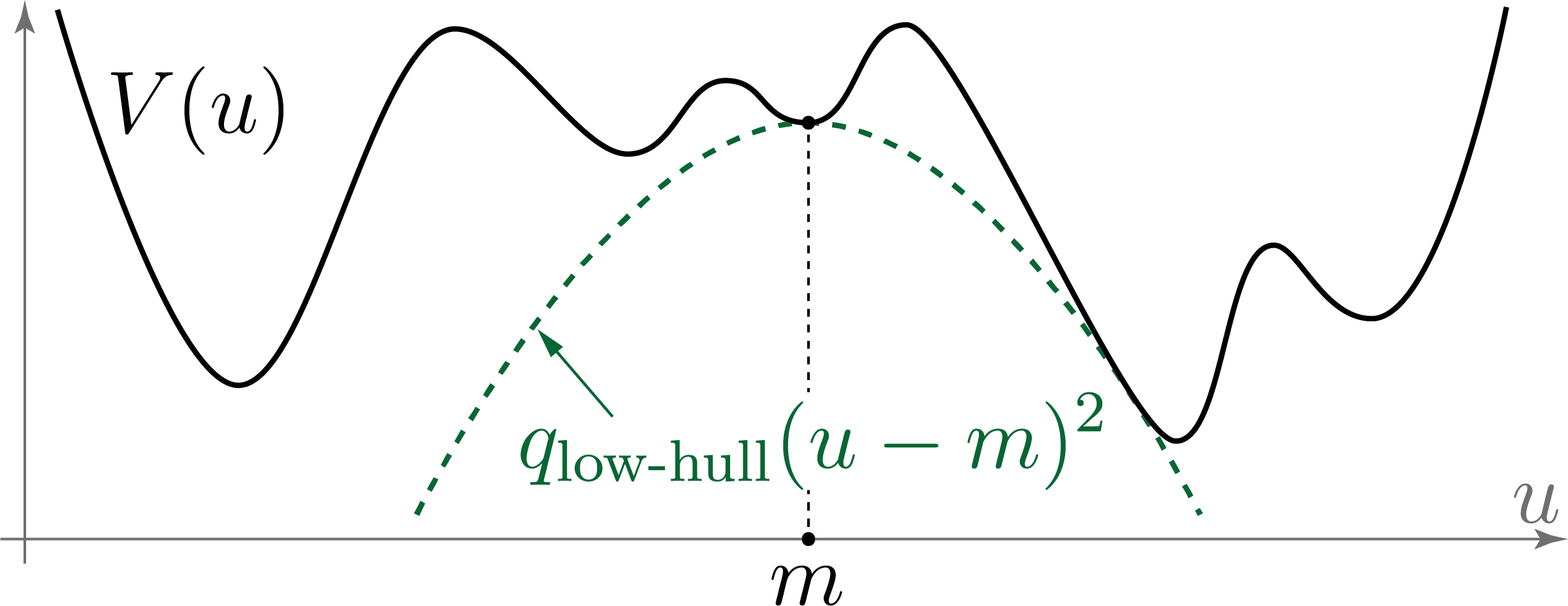
Figure 3.1: Lower quadratic hull of the potential at a minimum point (definition of the quantity $q_{\text{low-hull}}$).

and let

(3.12) $$w_{\textup{\text{en}},0}=\frac{1}{\max(1,-4\,q_{\text{low-hull}})}\,.$$

It follows from this definition that, for every $m$ in the set $\mathcal{M}$ and for all $u$ in $\mathbb{R}^{{d_{\textup{\text{st}}}}}$,

(3.13) $$w_{\textup{\text{en}},0}\,V(u)+\frac{1}{4}(u-m)^{2}\geq 0\,.$$

4 Invasion implies convergence

4.1 Definitions and hypotheses

As everywhere else, let us consider a function $V$ in $\mathcal{C}^{2}(\mathbb{R}^{{d_{\textup{\text{st}}}}},\mathbb{R})$ satisfying the coercivity hypothesis $\text{H}_{\text{coerc}}$. Let us consider a point $m$ in $\mathcal{M}$, a function (initial condition) $u_{0}$ in $Y$, and the corresponding solution $(r,t)\mapsto u(r,t)=(S_{t}u_{0})(r)$ defined on $[0,+\infty)^{2}$.

It will not be assumed that this solution is stable at infinity, but instead, as stated by the next hypothesis ($\textup{\text{H}}_{\textup{\text{hom}}}$), that there exists a growing interval, travelling at a positive speed, where the solution is close to $m$ (the subscript “hom” in the definitions below refers to this “homogeneous” area), see figure 4.1.

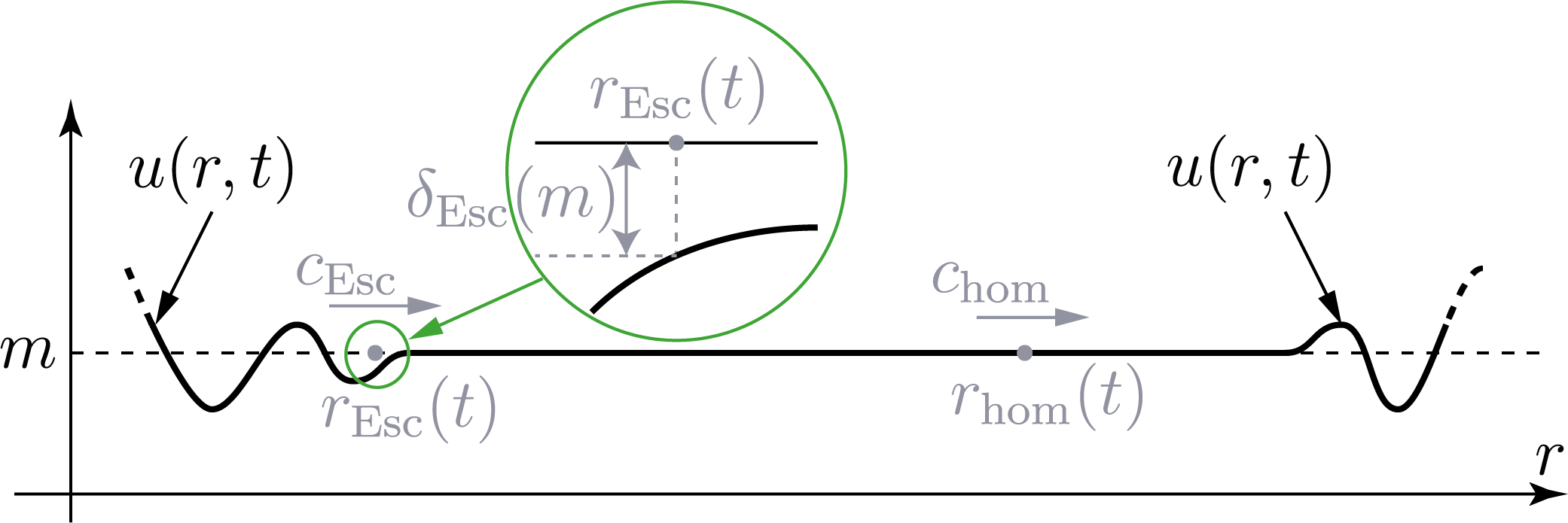
Figure 4.1: Illustration of hypotheses ($\textup{\text{H}}_{\textup{\text{hom}}}$) and ($\textup{\text{H}}_{\textup{\text{inv}}}$).

$\textup{\text{(H}}_{\textup{\text{hom}}}\textup{\text{)}}$

There exists a positive quantity $c_{\textup{\text{hom}}}$ and a $\mathcal{C}^{1}$-function

$$r_{\textup{\text{hom}}}:[0,+\infty)\to\mathbb{R}\,,\quad\text{satisfying}\quad r_{\textup{\text{hom}}}^{\prime}(t)\to c_{\textup{\text{hom}}}\quad\text{as}\quad t\to+\infty\,,$$

such that, for every positive quantity $L$,

$$\sup_{\rho\in[-L,L]}\left\lvert u\bigl{(}r_{\textup{\text{hom}}}(t)+\rho,t\bigr{)}-m\right\rvert\to 0\quad\text{as}\quad t\to+\infty\,.$$

For every $t$ in $[0+\infty)$, let us denote by $r_{\textup{\text{Esc}}}(t)$ the supremum of the set:

$$\Bigl{\{}r\in\bigl{[}0,r_{\textup{\text{hom}}}(t)\bigr{]}:\left\lvert u(r,t)-m\right\rvert=\delta_{\textup{\text{Esc}}}(m)\Bigr{\}}\,,$$

with the convention that $r_{\textup{\text{Esc}}}(t)$ equals $-\infty$ if this set is empty. In other words, $r_{\textup{\text{Esc}}}(t)$ is the first point at the left of $r_{\textup{\text{hom}}}(t)$ where the solution “Escapes” at the distance $r_{\textup{\text{Esc}}}$ from the stable homogeneous equilibrium $m$. This point will be referred to the “Escape point” (with an upper-case “E”, by contrast with another “escape point” that will be introduced later, with a lower-case “e” and a slightly different definition). Let us consider the upper limit of the mean speeds between $0$ and $t$ of this Escape point:

$$c_{\textup{\text{Esc}}}=\limsup_{t\to+\infty}\frac{r_{\textup{\text{Esc}}}(t)}{t}\,,$$

and let us make the following hypothesis, stating that the area around $r_{\textup{\text{hom}}}(t)$ where the solution is close to $m$ is “invaded” from the left at a nonzero (mean) speed.

$\textup{\text{(H}}_{\textup{\text{inv}}}\textup{\text{)}}$

The quantity $c_{\textup{\text{Esc}}}$ is positive.

4.2 Statement

The aim of section 4 is to prove the following proposition, which is the main step in the proof of Theorem 1. The proposition is illustrated by figure 4.2.

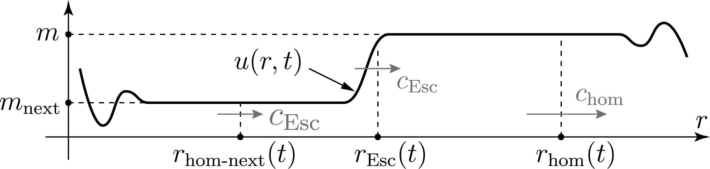
Figure 4.2: Illustration of Proposition 4.1.

Proposition 4.1 (invasion implies convergence).

Assume that $V$ satisfies the coercivity hypothesis $\text{H}_{\text{coerc}}$ and the generic hypotheses ($\textup{\text{H}}_{\textup{\text{only-bist}}}$) and ($\textup{\text{H}}_{\textup{\text{disc-}}c}$) and ($\textup{\text{H}}_{\textup{\text{disc-}}\Phi}$), and, keeping the definitions and notation above, let us assume that for the solution under consideration hypotheses ($\textup{\text{H}}_{\textup{\text{hom}}}$) and ($\textup{\text{H}}_{\textup{\text{inv}}}$) hold. Then the following conclusions hold.

• For $t$ large enough positive, the function $t\mapsto r_{\textup{\text{Esc}}}(t)$ is of class $\mathcal{C}^{1}$ and

  $$r_{\textup{\text{Esc}}}^{\prime}(t)\to c_{\textup{\text{Esc}}}\quad\text{as}\quad t\to+\infty\,.$$

• There exist:

  • a point $m_{\textup{\text{next}}}$ in $\mathcal{M}$ satisfying $V(m_{\textup{\text{next}}})<V(m)$,

  • a profile of travelling front $\phi$ in $\Phi_{c_{\textup{\text{Esc}}},\textup{\text{norm}}}(m_{\textup{\text{next}}},m)$,

  • a $\mathcal{C}^{1}$-function $[0,+\infty)\to\mathbb{R}$, $t\mapsto r_{\textup{\text{hom-next}}}(t)$,

  such that, as time goes to $+\infty$, the following limits hold:

  $$r_{\textup{\text{Esc}}}(t)-r_{\textup{\text{hom-next}}}(t)\to+\infty\quad\text{and}\quad r_{\textup{\text{hom-next}}}^{\prime}(t)\to c_{\textup{\text{Esc}}}$$

  and

  $$\sup_{r\in[r_{\textup{\text{hom-next}}}(t)\,,\ r_{\textup{\text{hom}}}(t)]}\left\lvert u(r,t)-\phi\bigl{(}r-r_{\textup{\text{Esc}}}(t)\bigr{)}\right\rvert\to 0$$

  and, for every positive quantity $L$,

  $$\sup_{\rho\in[-L,L]}\left\lvert u\bigl{(}r_{\textup{\text{hom-next}}}(t)+\rho,t\bigr{)}-m_{\textup{\text{next}}}\right\rvert\to 0\,.$$

4.3 Set-up for the proof, 1

Let us keep the notation and assumptions of subsection 4.1, and let us assume that the hypotheses $\text{H}_{\text{coerc}}$ and ($\textup{\text{H}}_{\textup{\text{only-bist}}}$) and ($\textup{\text{H}}_{\textup{\text{disc-}}c}$) and ($\textup{\text{H}}_{\textup{\text{disc-}}\Phi}$) and ($\textup{\text{H}}_{\textup{\text{hom}}}$) and ($\textup{\text{H}}_{\textup{\text{inv}}}$) of Proposition 4.1 hold.

4.3.1 Assumptions holding up to changing the origin of time

Without loss of generality, up to changing the origin of time, it may be assumed that the following properties hold.

• According to 3.1 (“global existence of solutions and attracting ball”), it may be assumed that, for all $t$ in $[0,+\infty)$,

(4.1) $$\sup_{r\in[0,+\infty)}\,\left\lvert u(r,t)\right\rvert\leq R_{\textup{\text{att}},\infty}\,.$$

• According to the bounds 3.1, it may be assumed that

(4.2) $$\sup_{t\geq 0}\,\left\lVert r\mapsto u(r,t)\right\rVert_{\mathcal{C}^{2}_{\textup{\text{b}}}\bigl{(}[0,+\infty),\mathbb{R}^{{d_{\textup{\text{st}}}}}\bigr{)}} <+\infty$$

$$\text{and}\quad\sup_{t\geq 0}\,\left\lVert r\mapsto u_{t}(r,t)\right\rVert_{\mathcal{C}^{0}_{\textup{\text{b}}}\bigl{(}[0,+\infty),\mathbb{R}^{{d_{\textup{\text{st}}}}}\bigr{)}} <+\infty\,.$$

• According to ($\textup{\text{H}}_{\textup{\text{hom}}}$), it may be assumed that, for all $t$ in $[0,+\infty)$,

(4.3) $$r_{\textup{\text{hom}}}^{\prime}(t)\geq 0\,.$$

4.3.2 Normalized potential and corresponding solution

For notational convenience, let us introduce the “normalized potential” $V^{\dagger}$ and the “normalized solution” $u^{\dagger}$ defined as

(4.4) $$V^{\dagger}(v)=V(m+v)-V(m)\quad\text{and}\quad u^{\dagger}(r,t)=u(r,t)-m\,.$$

Thus the origin $0_{\mathbb{R}^{d}}$ of $\mathbb{R}^{d}$ is to $V^{\dagger}$ what $m$ is to $V$, it is a nondegenerate minimum point for $V^{\dagger}$ (with $V^{\dagger}(0_{\mathbb{R}^{d}})=0$), and $u^{\dagger}$ is a solution of system 1.2 with potential $V^{\dagger}$ instead of $V$; and, for all $(r,t)$ in $[0,+\infty)^{2}$,

$$V^{\dagger}\bigl{(}u^{\dagger}(r,t)\bigr{)}=V\bigl{(}u(r,t)\bigr{)}-V(m)\,.$$

It follows from inequality 3.13 satisfied by $w_{\textup{\text{en}},0}$ that, for all $v$ in $\mathbb{R}^{d}$,

(4.5) $$w_{\textup{\text{en}},0}\,V^{\dagger}(v)+\frac{1}{4}v^{2}\geq 0\,,$$

and it follows from inequalities 3.9, 3.10 and 3.11 that, for all $v$ in $\mathbb{R}^{d}$ satisfying $\left\lvert v\right\rvert\leq\delta_{\textup{\text{Esc}}}(m)$,

(4.6) $$v\cdot\nabla V^{\dagger}(v) \geq\frac{\lambda_{\min}(m)}{2}v^{2}\,,$$

(4.7) $$\text{and}\qquad v\cdot\nabla V^{\dagger}(v) \geq V^{\dagger}(v)\,.$$

4.4 Firewall function in the laboratory frame

4.4.1 Definition

Let $\kappa_{0}$ and $r_{\textup{\text{s-c}}}$ denote two positive quantities, with $\kappa_{0}$ small enough and $r_{\textup{\text{s-c}}}$ large enough so that

(4.8) $$\frac{w_{\textup{\text{en}},0}}{4}\Bigl{(}\frac{d-1}{r_{\textup{\text{s-c}}}}+\kappa_{0}\Bigr{)}^{2}+\frac{1}{4}\Bigl{(}\frac{d-1}{r_{\textup{\text{s-c}}}}+\kappa_{0}\Bigr{)}\leq\frac{1}{2}\quad\text{and}\quad\frac{d-1}{r_{\textup{\text{s-c}}}}+\kappa_{0}\leq\frac{\lambda_{\min}(m)}{8}$$

(those properties will be used to prove inequality 4.20 below). Since according to its definition 3.12 the quantity $w_{\textup{\text{en}},0}$ is not larger than $1$, these quantities may be chosen as

(4.9) $$\kappa_{0}=\min\Bigl{(}\frac{1}{2}\,,\,\frac{\lambda_{\min}(m)}{16}\Bigr{)}$$

and

(4.10) $$r_{\textup{\text{s-c}}}=\max\Bigl{(}2(d-1)\,,\,\frac{16(d-1)}{\lambda_{\min}(m)}\Bigr{)}\,.$$

Let us consider the weight function $\psi_{0}$ defined as

(4.11) $$\psi_{0}(r)=\exp(-\kappa_{0}\left\lvert r\right\rvert)\,,$$

and, for every quantity $\bar{r}$ greater than or equal to $r_{\textup{\text{s-c}}}$, let $T_{\bar{r}}\psi_{0}$ denote the function $[0,+\infty)\to\mathbb{R}$ defined as

(4.12) $$T_{\bar{r}}\psi_{0}(r)=\left\{\begin{aligned} \psi_{0}(r-\bar{r})\Bigl{(}\frac{r}{r_{\textup{\text{s-c}}}}\Bigr{)}^{d-1}&\quad\text{if}\quad 0\leq r\leq r_{\textup{\text{s-c}}}\,,\\ \psi_{0}(r-\bar{r})&\quad\text{if}\quad r\geq r_{\textup{\text{s-c}}}\,,\end{aligned}\right.$$

see figure 4.3.

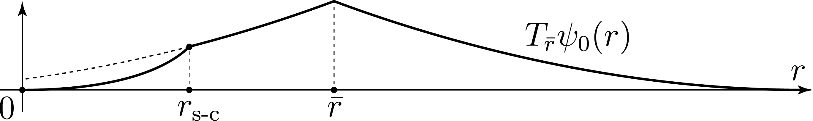
Figure 4.3: Graph of the weight function $r\mapsto T_{\bar{r}}\psi_{0}(r)$ used to define the firewall function $\mathcal{F}_{0}(\bar{r},t)$. The quantity $r_{\textup{\text{s-c}}}$ is large, and, according to the definition of $\kappa_{0}$, the slope is small.

As the following computations will show, for $r$ greater than this quantity $r_{\textup{\text{s-c}}}$, the “curvature terms” that take place in the time derivatives of energy and $L^{2}$ functionals (see expressions LABEL:ddt_loc_en_stand_fr,ddt_loc_L2_stand_fr) will be small enough for the desired estimates to hold. The subscript “s-c” thus refers to “small curvature” (or equivalently, “large radius”).

Thus, the function $T_{\bar{r}}\psi_{0}$ defined above is:

• a translate of the function $\psi_{0}$ far from the origin (for $r$ greater than $r_{\textup{\text{s-c}}}$),

• the same translate multiplied by a factor proportional to the “Lebesgue measure” weight $r^{d-1}$ close to the origin (for $r$ smaller than $r_{\textup{\text{s-c}}}$), this factor being equal to $1$ at $r=r_{\textup{\text{s-c}}}$ to ensure the continuity of the function.

One purpose of this definition is to control the last terms in the expressions 3.4 and 3.5 for the time derivatives of the energy and $L^{2}$ functionals. For all nonnegative quantities $\bar{r}$ and $r$ with $\bar{r}$ not smaller than $r_{\textup{\text{s-c}}}$,

$$\frac{d-1}{r}T_{\bar{r}}\psi_{0}(r)-T_{\bar{r}}\psi_{0}^{\prime}(r)=\left\{\begin{aligned} &-\kappa_{0}T_{\bar{r}}\psi_{0}(r)&&\text{if}\quad r<r_{\textup{\text{s-c}}}\,,\\ &\Bigl{(}\frac{d-1}{r}-\kappa_{0}\Bigr{)}T_{\bar{r}}\psi_{0}(r)&&\text{if}\quad r_{\textup{\text{s-c}}}<r<\bar{r}\,,\\ &\Bigl{(}\frac{d-1}{r}+\kappa_{0}\Bigr{)}T_{\bar{r}}\psi_{0}(r)&&\text{if}\quad\bar{r}<r\,,\\ \end{aligned}\right.$$

thus, in all three cases,

(4.13) $$\left\lvert\frac{d-1}{r}T_{\bar{r}}\psi_{0}(r)-T_{\bar{r}}\psi_{0}^{\prime}(r)\right\rvert\leq\Bigl{(}\frac{d-1}{r_{\textup{\text{s-c}}}}+\kappa_{0}\Bigr{)}T_{\bar{r}}\psi_{0}(r)\,.$$

For all nonnegative quantities $r$ and $t$, let us introduce the quantities

(4.14) $$E^{\dagger}(r,t)=\frac{1}{2}u^{\dagger}_{r}(r,t)^{2}+V^{\dagger}\bigl{(}u^{\dagger}(r,t)\bigr{)}\quad\text{and}\quad F^{\dagger}(r,t)=w_{\textup{\text{en}},0}E^{\dagger}(r,t)+\frac{1}{2}u^{\dagger}(r,t)^{2}\,,$$

and, for all nonnegative quantities $\bar{r}$ and $t$ with $\bar{r}$ not smaller than $r_{\textup{\text{s-c}}}$, let us introduce the “firewall” $\mathcal{F}_{0}(\bar{r},t)$ defined as

(4.15) $$\mathcal{F}_{0}(\bar{r},t)=\int_{0}^{+\infty}T_{\bar{r}}\psi_{0}(r)F^{\dagger}(r,t)\,dr\,.$$

4.4.2 Coercivity

Lemma 4.2 (firewall coercivity).

For every nonnegative time $t$ and nonnegative radius $r$,

(4.16) $$F^{\dagger}(r,t)\geq\min\left(\frac{w_{\textup{\text{en}},0}}{2},\frac{1}{4}\right)\bigl{(}u^{\dagger}_{r}(r,t)^{2}+u^{\dagger}(r,t)^{2}\bigr{)}\,,$$

so that, for every $\bar{r}$ greater than or equal to $r_{\textup{\text{s-c}}}$,

(4.17) $$\mathcal{F}_{0}(\bar{r},t)\geq\min\left(\frac{w_{\textup{\text{en}},0}}{2},\frac{1}{4}\right)\int_{\mathbb{R}}T_{\bar{r}}\psi_{0}(r)\bigl{(}u^{\dagger}_{r}(r,t)^{2}+u^{\dagger}(r,t)^{2}\bigr{)}\,dr\,.$$

Proof.

Inequality 4.16 follows from inequality 4.5 satisfied by $w_{\textup{\text{en}},0}$, and 4.17 follows from 4.16. ∎

4.4.3 Linear decrease up to pollution

For every nonnegative time $t$, let us introduce the following set (the set of radii where the solution “Escapes” at a certain distance from $0_{\mathbb{R}^{{d_{\textup{\text{st}}}}}}$):

(4.18) $$\Sigma_{\textup{\text{Esc}},0}(t)=\bigl{\{}r\in[0,+\infty):\left\lvert u^{\dagger}(r,t)\right\rvert>\delta_{\textup{\text{Esc}}}(m)\bigr{\}}\,,$$

Lemma 4.3 (firewall linear decrease up to pollution).

There exist positive quantities $\nu_{\mathcal{F}_{0}}$ and $K_{\mathcal{F}_{0}}$, depending only on $V$, such that, for all nonnegative quantities $\bar{r}$ and $t$,

(4.19) $$\partial_{t}\mathcal{F}_{0}(\bar{r},t)\leq-\nu_{\mathcal{F}_{0}}\,\mathcal{F}_{0}(\bar{r},t)+K_{\mathcal{F}_{0}}\,\int_{\Sigma_{\textup{\text{Esc}},0}(t)}T_{\bar{r}}\psi_{0}(r)\,dr\,.$$

Proof.

It follows from expressions LABEL:ddt_loc_en_stand_fr,ddt_loc_L2_stand_fr for the time derivatives of localized energy and $L^{2}$-functionals that

$$\partial_{t}\mathcal{F}_{0}(\bar{r},t)= \int_{0}^{+\infty}\biggl{(}T_{\bar{r}}\psi_{0}\bigl{(}-w_{\textup{\text{en}},0}\,(u^{\dagger}_{t})^{2}-u^{\dagger}\cdot\nabla V^{\dagger}(u^{\dagger})-(u^{\dagger}_{r})^{2}\bigr{)}$$

$$+\Bigl{(}\frac{d-1}{r}T_{\bar{r}}\psi_{0}-T_{\bar{r}}\psi_{0}^{\prime}\Bigr{)}\bigl{(}w_{\textup{\text{en}},0}\,u^{\dagger}_{t}\cdot u^{\dagger}_{r}+u^{\dagger}\cdot u^{\dagger}_{r}\bigr{)}\biggr{)}\,dr\,.$$

Thus, according to the upper bound 4.13,

$$\partial_{t}\mathcal{F}_{0}(\bar{r},t) \leq\int_{0}^{+\infty}T_{\bar{r}}\psi_{0}\biggl{(}-w_{\textup{\text{en}},0}\,(u^{\dagger}_{t})^{2}-u^{\dagger}\cdot\nabla V^{\dagger}(u^{\dagger})-(u^{\dagger}_{r})^{2}$$

$$+\left(\frac{d-1}{r_{\textup{\text{s-c}}}}+\kappa_{0}\right)\Bigl{(}w_{\textup{\text{en}},0}\,\left\lvert u^{\dagger}_{t}\cdot u^{\dagger}_{r}\right\rvert+\left\lvert u^{\dagger}\cdot u^{\dagger}_{r}\right\rvert\Bigr{)}\biggr{)}\,dr\,,$$

thus, using the inequalities

$$\left(\frac{d-1}{r_{\textup{\text{s-c}}}}+\kappa_{0}\right)\left\lvert u^{\dagger}_{t}\cdot u^{\dagger}_{r}\right\rvert \leq(u^{\dagger}_{t})^{2}+\frac{1}{4}\left(\frac{d-1}{r_{\textup{\text{s-c}}}}+\kappa_{0}\right)^{2}(u^{\dagger}_{r})^{2}\,,$$

$$\text{and}\quad\left\lvert u^{\dagger}_{t}\cdot u^{\dagger}_{r}\right\rvert \leq\frac{1}{4}(u^{\dagger}_{r})^{2}+(u^{\dagger})^{2}\,,$$

it follows that

$$\partial_{t}\mathcal{F}_{0}(\bar{r},t)\leq \int_{0}^{+\infty}T_{\bar{r}}\psi_{0}\Biggl{[}\biggl{(}\frac{w_{\textup{\text{en}},0}}{4}\Bigl{(}\frac{d-1}{r_{\textup{\text{s-c}}}}+\kappa_{0}\Bigr{)}^{2}+\frac{1}{4}\Bigl{(}\frac{d-1}{r_{\textup{\text{s-c}}}}+\kappa_{0}\Bigr{)}-1\biggr{)}(u^{\dagger}_{r})^{2}$$

$$-u^{\dagger}\cdot\nabla V^{\dagger}(u^{\dagger})+\Bigl{(}\frac{d-1}{r_{\textup{\text{s-c}}}}+\kappa_{0}\Bigr{)}(u^{\dagger})^{2}\Biggr{]}\,dr\,,$$

and according to inequalities 4.8 satisfied by the quantities $\kappa_{0}$ and $r_{\textup{\text{s-c}}}$,

(4.20) $$\partial_{t}\mathcal{F}_{0}(\bar{r},t)\leq\int_{0}^{+\infty}T_{\bar{r}}\psi_{0}\Bigl{(}-\frac{1}{2}(u^{\dagger}_{r})^{2}-u^{\dagger}\cdot\nabla V^{\dagger}(u^{\dagger})+\frac{\lambda_{\min}(m)}{8}(u^{\dagger})^{2}\Bigr{)}\,dr\,.$$

Let $\nu_{\mathcal{F}_{0}}$ be a positive quantity to be chosen below. It follows from the previous inequality and from the definition 4.15 of $\mathcal{F}_{0}(\bar{r},t)$ that

(4.21) $$\partial_{t}\mathcal{F}_{0}(\bar{r},t)+\nu_{\mathcal{F}_{0}}\mathcal{F}_{0}(\bar{r},t)\leq\int_{0}^{+\infty}T_{\bar{r}}\psi_{0}\biggl{[} -\frac{1}{2}(1-\nu_{\mathcal{F}_{0}}\,w_{\textup{\text{en}},0})(u^{\dagger}_{r})^{2}-u^{\dagger}\cdot\nabla V^{\dagger}(u^{\dagger})$$

$$+\nu_{\mathcal{F}_{0}}w_{\textup{\text{en}},0}V^{\dagger}(u^{\dagger})+\Bigl{(}\frac{\lambda_{\min}(m)}{8}+\frac{\nu_{\mathcal{F}_{0}}}{2}\Bigr{)}(u^{\dagger})^{2}\biggr{]}\,dr\,.$$

In view of this inequality and inequalities LABEL:v_nablaV_controls_square_around_loc_min_dag,v_nablaV_controls_pot_around_loc_min_dag, let us assume that $\nu_{\mathcal{F}_{0}}$ is small enough so that

(4.22) $$\nu_{\mathcal{F}_{0}}\,w_{\textup{\text{en}},0}\leq 1\quad\text{and}\quad\nu_{\mathcal{F}_{0}}\,w_{\textup{\text{en}},0}\leq\frac{1}{2}\quad\text{and}\quad\frac{\nu_{\mathcal{F}_{0}}}{2}\leq\frac{\lambda_{\min}(m)}{8}\,;$$

the quantity $\nu_{\mathcal{F}_{0}}$ may be chosen as

(4.23) $$\nu_{\mathcal{F}_{0}}=\min\left(\frac{1}{2w_{\textup{\text{en}},0}},\frac{\lambda_{\min}(m)}{4}\right)\,.$$

Then, it follows from 4.21 and 4.22 that

(4.24) $$\partial_{t}\mathcal{F}_{0}(\bar{r},t)+\nu_{\mathcal{F}_{0}}\mathcal{F}_{0}(\bar{r},t)\leq\int_{0}^{+\infty}T_{\bar{r}}\psi_{0}\Bigl{[}-u^{\dagger}\cdot\nabla V^{\dagger}(u^{\dagger})+\frac{1}{2}\left\lvert V^{\dagger}(u^{\dagger})\right\rvert+\frac{\lambda_{\min}(m)}{4}(u^{\dagger})^{2}\Bigr{]}\,dr\,.$$

According to 4.6 and 4.7, the integrand of the integral at the right-hand side of this inequality is nonpositive as long as $r$ is not in $\Sigma_{\textup{\text{Esc}},0}(t)$. Therefore this inequality still holds if the domain of integration of this integral is changed from $[0,+\infty)$ to $\Sigma_{\textup{\text{Esc}},0}(t)$. Besides, observe that, in terms of the “initial” potential $V$ and solution $u(r,t)$, the factor of $T_{\bar{x}}\psi$ under the integral of the right-hand side of this last inequality reads

$$-(u-m)\cdot\nabla V(u)+\frac{1}{2}\bigl{(}V(u)-V(m)\bigr{)}+\frac{\lambda_{\min}(m)}{4}(u-m)^{2}\,.$$

Thus, if $K_{\mathcal{F}_{0}}$ denotes the maximum of this expression over all possible values for $m$ and $u$, that is the (positive) quantity

(4.25) $$K_{\mathcal{F}_{0}}=\max_{v\in\mathbb{R}^{{d_{\textup{\text{st}}}}},\ \left\lvert v\right\rvert\leq R_{\textup{\text{att}},\infty}}\left[-(u-m)\cdot\nabla V(u)+\frac{1}{2}\left\lvert V(u)-V(m)\right\rvert+\frac{\lambda_{\min}(m)}{4}(u-m)^{2}\right]\,,$$

then inequality 4.19 follows from inequality 4.24 (with the domain of integration of the integral on the right-hand side restricted to $\Sigma_{\textup{\text{Esc}},0}(t)$). Observe that $K_{\mathcal{F}_{0}}$ depends only on $V$. This finishes the proof of Lemma 4.3. ∎

4.5 Upper bound on the invasion speed

Let

(4.26) $$\delta_{\textup{\text{esc}}}(m)=\delta_{\textup{\text{Esc}}}(m)\sqrt{\frac{\min\Bigl{(}\frac{w_{\textup{\text{en}},0}}{2},\frac{1}{4}\Bigr{)}}{\kappa_{0}+1}}\,.$$

As the quantity $\delta_{\textup{\text{Esc}}}(m)$ defined in 2.4.2, this quantity $\delta_{\textup{\text{esc}}}(m)$ will provide a way to measure the vicinity of the solution $u$ to the point $m$, this time in terms of the firewall function $\mathcal{F}_{0}$. The value chosen for $\delta_{\textup{\text{esc}}}(m)$ depends only on $V$ and ensures the validity of the following lemma.

Lemma 4.4 (escape/Escape).

For all $(\bar{r},t)$ in $[r_{\textup{\text{s-c}}},+\infty)\times[0,+\infty)$, the following assertion holds:

(4.27) $$\mathcal{F}_{0}(\bar{r},t)\leq\delta_{\textup{\text{esc}}}(m)^{2}\implies\left\lvert u^{\dagger}(\bar{r},t)\right\rvert\leq\delta_{\textup{\text{Esc}}}(m)\,.$$

Proof.

Let $v$ be a function $Y$, and assume in addition that $v$ is of class $\mathcal{C}^{1}$ and that its derivative is uniformly bounded on $[0,+\infty)$. Then, for all $\bar{r}$ in $[r_{\textup{\text{s-c}}},+\infty)$,

$$v(\bar{r})^{2} =T_{\bar{r}}\psi_{0}(\bar{r})v(\bar{r})^{2}$$

$$\leq\int_{\bar{r}}^{+\infty}\left\lvert\frac{d}{dr}\bigl{(}T_{\bar{r}}\psi_{0}(r)v(r)^{2}\bigr{)}\right\rvert\,dr$$

$$\leq\int_{\bar{r}}^{+\infty}\bigl{(}\left\lvert T_{\bar{r}}\psi_{0}^{\prime}(r)\right\rvert\,v(r)^{2}+2T_{\bar{r}}\psi_{0}(r)\,v(r)\cdot v^{\prime}(r)\bigr{)}\,dr$$

$$\leq\int_{\bar{r}}^{+\infty}T_{\bar{r}}\psi_{0}(r)\bigl{(}(\kappa_{0}+1)v(r)^{2}+v^{\prime}(r)^{2}\bigr{)}\,dr$$

$$\leq(\kappa_{0}+1)\int_{0}^{+\infty}T_{\bar{r}}\psi_{0}(r)\bigl{(}v(r)^{2}+v^{\prime}(r)^{2}\bigr{)}\,dr\,.$$

Thus it follows from inequality 4.17 on the coercivity of $\mathcal{F}_{0}(\cdot,\cdot)$ that, for all $\bar{r}$ in $[r_{\textup{\text{s-c}}},+\infty)$ and $t$ in $[0,+\infty)$,

$$u^{\dagger}(\bar{r},t)^{2}\leq\frac{\kappa_{0}+1}{\min\Bigl{(}\frac{w_{\textup{\text{en}},0}}{2},\frac{1}{4}\Bigr{)}}\mathcal{F}_{0}(\bar{r},t)\,,$$

and this ensures the validity of implication 4.27 with the value of $\delta_{\textup{\text{esc}}}(m)$ chosen in definition 4.26. ∎

Let $L$ be a positive quantity, large enough so that

$$2K_{\mathcal{F}_{0}}\frac{\exp(-\kappa_{0}L)}{\kappa_{0}}\leq\nu_{\mathcal{F}_{0}}\frac{\delta_{\textup{\text{esc}}}(m)^{2}}{8}\,,\quad\text{namely}\quad L=\frac{1}{\kappa_{0}}\log\Bigl{(}\frac{16\,K_{\mathcal{F}_{0}}}{\nu_{\mathcal{F}_{0}}\,\delta_{\textup{\text{esc}}}(m)^{2}\,\kappa_{0}}\Bigr{)}$$

(this quantity depends only on $V$), let $\eta_{\textup{\text{no-esc}}}:\mathbb{R}\to\mathbb{R}\cup\{+\infty\}$ (“no-escape hull”) be the function defined as

(4.28) $$\eta_{\textup{\text{no-esc}}}(\rho)=\left\{\begin{aligned} &+\infty&\quad\text{for}\quad&\rho<0\,,\\ &\frac{\delta_{\textup{\text{esc}}}(m)^{2}}{2}\Bigl{(}1-\frac{\rho}{2\,L}\Bigr{)}&\quad\text{for}\quad&0\leq\rho\leq L\,,\\ &\frac{\delta_{\textup{\text{esc}}}(m)^{2}}{4}&\quad\text{for}\quad&\rho\geq L\,,\end{aligned}\right.$$

Figure 4.4: Graph of the hull function $\eta_{\textup{\text{no-esc}}}$.

see figure 4.4; and let $c_{\textup{\text{no-esc}}}$ (“no-escape speed”) be a positive quantity, large enough so that

$$c_{\textup{\text{no-esc}}}\frac{\delta_{\textup{\text{esc}}}(m)^{2}}{4L}\geq 2\frac{K_{\mathcal{F}_{0}}}{\kappa_{0}}\,,\quad\text{namely}\quad c_{\textup{\text{no-esc}}}=\frac{8\,K_{\mathcal{F}_{0}}\,L}{\kappa_{0}\,\delta_{\textup{\text{esc}}}(m)^{2}}$$

(this quantity depends only on $V$ and $m$). The following lemma, illustrated by figure 4.5, is a variant of [57, Lemma 4.6].

Figure 4.5: Illustration of Lemma 4.5; if the firewall function is below the maximum of two mirror hulls at a certain time $t_{0}$ and if these two hulls travel at opposite speeds $\pm c_{\textup{\text{no-esc}}}$, then the firewall will remain below the maximum of those travelling hulls in the future (note that after they cross this maximum equals $+\infty$ thus the assertion of being “below” is empty).

Lemma 4.5 (bound on invasion speed).

For every ordered pair $(r_{\textup{\text{left}}},r_{\textup{\text{right}}})$ of points in the interval $[r_{\textup{\text{s-c}}},+\infty)$ and every nonnegative time $t_{1}$, if

$$\mathcal{F}_{0}(r,t_{1})\leq\max\bigl{(}\eta_{\textup{\text{no-esc}}}(r-r_{\textup{\text{left}}}),\eta_{\textup{\text{no-esc}}}(r_{\textup{\text{right}}}-r)\bigr{)}\quad\text{for all }r\text{ in }[r_{\textup{\text{s-c}}},+\infty)\,,$$

then, for every time $t$ greater than or equal to $t_{1}$ and all $r$ in $[r_{\textup{\text{s-c}}},+\infty)$,

$$\mathcal{F}_{0}(r,t)\leq\max\Bigl{(}\eta_{\textup{\text{no-esc}}}\bigl{(}r_{\textup{\text{left}}}-c_{\textup{\text{no-esc}}}\,(t-t_{1})\bigr{)},\eta_{\textup{\text{no-esc}}}\bigl{(}r_{\textup{\text{right}}}+c_{\textup{\text{no-esc}}}\,(t-t_{1})-r\bigr{)}\Bigr{)}\,.$$

Proof.

See [57, Lemma 4.6]. ∎

4.6 Set-up for the proof, 2: escape point and associated speeds

According to hypothesis ($\textup{\text{H}}_{\textup{\text{hom}}}$) and to the bounds 4.2 on the solution, it may be assumed, up to changing the origin of time, that, for all $t$ in $[0,+\infty)$ and for all $r$ in $[r_{\textup{\text{s-c}}},+\infty)$,

(4.29) $$r_{\textup{\text{s-c}}} \leq r_{\textup{\text{hom}}}(t)-1\,,$$

$$\text{and}\quad\mathcal{F}_{0}(r,t) \leq\max\biggl{(}\eta_{\textup{\text{no-esc}}}\Bigl{(}r-\bigl{(}r_{\textup{\text{hom}}}(t)-1\bigr{)}\Bigr{)},\eta_{\textup{\text{no-esc}}}\bigl{(}r_{\textup{\text{hom}}}(t)-r\bigr{)}\biggr{)}\,.$$

As a consequence, for all $t$ in $[0,+\infty)$, the set

$$I_{\textup{\text{hom}}}(t)=\Bigl{\{} r_{\ell}\in[r_{\textup{\text{s-c}}},r_{\textup{\text{hom}}}(t)]:\text{ for all }r\text{ in }[r_{\textup{\text{s-c}}},+\infty)\,,$$

$$\mathcal{F}_{0}(r,t)\leq\max\Bigl{(}\eta_{\textup{\text{no-esc}}}(r-r_{\ell}),\eta_{\textup{\text{no-esc}}}\bigl{(}r_{\textup{\text{hom}}}(t)-r\bigr{)}\Bigr{)}\Bigr{\}}$$

is a nonempty interval (containing $[r_{\textup{\text{hom}}}(t)-1,r_{\textup{\text{hom}}}(t)]$), see figure 4.6.

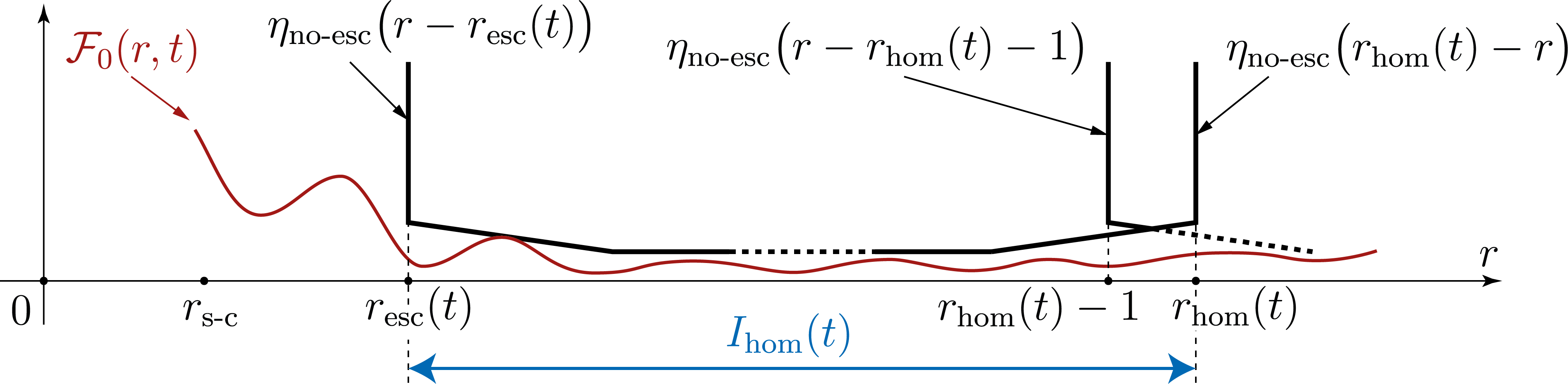
Figure 4.6: Interval $I_{\textup{\text{hom}}}(t)$ and definition of $r_{\textup{\text{esc}}}(t)$.

For all $t$ in $[0,+\infty)$, let

(4.30) $$r_{\textup{\text{esc}}}(t)=\inf\bigl{(}I_{\textup{\text{hom}}}(t)\bigr{)}\quad\text{(thus }r_{\textup{\text{esc}}}(t)\in[r_{\textup{\text{s-c}}},r_{\textup{\text{hom}}}(t)-1]\text{ ).}$$

Somehow like $r_{\textup{\text{Esc}}}(t)$, this point represents the first point at the left of $r_{\textup{\text{hom}}}(t)$ where the solution $u$ (respectively $u^{\dagger}$) “escapes” (in a sense defined by the firewall function $\mathcal{F}_{0}$ and the no-escape hull $\eta_{\textup{\text{no-esc}}}$) at a certain distance from $m$ (respectively from $0_{\mathbb{R}^{{d_{\textup{\text{st}}}}}}$) — except if $I_{\textup{\text{hom}}}(t)$ is the whole interval $[r_{\textup{\text{s-c}}},r_{\textup{\text{hom}}}(t)]$, in this case this “escape” does not occur. In the following, this point $r_{\textup{\text{esc}}}(t)$ will be called the “escape point” (by contrast with the “Escape point” $r_{\textup{\text{Esc}}}(t)$ defined before). According to the “hull inequality” 4.29 and Lemma 4.4 (“escape/Escape”), for all $t$ in $[0,+\infty)$,

(4.31) $$r_{\textup{\text{Esc}}}(t)\leq r_{\textup{\text{esc}}}(t)\leq r_{\textup{\text{hom}}}(t)-1\quad\text{and}\quad\Sigma_{\textup{\text{Esc}},0}(t)\cap[r_{\textup{\text{Esc}}}(t),r_{\textup{\text{hom}}}(t)]=\emptyset\,,$$

and, according to hypothesis ($\textup{\text{H}}_{\textup{\text{hom}}}$) and to the bounds 4.2 on the solution,

(4.32) $$r_{\textup{\text{hom}}}(t)-r_{\textup{\text{esc}}}(t)\to+\infty\quad\text{as}\quad t\to+\infty\,.$$

The big advantage of $r_{\textup{\text{esc}}}(\cdot)$ with respect to $r_{\textup{\text{Esc}}}(\cdot)$ is that, according to Lemma 4.5 (“bound on invasion speed”), the growth of $r_{\textup{\text{esc}}}(\cdot)$ is more under control. More precisely, according to this lemma, for all nonnegative quantities $t$ and $s$,

(4.33) $$r_{\textup{\text{esc}}}(t+s)\leq r_{\textup{\text{esc}}}(t)+c_{\textup{\text{no-esc}}}\,s\,.$$

For every $s$ in $[0,+\infty)$, let us consider the “upper and lower bounds of the variations of $r_{\textup{\text{esc}}}(\cdot)$ over all time intervals of length $s$”:

Figure 4.7: Illustration of the bounds 4.34.

$$\macc@depth\char 1\relax\frozen@everymath{\macc@group}\macc@set@skewchar\macc@nested@a 111{r}_{\textup{\text{esc}}}(s)=\sup_{t\in[0,+\infty)}r_{\textup{\text{esc}}}(t+s)-r_{\textup{\text{esc}}}(t)\quad\text{and}\quad\underline{r}_{\textup{\text{esc}}}(s)=\inf_{t\in[0,+\infty)}r_{\textup{\text{esc}}}(t+s)-r_{\textup{\text{esc}}}(t)\,,$$

see figure 4.7. According to these definitions and to inequality 4.33 above, for all $t$ and $s$ in $[0,+\infty)$,

(4.34) $$-\infty\leq\underline{r}_{\textup{\text{esc}}}(s)\leq r_{\textup{\text{esc}}}(t+s)-r_{\textup{\text{esc}}}(t)\leq\macc@depth\char 1\relax\frozen@everymath{\macc@group}\macc@set@skewchar\macc@nested@a 111{r}_{\textup{\text{esc}}}(s)\leq c_{\textup{\text{no-esc}}}\,s\,.$$

Let us consider the four limit mean speeds:

$$c_{\textup{\text{esc-inf}}}=\liminf_{t\to+\infty}\frac{r_{\textup{\text{esc}}}(t)}{t}\quad\text{and}\quad c_{\textup{\text{esc-sup}}}=\limsup_{t\to+\infty}\frac{r_{\textup{\text{esc}}}(t)}{t}$$

and

$$\underline{c}_{\textup{\text{esc-inf}}}=\liminf_{s\to+\infty}\frac{\underline{r}_{\textup{\text{esc}}}(s)}{s}\quad\text{and}\quad\macc@depth\char 1\relax\frozen@everymath{\macc@group}\macc@set@skewchar\macc@nested@a 111{c}_{\textup{\text{esc-sup}}}=\limsup_{s\to+\infty}\frac{\macc@depth\char 1\relax\frozen@everymath{\macc@group}\macc@set@skewchar\macc@nested@a 111{r}_{\textup{\text{esc}}}(s)}{s}\,.$$

The following inequalities follow from these definitions and from hypothesis ($\textup{\text{H}}_{\textup{\text{inv}}}$):

$$-\infty\leq\underline{c}_{\textup{\text{esc-inf}}}\leq c_{\textup{\text{esc-inf}}}\leq c_{\textup{\text{esc-sup}}}\leq\macc@depth\char 1\relax\frozen@everymath{\macc@group}\macc@set@skewchar\macc@nested@a 111{c}_{\textup{\text{esc-sup}}}\leq c_{\textup{\text{no-esc}}}\quad\text{and}\quad 0<c_{\textup{\text{Esc}}}\leq c_{\textup{\text{esc-sup}}}\,.$$

The four limit mean speeds defined just above will turn out to be equal. The proof of this equality is based of the “relaxation scheme” set up in the next subsection.

4.7 Relaxation scheme in a travelling frame

The aim of this subsection is to set up an appropriate relaxation scheme in a travelling frame. This means defining an appropriate localized energy and controlling the “flux” terms occurring in the time derivative of this localized energy. The considerations made in 3.3 will be put in practice.

4.7.1 Preliminary definitions

Let us introduce the following real quantities that will play the role of “parameters” for the relaxation scheme below (see figure 4.8):

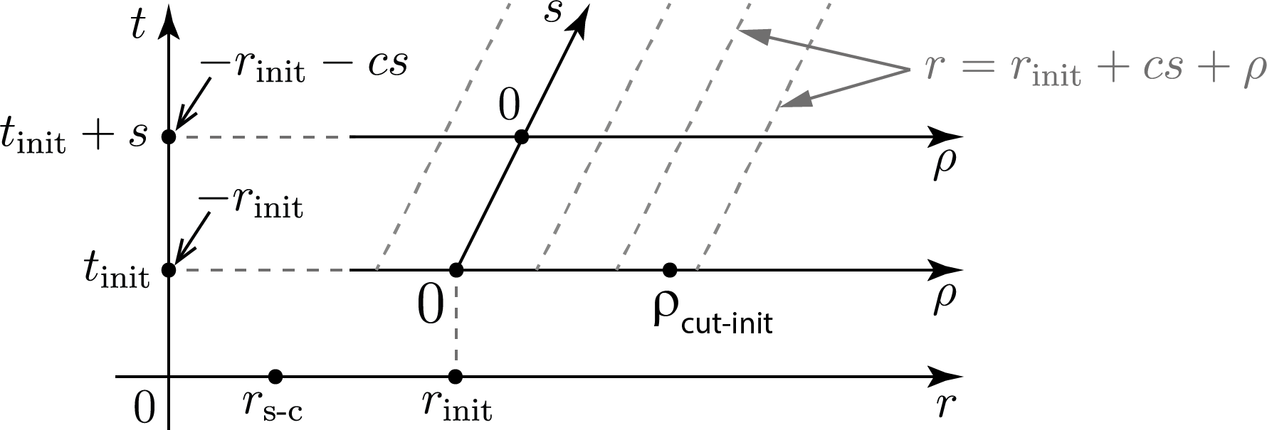
Figure 4.8: Space coordinate $\rho$ and time coordinate $s$ in the travelling frame, and parameters $t_{\textup{\text{init}}}$ and $r_{\textup{\text{init}}}$ and $c$ and $\rho_{\textup{\text{cut-init}}}$.

• the “initial time” $t_{\textup{\text{init}}}$ of the time interval of the relaxation;

• the position $r_{\textup{\text{init}}}$ of the origin of the travelling frame at initial time $t=t_{\textup{\text{init}}}$ (in practice it will be chosen equal to $r_{\textup{\text{esc}}}(t_{\textup{\text{init}}})$);

• the speed $c$ of the travelling frame;

• a quantity $\rho_{\textup{\text{cut-init}}}$ that will be the the position of the maximum point of the weight function $\rho\mapsto\chi(\rho,t_{\textup{\text{init}}})$ localizing energy at initial time $t=t_{\textup{\text{init}}}$ (this weight function is defined below); the subscript “cut” refers to the fact that this weight function displays a kind of “cut-off” on the interval between this maximum point and $+\infty$. Thus the maximum point is in some sense the point “where the cut-off begins”.

Let us make on these parameters the following hypotheses:

(4.35) $$0\leq t_{\textup{\text{init}}}\quad\text{and}\quad 0<c\leq c_{\textup{\text{no-esc}}}\quad\text{and}\quad 0\leq\rho_{\textup{\text{cut-init}}}\quad\text{and}\quad r_{\textup{\text{init}}}\geq r_{\textup{\text{s-c}}}\,.$$

For all $\rho$ in $[-r_{\textup{\text{init}}}-cs,+\infty)$ and $s$ in $[0,+\infty)$, let

$$v(\rho,s)=u^{\dagger}(r,t)\quad\text{where}\quad r=r_{\textup{\text{init}}}+cs+\rho\quad\text{and}\quad t=t_{\textup{\text{init}}}+s\,.$$

This function satisfies the differential system

(4.36) $$v_{s}-cv_{\rho}=-\nabla V^{\dagger}(v)+\frac{d-1}{r_{\textup{\text{init}}}+cs+\rho}v_{\rho}+v_{\rho\rho}\,.$$

Let $\kappa$ (rate of decrease of the weight functions), $c_{\textup{\text{cut}}}$ (speed of the cutoff point in the travelling frame), and $w_{\textup{\text{en}}}$ (coefficient of energy in the “firewall” function) be three positive quantities, small enough so that

(4.37) $$w_{\textup{\text{en}}}\Bigl{(}\frac{c_{\textup{\text{cut}}}(c+\kappa)}{2}+\frac{(c+\kappa+\frac{1}{2})^{2}}{4}\Bigr{)} \leq\frac{1}{4}\quad\text{and}\quad w_{\textup{\text{en}}}c_{\textup{\text{cut}}}(c+\kappa)\leq\frac{1}{4}$$

$$\text{and}\quad\frac{(c_{\textup{\text{cut}}}+\kappa)(c+\kappa)}{2} \leq\frac{\lambda_{\min}(m)}{16}$$

(these conditions will be used to prove inequality 4.55), and so that

(4.38) $$w_{\textup{\text{en}}}\leq w_{\textup{\text{en}},0}\,.$$

These quantities may be chosen as follows (first choose $\kappa$ and $c_{\textup{\text{cut}}}$ so that the third inequality of 4.37 be fulfilled, and then choose $w_{\textup{\text{en}}}$ according to the first two inequalities of 4.37 and to 4.38):

$$\kappa =\min\Bigl{(}\sqrt{\frac{\lambda_{\min}(m)}{32}},\frac{\lambda_{\min}(m)}{32c_{\textup{\text{no-esc}}}}\Bigr{)}\quad\text{and}\quad c_{\textup{\text{cut}}}=\frac{\lambda_{\min}(m)}{16(c_{\textup{\text{no-esc}}}+\kappa)}\,,$$

$$\text{and}\quad w_{\textup{\text{en}}} =\min\Bigl{(}\frac{1}{2c_{\textup{\text{cut}}}(c_{\textup{\text{no-esc}}}+\kappa)+(c_{\textup{\text{no-esc}}}+\kappa+1/2)^{2}},\frac{1}{4c_{\textup{\text{cut}}}(c_{\textup{\text{no-esc}}}+\kappa)},w_{\textup{\text{en}},0}\Bigr{)}\,.$$

Conditions 4.37 and 4.38 are very similar to those stated in [54], although slightly more stringent due to the curvature terms.

4.7.2 Localized energy

For every nonnegative quantity $s$, let us introduce the intervals

$$I_{\textup{\text{left}}}(s) =\bigl{[}-r_{\textup{\text{init}}}-cs,-r_{\textup{\text{init}}}-cs+r_{\textup{\text{s-c}}}\bigr{]}\,,$$

$$\text{and}\qquad I_{\textup{\text{main}}}(s) =\bigl{[}-r_{\textup{\text{init}}}-cs+r_{\textup{\text{s-c}}},\rho_{\textup{\text{cut-init}}}+c_{\textup{\text{cut}}}s\bigr{]}\,,$$

$$\text{and}\qquad I_{\textup{\text{right}}}(s) =[\rho_{\textup{\text{cut-init}}}+c_{\textup{\text{cut}}}s,+\infty)\,,$$

$$\text{and}\qquad I_{\textup{\text{tot}}}(s) =\bigl{[}-r_{\textup{\text{init}}}-cs,+\infty\bigr{)}=I_{\textup{\text{left}}}(s)\cup I_{\textup{\text{main}}}(s)\cup I_{\textup{\text{right}}}(s)\,,$$

see figure 4.9.

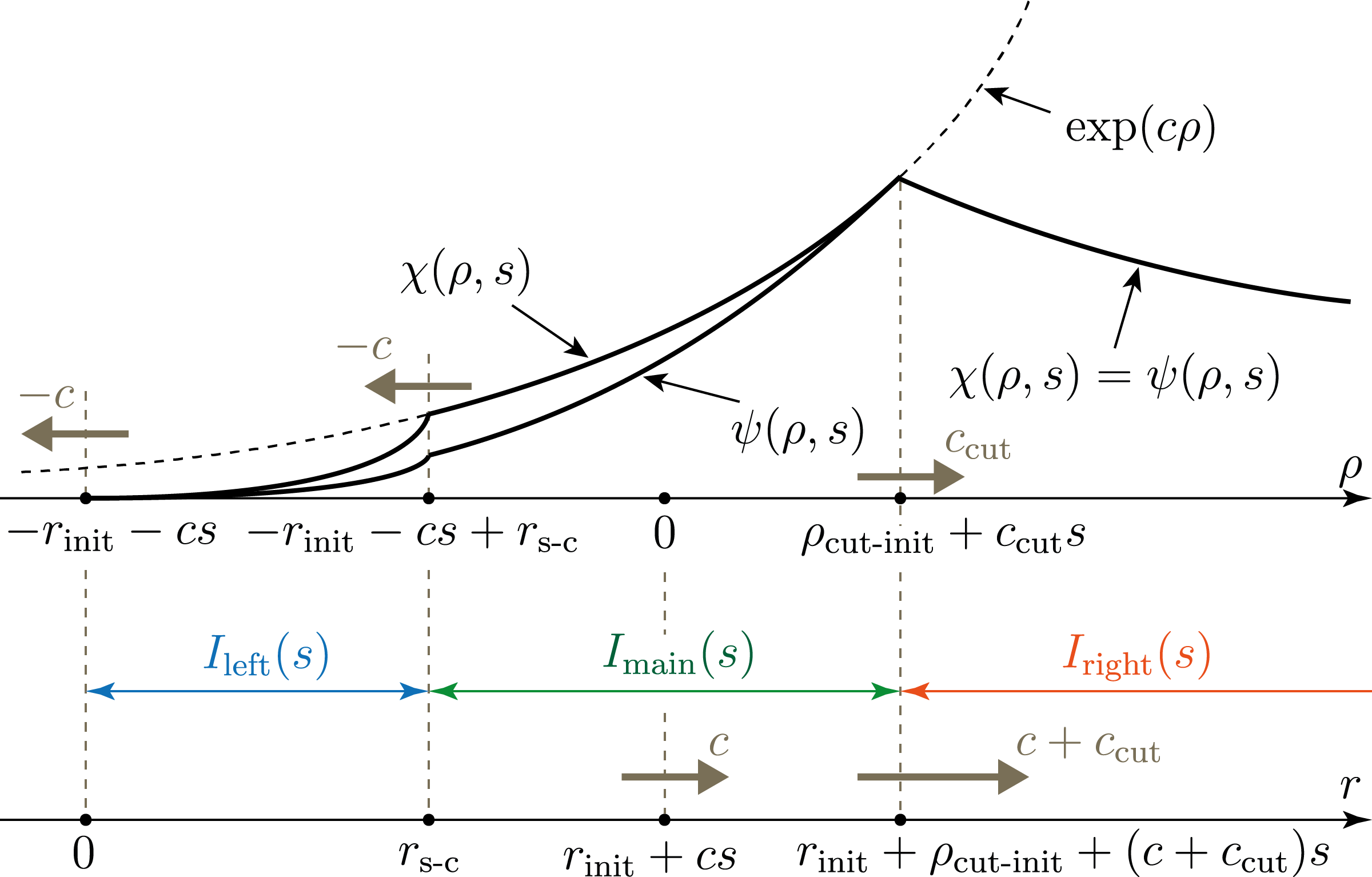
Figure 4.9: Intervals $I_{\textup{\text{left}}}(s)$ and $I_{\textup{\text{main}}}(s)$ and $I_{\textup{\text{right}}}(s)$ and graphs of the weight functions $\chi(y,s)$ and $\psi(y,s)$.

Observe that, since according to hypotheses 4.35 the quantity $r_{\textup{\text{init}}}$ is greater than or equal to $r_{\textup{\text{s-c}}}$, the interval $I_{\textup{\text{main}}}(s)$ is nonempty. Let us introduce the function $\chi(\rho,s)$ (weight function for the localized energy) defined as

$$\chi(\rho,s)=\left\{\begin{aligned} &\exp(c\rho)\Bigl{(}\frac{r_{\textup{\text{init}}}+cs+\rho}{r_{\textup{\text{s-c}}}}\Bigr{)}^{d-1}&&\text{if}\quad\rho\in I_{\textup{\text{left}}}(s)\,,\\ &\exp(c\rho)&&\text{if}\quad\rho\in I_{\textup{\text{main}}}(s)\,,\\ &\exp\Bigl{[}c(\rho_{\textup{\text{cut-init}}}+c_{\textup{\text{cut}}}s)-\kappa\bigl{(}\rho-(\rho_{\textup{\text{cut-init}}}+c_{\textup{\text{cut}}}s)\bigr{)}\Bigr{]}&&\text{if}\quad\rho\in I_{\textup{\text{right}}}(s)\,.\\ \end{aligned}\right.$$

For all $s$ in $[0,+\infty)$, let us define the “energy function” $\mathcal{E}(s)$ by

$$\mathcal{E}(s)=\int_{I_{\textup{\text{tot}}}(s)}\chi(\rho,s)\Bigl{(}\frac{1}{2}v_{\rho}(\rho,s)^{2}+V^{\dagger}\bigl{(}v(\rho,s)\bigr{)}\Bigr{)}\,d\rho\,.$$

4.7.3 Time derivative of the localized energy

For every nonnegative quantity $s$, let

$$\mathcal{D}(s)=\int_{I_{\textup{\text{tot}}}(s)}\chi(\rho,s)\,v_{s}(\rho,s)^{2}\,d\rho\,.$$

The aim of this sub-subsection is to prove the following lemma.

Lemma 4.6 (upper bound on time derivative of energy, first version).

There exist positive quantities $K_{\mathcal{E},\textup{\text{left}}}$ and $K_{\mathcal{E},\textup{\text{main}}}$, depending only on $V$ and $d$, such that, for every nonnegative quantity $s$, the following inequality holds:

(4.39) $$\mathcal{E}^{\prime}(s)\leq -\frac{1}{2}\mathcal{D}(s)+K_{\mathcal{E},\textup{\text{left}}}\exp\bigl{(}-cr_{\textup{\text{init}}}\bigr{)}$$

$$+K_{\mathcal{E},\textup{\text{main}}}\biggl{(}\exp\Bigl{(}-\frac{cr_{\textup{\text{init}}}}{2}\Bigr{)}+\frac{2}{r_{\textup{\text{init}}}}\exp\bigl{(}c(\rho_{\textup{\text{cut-init}}}+c_{\textup{\text{cut}}}s)\bigr{)}\biggr{)}$$

$$+\int_{I_{\textup{\text{right}}}(s)}\chi\biggl{(}c_{\textup{\text{cut}}}(c+\kappa)\Bigl{(}\frac{1}{2}v_{\rho}^{2}+V^{\dagger}(v)\Bigr{)}+\frac{(1/2+c+\kappa)^{2}}{2}v_{\rho}^{2}\biggr{)}\,d\rho\,.$$

Proof.

It follows from expression 3.6 for the derivative of a localized energy that

$$\mathcal{E}^{\prime}(s)= -\mathcal{D}(s)+\int_{I_{\textup{\text{tot}}}(s)}\chi_{s}\Bigl{(}\frac{1}{2}v_{\rho}^{2}+V^{\dagger}(v)\Bigr{)}\,d\rho$$

$$+\int_{I_{\textup{\text{tot}}}(s)}\Bigl{(}\frac{d-1}{r_{\textup{\text{init}}}+cs+\rho}\chi+c\chi-\chi_{\rho}\Bigr{)}v_{s}\cdot v_{\rho}\,d\rho\,.$$

It follows from the definition of $\chi$ that, for every real quantity $\rho$,

$$\chi_{s}(\rho,s)=\left\{\begin{aligned} &\frac{c(d-1)}{r_{\textup{\text{init}}}+cs+\rho}\chi(\rho,s)&&\text{if}\quad\rho\in I_{\textup{\text{left}}}(s)\,,\\ &0&&\text{if}\quad\rho\in I_{\textup{\text{main}}}(s)\,,\\ &c_{\textup{\text{cut}}}(c+\kappa)\chi(\rho,s)&&\text{if}\quad\rho\in I_{\textup{\text{right}}}(s)\,,\\ \end{aligned}\right.$$

and

$$\chi_{\rho}(\rho,s)=\left\{\begin{aligned} &c\chi(\rho,s)+\frac{d-1}{r_{\textup{\text{init}}}+cs+\rho}\chi(\rho,s)&&\text{if}\quad\rho\in I_{\textup{\text{left}}}(s)\,,\\ &c\chi(\rho,s)&&\text{if}\quad\rho\in I_{\textup{\text{main}}}(s)\,,\\ &-\kappa\chi(\rho,s)&&\text{if}\quad\rho\in I_{\textup{\text{right}}}(s)\,.\\ \end{aligned}\right.$$

thus

(4.40) $$\frac{d-1}{r_{\textup{\text{init}}}+cs+\rho}\chi(\rho,s)+c\chi(\rho,s) -\chi_{\rho}(\rho,s)=$$

$$\left\{\begin{aligned} &0&&\text{if}\quad\rho\in I_{\textup{\text{left}}}(s)\,,\\ &\frac{d-1}{r_{\textup{\text{init}}}+cs+\rho}\chi(\rho,s)&&\text{if}\quad\rho\in I_{\textup{\text{main}}}(s)\,,\\ &\Bigl{(}c+\kappa+\frac{d-1}{r_{\textup{\text{init}}}+cs+\rho}\Bigr{)}\chi(\rho,s)&&\text{if}\quad\rho\in I_{\textup{\text{right}}}(s)\,.\\ \end{aligned}\right.$$

As a consequence,

$$\mathcal{E}^{\prime}(s) =-\mathcal{D}(s)$$

$$+\int_{I_{\textup{\text{left}}}(s)}\chi\frac{c(d-1)}{r_{\textup{\text{init}}}+cs+\rho}\Bigl{(}\frac{1}{2}v_{\rho}^{2}+V^{\dagger}(v)\Bigr{)}\,d\rho$$

$$+\int_{I_{\textup{\text{main}}}(s)}\chi\frac{d-1}{r_{\textup{\text{init}}}+cs+\rho}v_{s}\cdot v_{\rho}\,d\rho$$

$$+\int_{I_{\textup{\text{right}}}(s)}\chi\biggl{(}c_{\textup{\text{cut}}}(c+\kappa)\Bigl{(}\frac{1}{2}v_{\rho}^{2}+V^{\dagger}(v)\Bigr{)}+\Bigl{(}\frac{d-1}{r_{\textup{\text{init}}}+cs+\rho}+c+\kappa\Bigr{)}v_{s}\cdot v_{\rho}\biggr{)}\,d\rho\,.$$

Polarizing the scalar products $v_{s}\cdot v_{\rho}$, it follows that

(4.41) $$\mathcal{E}^{\prime}(s)\leq -\frac{1}{2}\mathcal{D}(s)$$

$$+\int_{I_{\textup{\text{left}}}(s)}\chi\frac{c(d-1)}{r_{\textup{\text{init}}}+cs+\rho}\Bigl{(}\frac{1}{2}v_{\rho}^{2}+V^{\dagger}(v)\Bigr{)}\,d\rho$$

$$+\int_{I_{\textup{\text{main}}}(s)}\chi\frac{1}{2}\Bigl{(}\frac{d-1}{r_{\textup{\text{init}}}+cs+\rho}\Bigr{)}^{2}v_{\rho}^{2}\,d\rho$$

$$+\int_{I_{\textup{\text{right}}}(s)}\chi\biggl{(}c_{\textup{\text{cut}}}(c+\kappa)\Bigl{(}\frac{1}{2}v_{\rho}^{2}+V^{\dagger}(v)\Bigr{)}+\frac{1}{2}\Bigl{(}\frac{d-1}{r_{\textup{\text{init}}}+cs+\rho}+c+\kappa\Bigr{)}^{2}v_{\rho}^{2}\biggr{)}\,d\rho\,.$$

Let us make a brief comment on this inequality, in comparison with the (simpler) case $d=1$ (see [54, sub-subsection 4.7.5]).

Observe that the last term of this inequality (the integral over $I_{\textup{\text{right}}}(s)$) is very similar to the $d=1$ case. As in the $d=1$ case, its control will require the definition of a “firewall function” that will be defined in the next sub-subsection 4.7.4. Thus the main novelty with respect to the $d=1$ case is the existence of the two other integrals over $I_{\textup{\text{left}}}(s)$ and $I_{\textup{\text{main}}}(s)$ (according to the calculations above, the integral over $I_{\textup{\text{left}}}(s)$ follows from the fact that $\chi_{s}(\rho,s)$ is positive when $\rho$ belongs to this interval, and the integral over $I_{\textup{\text{main}}}(s)$ comes from the curvature term in system 4.36).

Unfortunately, the firewall function that will be defined in the next sub-subsection will be of no help to control these two terms, since the weight function $\psi(\rho,s)$ involved in its definition will have to be chosen much smaller than $\chi(\rho,s)$ on both intervals $I_{\textup{\text{left}}}(s)$ and $I_{\textup{\text{main}}}(s)$. As a consequence, these two terms need to be treated separately. The aim of the following two lemmas is to do this job, that is to provide appropriate upper bounds for these two terms (proof Lemma 4.6 will follow afterwards). The sole required feature of these bounds is that they should be small if the positive quantity $r_{\textup{\text{init}}}$ is large. ∎

Lemma 4.7 (upper bound for curvature term on $I_{\textup{\text{left}}}(s)$).

There exists a positive quantity $K_{\mathcal{E},\textup{\text{left}}}$, depending only on $V$ and $d$, such that, for every nonnegative quantity $s$, the following estimate holds:

(4.42) $$\int_{I_{\textup{\text{left}}}(s)}\chi\frac{c(d-1)}{r_{\textup{\text{init}}}+cs+\rho}\Bigl{(}\frac{1}{2}v_{\rho}^{2}+V^{\dagger}(v)\Bigr{)}\,d\rho\leq K_{\mathcal{E},\textup{\text{left}}}\exp\bigl{(}-cr_{\textup{\text{init}}}\bigr{)}\,.$$

Proof of Lemma 4.7.

For every nonnegative quantity $s$ and every $\rho$ in $I_{\textup{\text{left}}}(s)$,

$$\chi(\rho,s)\frac{c(d-1)}{r_{\textup{\text{init}}}+cs+\rho} =\frac{c(d-1)\exp(c\rho)}{r_{\textup{\text{s-c}}}}\Bigl{(}\frac{r_{\textup{\text{init}}}+cs+\rho}{r_{\textup{\text{s-c}}}}\Bigr{)}^{d-2}$$

$$\leq\frac{c(d-1)\exp(c\rho)}{r_{\textup{\text{s-c}}}}$$

(this inequality still holds if $d=1$, however recall that for clarity the $d$ equals $1$ case was excluded, thus $d$ is assumed to be not smaller than $2$). Thus,

$$\int_{I_{\textup{\text{left}}}(s)}\chi\frac{c(d-1)}{r_{\textup{\text{init}}}+cs+\rho}\,d\rho \leq\frac{d-1}{r_{\textup{\text{s-c}}}}\exp\bigl{(}c(-r_{\textup{\text{init}}}-cs+r_{\textup{\text{s-c}}}\bigr{)}$$

$$\leq\Bigl{(}\frac{d-1}{r_{\textup{\text{s-c}}}}\exp(cr_{\textup{\text{s-c}}})\Bigr{)}\exp(-cr_{\textup{\text{init}}})\,,$$

thus inequality 4.42 follows from the bound 4.35 on the speed $c$ and the bounds 4.1 for the solution. Lemma 4.7 is proved. ∎

Let us make the following additional hypothesis on the parameter $r_{\textup{\text{init}}}$:

(4.43) $$r_{\textup{\text{init}}}\geq 2r_{\textup{\text{s-c}}}\,.$$

Lemma 4.8 (upper bound for curvature term on $I_{\textup{\text{main}}}(s)$).

There exists a positive quantity $K_{\mathcal{E},\textup{\text{main}}}$, depending only on $V$ and $d$, such that, for every nonnegative quantity $s$, the following estimate holds:

(4.44) $$\int_{I_{\textup{\text{main}}}(s)}\chi\frac{1}{2}\Bigl{(}\frac{d-1}{r_{\textup{\text{init}}}+cs+\rho}\Bigr{)}^{2} v_{\rho}^{2}\,d\rho\leq$$

$$K_{\mathcal{E},\textup{\text{main}}} \biggl{(}\exp\Bigl{(}-\frac{cr_{\textup{\text{init}}}}{2}\Bigr{)}+\frac{2}{r_{\textup{\text{init}}}}\exp\bigl{(}c(\rho_{\textup{\text{cut-init}}}+c_{\textup{\text{cut}}}s)\bigr{)}\biggr{)}\,.$$

Proof of Lemma 4.8.

Let us introduce the integral:

$$J =\int_{I_{\textup{\text{main}}}(s)}\frac{\chi}{(r_{\textup{\text{init}}}+cs+\rho)^{2}}\,d\rho$$

$$=\int_{-r_{\textup{\text{init}}}-cs+r_{\textup{\text{s-c}}}}^{\rho_{\textup{\text{cut-init}}}+c_{\textup{\text{cut}}}s}\frac{\exp(c\,\rho)}{(r_{\textup{\text{init}}}+cs+\rho)^{2}}\,d\rho$$

$$=\exp\bigl{(}-cr_{\textup{\text{init}}}-c^{2}s\bigr{)}\int_{r_{\textup{\text{s-c}}}}^{r_{\textup{\text{init}}}+\rho_{\textup{\text{cut-init}}}+(c+c_{\textup{\text{cut}}})s}\frac{\exp(c\,r)}{r^{2}}\,dr\,.$$

To bound from above this expression, the integral may be cut into two pieces, namely:

$$J=\exp\bigl{(}-cr_{\textup{\text{init}}}-c^{2}s\bigr{)}\biggl{(}\int_{r_{\textup{\text{s-c}}}}^{r_{\textup{\text{init}}}/2}\frac{\exp(c\,r)}{r^{2}}\,dr+\int_{r_{\textup{\text{init}}}/2}^{r_{\textup{\text{init}}}+\rho_{\textup{\text{cut-init}}}+(c+c_{\textup{\text{cut}}})s}\frac{\exp(c\,r)}{r^{2}}\,dr\biggr{)}\,;$$

observe that according to hypothesis 4.43 the quantity $r_{\textup{\text{init}}}/2$ is not smaller than $r_{\textup{\text{s-c}}}$. Thus, bounding from above the two quantities $\exp(cr)$ in this expression (by replacing the quantity $r$ by the upper bound of the respective integration domain), it follows that

$$J\leq\frac{\exp\Bigl{(}-cr_{\textup{\text{init}}}/2-c^{2}s\Bigr{)}}{r_{\textup{\text{s-c}}}}+\frac{2}{r_{\textup{\text{init}}}}\exp\bigl{(}c(\rho_{\textup{\text{cut-init}}}+c_{\textup{\text{cut}}}s)\bigr{)}\,,$$

and since according to its definition 4.10 the quantity $r_{\textup{\text{s-c}}}$ is not smaller than $1$, it follows that

$$J\leq\exp\Bigl{(}-\frac{cr_{\textup{\text{init}}}}{2}\Bigr{)}+\frac{2}{r_{\textup{\text{init}}}}\exp\bigl{(}c(\rho_{\textup{\text{cut-init}}}+c_{\textup{\text{cut}}}s)\bigr{)}\,.$$

Thus inequality 4.44 follows from the bounds 4.1 for the solution. Lemma 4.8 is proved. ∎

End of the proof of Lemma 4.6.

Observe that, according to the definition 4.10 of $r_{\textup{\text{s-c}}}$, the quantity $(d-1)/(r_{\textup{\text{init}}}+cs+\rho)$ is not larger than $1/2$ as soon as $\rho$ is in $I_{\textup{\text{right}}}(s)$ (actually even in $I_{\textup{\text{main}}}(s)$). Thus inequality 4.39 of Lemma 4.6 follows from inequality 4.41 and from Lemmas 4.7 and 4.8. Lemma 4.6 is proved. ∎

4.7.4 Firewall function

A second function (the “firewall”) will now be defined, to get some control over the last term of the right-hand side of inequality 4.41. Let us introduce the function $\psi(y,s)$ (weight function for the firewall function) defined as follows (for every nonnegative quantity $s$ and every quantity $\rho$ in $I_{\textup{\text{tot}}}(s)$):

$$\psi(\rho,s)=\left\{\begin{aligned} &\exp\Bigl{[}\kappa\bigl{(}\rho-(\rho_{\textup{\text{cut-init}}}+c_{\textup{\text{cut}}}s)\bigr{)}\Bigr{]}\chi(\rho,s)&&\text{if}\quad\rho\in I_{\textup{\text{left}}}(s)\cup I_{\textup{\text{main}}}(s)\,,\\ &\chi(\rho,s)&&\text{if}\quad\rho\in I_{\textup{\text{right}}}(s)\,,\end{aligned}\right.$$

see figure 4.9; and, for every nonnegative quantity $s$, let us define the “firewall” function by

(4.45) $$\mathcal{F}(s)=\int_{I_{\textup{\text{tot}}}(s)}\psi(\rho,s)\biggl{(}w_{\textup{\text{en}}}\Bigl{(}\frac{1}{2}v_{\rho}(\rho,s)^{2}+V^{\dagger}\bigl{(}v(\rho,s)\bigr{)}\Bigr{)}+\frac{1}{2}v(\rho,s)^{2}\biggr{)}\,d\rho\,.$$

4.7.5 Energy decrease up to firewall

Lemma 4.9 (energy decrease up to firewall).

There exists a positive quantity $K_{\mathcal{E},\textup{\text{right}}}$, depending only on $V$, such that for every nonnegative quantity $s$,

(4.46) $$\mathcal{E}^{\prime}(s) \leq-\frac{1}{2}\mathcal{D}(s)+K_{\mathcal{E},\textup{\text{left}}}\exp\bigl{(}-cr_{\textup{\text{init}}}\bigr{)}$$

$$+K_{\mathcal{E},\textup{\text{main}}}\biggl{(}\exp\Bigl{(}-\frac{cr_{\textup{\text{init}}}}{2}\Bigr{)}+\frac{2}{r_{\textup{\text{init}}}}\exp\bigl{(}c(\rho_{\textup{\text{cut-init}}}+c_{\textup{\text{cut}}}s)\bigr{)}\biggr{)}+K_{\mathcal{E},\textup{\text{right}}}\mathcal{F}(s)\,.$$

Proof.

Let us introduce the following positive quantity (depending only on $V$):

$$K_{\mathcal{E},\textup{\text{right}}}=\frac{c_{\textup{\text{cut}}}(c_{\textup{\text{no-esc}}}+\kappa)+(1/2+c_{\textup{\text{no-esc}}}+\kappa)^{2}}{w_{\textup{\text{en}}}}\,.$$

Inequality 4.46 follows LABEL:{lem:ds_en_before_fire_last} (upper bound 4.39 on $\mathcal{E}^{\prime}(s)$). For a detailed justification, see [54, sub-subsection 4.7.6]. ∎

4.7.6 Relaxation scheme inequality, 1

Let $s_{\textup{\text{fin}}}$ be a nonnegative quantity (denoting the length of the time interval on which the relaxation scheme will be applied), and let us introduce the expression:

$$K_{\mathcal{E},\textup{\text{curv}}}(r,s,c)= K_{\mathcal{E},\textup{\text{left}}}\,s\exp\bigl{(}-cr\bigr{)}$$

$$+K_{\mathcal{E},\textup{\text{main}}}\,s\biggl{(}\exp\Bigl{(}-\frac{cr}{2}\Bigr{)}+\frac{2}{r_{\textup{\text{init}}}}\exp\bigl{(}c(\rho_{\textup{\text{cut-init}}}+c_{\textup{\text{cut}}}s)\bigr{)}\biggr{)}\,.$$

It follows from the previous inequality that

(4.47) $$\frac{1}{2}\int_{0}^{s_{\textup{\text{fin}}}}\mathcal{D}(s)\,ds\leq\ \mathcal{E}(0)-\mathcal{E}(s_{\textup{\text{fin}}})+K_{\mathcal{E},\textup{\text{curv}}}(r_{\textup{\text{init}}},s_{\textup{\text{fin}}},c)+K_{\mathcal{E},\textup{\text{right}}}\int_{0}^{s_{\textup{\text{fin}}}}\mathcal{F}(s)\,ds\,.$$

This “relaxation scheme inequality” is the core of the arguments carried out through this section 4 to prove Proposition 4.1. The crucial property of the “curvature term” $K_{\mathcal{E},\textup{\text{curv}}}(r,s,c)$ is that this quantity goes to $0$ as $r$ goes to $+\infty$, uniformly with respect to $s$ bounded and $c$ bounded away from $0$ and $+\infty$. The next goal is to gain some control over the firewall function (and as a consequence over the last term of this inequality).

4.7.7 Firewall linear decrease up to pollution

For every nonnegative quantity $s$, let us introduce the set (the domain of space where $v(\cdot,s)$ “Escapes” at distance $\delta_{\textup{\text{Esc}}}(m)$ from $0_{\mathbb{R}^{{d_{\textup{\text{st}}}}}}$) defined as

$$\Sigma_{\textup{\text{Esc}}}(s)=\{\rho\in I_{\textup{\text{main}}}(s)\cup I_{\textup{\text{right}}}(s):\left\lvert v(\rho,s)\right\rvert>\delta_{\textup{\text{Esc}}}(m)\}\,.$$

To make the connection with definition 4.18 of the related set $\Sigma_{\textup{\text{Esc}},0}(t)$, observe that, for every quantity $\rho$ in $I_{\textup{\text{tot}}}(s)$,

$$\rho\in\Sigma_{\textup{\text{Esc}}}(s)\iff r_{\textup{\text{init}}}+cs+\rho\in\Sigma_{\textup{\text{Esc}},0}(t_{\textup{\text{init}}}+s)\,.$$

The next step is the following lemma (observe the strong similarity with 4.3).

Lemma 4.10 (firewall linear decrease up to pollution).

There exist positive quantities $\nu_{\mathcal{F}}$ and $K_{\mathcal{F}}$ and $K_{\mathcal{F},\textup{\text{left}}}$ such that, for every nonnegative quantity $s$,

(4.48) $$\mathcal{F}^{\prime}(s)\leq-\nu_{\mathcal{F}}\mathcal{F}(s)+K_{\mathcal{F}}\int_{\Sigma_{\textup{\text{Esc}}}(s)}\psi(\rho,s)\,d\rho+K_{\mathcal{F},\textup{\text{left}}}\,\exp(-c\,r_{\textup{\text{init}}})\,.$$

The quantities $\nu_{\mathcal{F}}$ and $K_{\mathcal{F}}$ depend only on $V$ and $m$, whereas $K_{\mathcal{F},\textup{\text{left}}}$ depends additionally on $d$.

Proof.

According to expressions LABEL:ddt_loc_en_trav_fr,ddt_loc_L2_trav_fr for the time derivatives of a localized energy and a localized $L^{2}$ functional, for all $s$ in $[0,+\infty)$,

(4.49) $$\mathcal{F}^{\prime}(s)=\int_{I_{\textup{\text{tot}}}(s)}\Biggl{[} \psi\Bigl{(}-w_{\textup{\text{en}}}v_{s}^{2}-v\cdot\nabla V^{\dagger}(v)-v_{\rho}^{2}\Bigr{)}+\psi_{s}\biggl{(}w_{\textup{\text{en}}}\Bigl{(}\frac{1}{2}v_{\rho}^{2}+V^{\dagger}(v)\Bigr{)}+\frac{1}{2}v^{2}\biggr{)}$$

$$+\Bigl{(}\frac{d-1}{r_{\textup{\text{init}}}+cs+\rho}\psi+c\psi-\psi_{\rho}\Bigr{)}(w_{\textup{\text{en}}}v_{s}\cdot v_{\rho}+v\cdot v_{\rho})\Biggr{]}\,d\rho\,.$$

(this makes use of the “first” version of the time derivative of the $L^{2}$-functional written in 3.7, without the additional integration by parts of $c\psi-\psi_{\rho}$). The aim of the next calculations is to control the two last terms below this integral.

It follows from the definition of $\psi$ that, for every nonnegative quantity $s$,

(4.50) $$\psi_{s}(\rho,s)=\left\{\begin{aligned} &\Bigl{(}-\kappa c_{\textup{\text{cut}}}+\frac{c(d-1)}{r_{\textup{\text{init}}}+cs+\rho}\Bigr{)}\psi(\rho,s)&&\text{if}\quad\rho\in I_{\textup{\text{left}}}(s)\,,\\ &-\kappa c_{\textup{\text{cut}}}\psi(\rho,s)&&\text{if}\quad\rho\in I_{\textup{\text{main}}}(s)\,,\\ &c_{\textup{\text{cut}}}(c+\kappa)\psi(\rho,s)&&\text{if}\quad\rho\in I_{\textup{\text{right}}}(s)\,,\\ \end{aligned}\right.$$

and

$$\psi_{\rho}(\rho,s)=\left\{\begin{aligned} &\Bigl{(}\frac{d-1}{r_{\textup{\text{init}}}+cs+\rho}+c+\kappa\Bigr{)}\psi(\rho,s)&&\text{if}\quad\rho\in I_{\textup{\text{left}}}(s)\,,\\ &(c+\kappa)\psi(\rho,s)&&\text{if}\quad\rho\in I_{\textup{\text{main}}}(s)\,,\\ &-\kappa\psi(\rho,s)&&\text{if}\quad\rho\in I_{\textup{\text{right}}}(s)\,,\\ \end{aligned}\right.$$

thus

(4.51) $$\frac{d-1}{r_{\textup{\text{init}}}+cs+\rho}\psi(\rho,s)+ c\psi(\rho,s)-\psi_{\rho}(\rho,s)=$$

$$\left\{\begin{aligned} &-\kappa\psi(\rho,s)&&\text{if}\quad\rho\in I_{\textup{\text{left}}}(s)\,,\\ &\Bigl{(}\frac{d-1}{r_{\textup{\text{init}}}+cs+\rho}-\kappa\Bigr{)}\psi(\rho,s)&&\text{if}\quad\rho\in I_{\textup{\text{main}}}(s)\,,\\ &\Bigl{(}\frac{d-1}{r_{\textup{\text{init}}}+cs+\rho}+c+\kappa\Bigr{)}\psi(\rho,s)&&\text{if}\quad\rho\in I_{\textup{\text{right}}}(s)\,.\\ \end{aligned}\right.$$

As in the case $d=1$ (see [54]), the sole problematic term in the right-hand side of expression 4.49 (with respect to the conclusions of Lemma 4.10) is the product

$$(c\psi-\psi_{\rho})\,v\cdot v_{\rho}$$

on the interval $I_{\textup{\text{right}}}(s)$. As in [54], this term can be integrated by parts one more time to take advantage of the smallness of $\psi_{\rho\rho}-c\psi_{\rho}$ on $I_{\textup{\text{right}}}(s)$. There are several ways to proceed, since the integration by parts may be performed either only on $I_{\textup{\text{main}}}(s)\cup I_{\textup{\text{right}}}(s)$ or on the whole interval $I_{\textup{\text{tot}}}(s)$. Since the first option would create a border term at the left of $I_{\textup{\text{main}}}(s)$ let us go on with the second option. Doing so, it follows from 4.49 that

(4.52) $$\mathcal{F}^{\prime}(s)=\int_{I_{\textup{\text{tot}}}(s)}\Biggl{[} \psi\Bigl{(}-w_{\textup{\text{en}}}v_{s}^{2}-v\cdot\nabla V^{\dagger}(v)-v_{\rho}^{2}\Bigr{)}+\psi_{s}\biggl{(}w_{\textup{\text{en}}}\Bigl{(}\frac{1}{2}v_{\rho}^{2}+V^{\dagger}(v)\Bigr{)}+\frac{1}{2}v^{2}\biggr{)}$$

$$+w_{\textup{\text{en}}}\Bigl{(}\frac{d-1}{r_{\textup{\text{init}}}+cs+\rho}\psi+c\psi-\psi_{\rho}\Bigr{)}v_{s}\cdot v_{\rho}+\frac{d-1}{r_{\textup{\text{init}}}+cs+\rho}\psi v\cdot v_{\rho}$$

$$+\frac{\psi_{\rho\rho}-c\psi_{\rho}}{2}v^{2}\Biggr{]}\,d\rho\,.$$

It follows from the expression of $\psi_{\rho}$ above that, for every nonnegative quantity $s$,

(4.53) $$\psi_{\rho\rho}(\rho,s)-c\psi_{\rho}(\rho,s)\leq\theta(\rho,s)\quad\text{for all}\quad\rho\in I_{\textup{\text{tot}}}(s)\,,$$

where

$$\theta(\rho,s)=\left\{\begin{aligned} &\biggl{(}\kappa(c+\kappa)+\frac{(c+2\kappa)(d-1)}{r_{\textup{\text{init}}}+cs+\rho}+\frac{(d-1)(d-2)}{(r_{\textup{\text{init}}}+cs+\rho)^{2}}\biggr{)}\psi(\rho,s)&\quad\text{if}\quad\rho\in I_{\textup{\text{left}}}(s)\,,&\ \\ &\kappa(c+\kappa)\psi(\rho,s)&\quad\text{if}\quad\rho\not\in I_{\textup{\text{left}}}(s)\,.&\ \end{aligned}\right.$$

Indeed, $\psi_{\rho\rho}-c\psi_{\rho}$ equals $\theta$ plus two Dirac masses of negative weight (one at the junction between $I_{\textup{\text{left}}}(s)$ and $I_{\textup{\text{main}}}(s)$, and one at the junction between $I_{\textup{\text{main}}}(s)$ and $I_{\textup{\text{right}}}(s)$).

Observe that for every $\rho$ in the interval $I_{\textup{\text{main}}}(s)\cup I_{\textup{\text{right}}}(s)$, the quantity $r_{\textup{\text{init}}}+cs+\rho$ is not smaller than $r_{\textup{\text{s-c}}}$. As a consequence, it follows from equality 4.52 that, for every nonnegative quantity $s$,

(4.54) $$\mathcal{F}^{\prime}(s)\leq \int_{I_{\textup{\text{tot}}}(s)}\psi\Biggl{[}-w_{\textup{\text{en}}}v_{s}^{2}-v\cdot\nabla V^{\dagger}(v)-v_{\rho}^{2}+c_{\textup{\text{cut}}}(c+\kappa)\biggl{(}w_{\textup{\text{en}}}\Bigl{(}\frac{1}{2}v_{\rho}^{2}+V^{\dagger}(v)\Bigr{)}+\frac{1}{2}v^{2}\biggr{)}$$

$$+w_{\textup{\text{en}}}\Bigl{(}\frac{d-1}{r_{\textup{\text{s-c}}}}+c+\kappa\Bigr{)}\left\lvert v_{s}\cdot v_{\rho}\right\rvert+\frac{d-1}{r_{\textup{\text{s-c}}}}\left\lvert v\cdot v_{\rho}\right\rvert+\frac{\kappa(c+\kappa)}{2}v^{2}\Biggr{]}\,d\rho$$

$$+\mathcal{F}_{\textup{\text{res,\,left}}}(s)$$

where

$$\mathcal{F}_{\textup{\text{res,\,left}}}(s)= \int_{I_{\textup{\text{left}}}(s)}\frac{d-1}{r_{\textup{\text{init}}}+cs+\rho}\psi\Biggl{[}c\biggl{(}w_{\textup{\text{en}}}\Bigl{(}\frac{1}{2}v_{\rho}^{2}+V^{\dagger}(v)\Bigr{)}+\frac{1}{2}v^{2}\biggr{)}$$

$$+v\cdot v_{\rho}+\frac{1}{2}\biggl{(}(c+2\kappa)+\frac{(d-2)}{r_{\textup{\text{init}}}+cs+\rho}\biggr{)}v^{2}\Biggr{]}\,d\rho\,.$$

The following lemma deals with the “residual” term $\mathcal{F}_{\textup{\text{res,\,left}}}(s)$. ∎

Lemma 4.11 (control on the residual integral over $I_{\textup{\text{left}}}(s)$).

There exists a positive quantity $K_{\mathcal{F},\textup{\text{left}}}$, depending only on $V$ and $d$, such that, for every nonnegative quantity $s$, the following estimate holds:

$$\mathcal{F}_{\textup{\text{res,\,left}}}(s)\leq K_{\mathcal{F},\textup{\text{left}}}\,\exp(-cr_{\textup{\text{init}}})\,.$$

Proof of Lemma 4.11.

Since $\psi$ is smaller than $\chi$ on the interval $I_{\textup{\text{left}}}(s)$, the proof is identical to that of 4.7 (observe the vanishing term in $\mathcal{F}_{\textup{\text{res,\,left}}}(s)$ if $d=2$). ∎

End of the proof of Lemma 4.10.

Using the inequalities

$$\Bigl{(}\frac{d-1}{r_{\textup{\text{s-c}}}}+c+\kappa\Bigr{)}\left\lvert v_{s}\cdot v_{\rho}\right\rvert \leq v_{s}^{2}~+\frac{\Bigl{(}\frac{d-1}{r_{\textup{\text{s-c}}}}+c+\kappa\Bigr{)}^{2}}{4}v_{\rho}^{2}$$

$$\quad\text{and}\quad\left\lvert v\cdot v_{\rho}\right\rvert \leq\frac{1}{2}v^{2}~+\frac{1}{2}v_{\rho}^{2}\,,$$

it follows from inequality 4.54 and from Lemma 4.11 that, for every nonnegative quantity $s$,

$$\mathcal{F}^{\prime}(s)\leq \int_{I_{\textup{\text{tot}}}(s)}\psi\Biggl{[}\biggl{(}-1+w_{\textup{\text{en}}}\Bigl{(}\frac{c_{\textup{\text{cut}}}(c+\kappa)}{2}+\frac{(c+\kappa+\frac{d-1}{r_{\textup{\text{s-c}}}})^{2}}{4}\Bigr{)}+\frac{d-1}{2r_{\textup{\text{s-c}}}}\biggr{)}v_{\rho}^{2}$$

$$-v\cdot\nabla V^{\dagger}(v)+w_{\textup{\text{en}}}c_{\textup{\text{cut}}}(c+\kappa)\left\lvert V^{\dagger}(v)\right\rvert+\Bigl{(}\frac{d-1}{2r_{\textup{\text{s-c}}}}+\frac{(c_{\textup{\text{cut}}}+\kappa)(c+\kappa)}{2}\Bigr{)}v^{2}\Biggr{]}\,d\rho$$

$$+K_{\mathcal{F},\textup{\text{left}}}\,\exp(-cr_{\textup{\text{init}}})\,.$$

Since according to the definition 4.10 for $r_{\textup{\text{s-c}}}$ the quantity $(d-1)/r_{\textup{\text{s-c}}}$ is smaller than $1/2$ and than $\lambda_{\min}(m)/8$, it follows that

$$\mathcal{F}^{\prime}(s)\leq \int_{I_{\textup{\text{tot}}}(s)}\psi\Biggl{[}\biggl{(}-1+w_{\textup{\text{en}}}\Bigl{(}\frac{c_{\textup{\text{cut}}}(c+\kappa)}{2}+\frac{(c+\kappa+\frac{1}{2})^{2}}{4}\Bigr{)}+\frac{1}{4}\biggr{)}v_{\rho}^{2}$$

$$-v\cdot\nabla V^{\dagger}(v)+w_{\textup{\text{en}}}c_{\textup{\text{cut}}}(c+\kappa)\left\lvert V^{\dagger}(v)\right\rvert+\Bigl{(}\frac{\lambda_{\min}(m)}{16}+\frac{(c_{\textup{\text{cut}}}+\kappa)(c+\kappa)}{2}\Bigr{)}v^{2}\Biggr{]}\,d\rho$$

$$+K_{\mathcal{F},\textup{\text{left}}}\,\exp(-cr_{\textup{\text{init}}})\,,$$

and according to the properties 4.37 satisfied by the quantities $\kappa$ and $c_{\textup{\text{cut}}}$ and $w_{\textup{\text{en}}}$, it follows that

(4.55) $$\mathcal{F}^{\prime}(s)\leq \int_{I_{\textup{\text{tot}}}(s)}\psi\Bigl{(}-\frac{1}{2}v_{\rho}^{2}-v\cdot\nabla V^{\dagger}(v)+\frac{1}{4}\left\lvert V^{\dagger}(v)\right\rvert+\frac{\lambda_{\min}(m)}{8}v^{2}\Bigr{)}\,d\rho$$

$$+K_{\mathcal{F},\textup{\text{left}}}\,\exp(-cr_{\textup{\text{init}}})\,.$$

Let $\nu_{\mathcal{F}}$ be a positive quantity to be chosen below. It follows from the previous inequality and from the definition 4.45 of $\mathcal{F}(s)$ that

(4.56) $$\mathcal{F}^{\prime}(s)+\nu_{\mathcal{F}}\mathcal{F}(s)-K_{\mathcal{F},\textup{\text{left}}} \exp(-cr_{\textup{\text{init}}})\leq\int_{I_{\textup{\text{tot}}}(s)}\psi\biggl{[}-\frac{1}{2}(1-\nu_{\mathcal{F}}\,w_{\textup{\text{en}}})v_{\rho}^{2}-v\cdot\nabla V^{\dagger}(v)$$

$$+\Bigl{(}\frac{1}{4}+\nu_{\mathcal{F}}w_{\textup{\text{en}}}\Bigr{)}\left\lvert V^{\dagger}(v)\right\rvert+\Bigl{(}\frac{\lambda_{\min}(m)}{8}+\frac{\nu_{\mathcal{F}}}{2}\Bigr{)}v^{2}\biggr{]}\,d\rho\,.$$

In view of this inequality and of inequalities LABEL:v_nablaV_controls_square_around_loc_min_dag,v_nablaV_controls_pot_around_loc_min_dag, let us assume that $\nu_{\mathcal{F}}$ is small enough so that

(4.57) $$\nu_{\mathcal{F}}\,w_{\textup{\text{en}}}\leq 1\quad\text{and}\quad\nu_{\mathcal{F}}\,w_{\textup{\text{en}}}\leq\frac{1}{4}\quad\text{and}\quad\frac{\nu_{\mathcal{F}}}{2}\leq\frac{\lambda_{\min}(m)}{8}\,;$$

the quantity $\nu_{\mathcal{F}}$ may be chosen as

$$\nu_{\mathcal{F}}=\min\Bigl{(}\frac{1}{4w_{\textup{\text{en}}}},\frac{\lambda_{\min}(m)}{4}\Bigr{)}\,.$$

Then, it follows from 4.56 and 4.57 that

(4.58) $$\mathcal{F}^{\prime}(s)+\nu_{\mathcal{F}}\mathcal{F}(s)-K_{\mathcal{F},\textup{\text{left}}}\,\exp(-cr_{\textup{\text{init}}})\leq\int_{I_{\textup{\text{tot}}}(s)}\psi\Bigl{[}-v\cdot\nabla V^{\dagger}(v)+\frac{1}{2}\left\lvert V^{\dagger}(v)\right\rvert+\frac{\lambda_{\min}(m)}{4}v^{2}\Bigr{]}\,d\rho\,.$$

According to 4.6 and 4.7, the integrand of the integral at the right-hand side of this inequality is nonpositive as long as $\rho$ is not in $\Sigma_{\textup{\text{Esc}}}(s)$. Therefore this inequality still holds if the domain of integration of this integral is changed from $I_{\textup{\text{tot}}}(s)$ to $\Sigma_{\textup{\text{Esc}}}(s)$. Thus, introducing the quantity

$$K_{\mathcal{F}}=\max_{u\in\mathbb{R}^{{d_{\textup{\text{st}}}}},\ \left\lvert u\right\rvert\leq R_{\textup{\text{att}},\infty}}\Bigl{[}-(u-m)\cdot\nabla V(u)+\frac{1}{2}\left\lvert V(u)-V(m)\right\rvert+\frac{\lambda_{\min}(m)}{4}(u-m)^{2}\Bigr{]}$$

(which is positive and depends only on $V$ and $m$), inequality 4.48 follows from inequality 4.58. Lemma 4.10 is proved. ∎

4.7.8 Nonnegativity of the firewall

For all $s$ in $[0,+\infty)$,

(4.59) $$\mathcal{F}(s)\geq 0\,.$$

Indeed, in view of the property 3.13 concerning $w_{\textup{\text{en}},0}$ and since $w_{\textup{\text{en}}}$ is not larger than $w_{\textup{\text{en}},0}$, for all $s$ in $[0,+\infty)$ the following stronger coercivity property holds:

$$\mathcal{F}(s)\geq\min\Bigl{(}\frac{w_{\textup{\text{en}}}}{2},\frac{1}{4}\Bigr{)}\int_{I_{\textup{\text{tot}}}(s)}\psi(\rho,s)\bigl{(}v_{\rho}(\rho,s)^{2}+v(\rho,s)^{2}\bigr{)}\,d\rho\,.$$

4.7.9 Relaxation scheme inequality, 2

For every nonnegative quantity $s$, let

$$\mathcal{G}(s)=\int_{\Sigma_{\textup{\text{Esc}}}(s)}\psi(\rho,s)\,d\rho\,.$$

Integrating inequality 4.48 between $0$ and a nonnegative quantity $s_{\textup{\text{fin}}}$ yields, since according to 4.59 $\mathcal{F}(s_{\textup{\text{fin}}})$ is nonnegative,

$$\int_{0}^{s_{\textup{\text{fin}}}}\mathcal{F}(s)\,ds\leq\frac{1}{\nu_{\mathcal{F}}}\Bigl{(}\mathcal{F}(0)+K_{\mathcal{F}}\int_{0}^{s_{\textup{\text{fin}}}}\mathcal{G}(s)\,ds+K_{\mathcal{F},\textup{\text{left}}}\,s_{\textup{\text{fin}}}\,\exp(-c\,r_{\textup{\text{init}}})\Bigr{)}\,.$$

Thus, introducing the expression

$$\tilde{K}_{\mathcal{E},\textup{\text{curv}}}(r,s,c)=K_{\mathcal{E},\textup{\text{curv}}}(r,s,c)+\frac{K_{\mathcal{E},\textup{\text{right}}}\,K_{\mathcal{F},\textup{\text{left}}}\,s_{\textup{\text{fin}}}}{\nu_{\mathcal{F}}}\exp(-c\,r_{\textup{\text{init}}})\,,$$

the “relaxation scheme” inequality 4.47 becomes

(4.60) $$\frac{1}{2}\int_{0}^{s_{\textup{\text{fin}}}}\mathcal{D}(s)\,ds\leq \mathcal{E}(0)-\mathcal{E}(s_{\textup{\text{fin}}})+\tilde{K}_{\mathcal{E},\textup{\text{curv}}}\bigl{(}r_{\textup{\text{init}}},s_{\textup{\text{fin}}},c\bigr{)}$$

$$+\frac{K_{\mathcal{E},\textup{\text{right}}}}{\nu_{\mathcal{F}}}\Bigl{(}\mathcal{F}(0)+K_{\mathcal{F}}\int_{0}^{s_{\textup{\text{fin}}}}\mathcal{G}(s)\,ds\Bigr{)}\,.$$

Observe that, as was the case for $K_{\mathcal{E},\textup{\text{curv}}}(r,s,c)$, the “curvature term” $\tilde{K}_{\mathcal{E},\textup{\text{curv}}}(r,s,c)$ (still) goes to $0$ as $r$ goes to $+\infty$, uniformly with respect to $s$ bounded and $c$ bounded away from $0$ and $+\infty$. The next step is to gain some control over the quantity $\mathcal{G}(s)$.

4.7.10 Control over pollution in the time derivative of the firewall function

For every nonnegative quantity $s$ let

$$\rho_{\textup{\text{hom}}}(s) =r_{\textup{\text{hom}}}(t_{\textup{\text{init}}}+s)-r_{\textup{\text{init}}}-cs\,,$$

$$\text{and}\quad\rho_{\textup{\text{esc}}}(s) =r_{\textup{\text{esc}}}(t_{\textup{\text{init}}}+s)-r_{\textup{\text{init}}}-cs\,.$$

According to properties 4.31 for the set $\Sigma_{\textup{\text{Esc}},0}(t)$,

$$\Sigma_{\textup{\text{Esc}}}(s)\subset(-\infty,\rho_{\textup{\text{esc}}}(s)]\cup[\rho_{\textup{\text{hom}}}(s),+\infty)\,.$$

Let us introduce the quantities

$$\mathcal{G}_{\textup{\text{back}}}(s)=\int_{-r_{\textup{\text{init}}}-cs}^{\rho_{\textup{\text{esc}}}(s)}\psi(\rho,s)\,d\rho\quad\text{and}\quad\mathcal{G}_{\textup{\text{front}}}(s)=\int_{\rho_{\textup{\text{hom}}}(s)}^{+\infty}\psi(\rho,s)\,d\rho\,;$$

observe that, by definition — see 4.30 — the quantity $\rho_{\textup{\text{esc}}}(s)$ is greater than or equal to $r_{\textup{\text{s-c}}}-r_{\textup{\text{init}}}-cs$, and is therefore greater than $-r_{\textup{\text{init}}}-cs$. Then,

$$\mathcal{G}(s)\leq\mathcal{G}_{\textup{\text{back}}}(s)+\mathcal{G}_{\textup{\text{front}}}(s)\,.$$

Let us make the following hypothesis (required for the next lemma to hold):

(4.61) $$(c+\kappa)(\macc@depth\char 1\relax\frozen@everymath{\macc@group}\macc@set@skewchar\macc@nested@a 111{c}_{\textup{\text{esc-sup}}}-c)\leq\frac{\kappa c_{\textup{\text{cut}}}}{4}$$

(this hypothesis is satisfied as soon as $c$ is close enough to $\macc@depth\char 1\relax\frozen@everymath{\macc@group}\macc@set@skewchar\macc@nested@a 111{c}_{\textup{\text{esc-sup}}}$).

Lemma 4.12 (upper bounds on pollution terms in the derivative of the firewall).

There exists
a positive quantity $K[u_{0}]$, depending only on $V$ and on the initial condition $u_{0}$ (but not on the parameters $t_{\textup{\text{init}}}$ and $r_{\textup{\text{init}}}$ and $c$ and $\rho_{\textup{\text{cut-init}}}$ of the relaxation scheme) such that, for every nonnegative quantity $s$,

(4.62) $$\mathcal{G}_{\textup{\text{back}}}(s) \leq K[u_{0}]\exp(-\kappa\,\rho_{\textup{\text{cut-init}}})\exp\Big{(}-\frac{\kappa\,c_{\textup{\text{cut}}}}{2}s\Bigl{)}$$

$$\mathcal{G}_{\textup{\text{front}}}(s) \leq\frac{1}{\kappa}\exp\bigl{(}(c_{\textup{\text{no-esc}}}+1)\,\rho_{\textup{\text{cut-init}}}\bigr{)}\exp\bigl{(}(c_{\textup{\text{no-esc}}}+\kappa)(c_{\textup{\text{cut}}}+\kappa)s\bigr{)}\exp\bigl{(}-\kappa\,\rho_{\textup{\text{hom}}}(0)\bigr{)}\,.$$

Proof.

The proof is identical to that of [54, Lemma 4.10]. ∎

4.7.11 Relaxation scheme inequality, final

Let us introduce the quantity

$$K_{\mathcal{G},\textup{\text{back}}}[u_{0}]=\frac{2\,K_{\mathcal{E},\textup{\text{right}}}\,K_{\mathcal{F}}\,K[u_{0}]}{\nu_{\mathcal{F}}\,\kappa c_{\textup{\text{cut}}}}\,,$$

and, for every nonnegative quantity $s$, the quantity

$$K_{\mathcal{G},\textup{\text{front}}}(s)=\frac{K_{\mathcal{E},\textup{\text{right}}}\,K_{\mathcal{F}}}{\nu_{\mathcal{F}}\,\kappa\,(c_{\textup{\text{no-esc}}}+1)(c_{\textup{\text{cut}}}+1)}\exp\bigl{(}(c_{\textup{\text{no-esc}}}+1)(c_{\textup{\text{cut}}}+1)s\bigr{)}\,.$$

Then, for every nonnegative quantity $s_{\textup{\text{fin}}}$, according to inequalities 4.62, the “relaxation scheme” inequality 4.60 can be rewritten as

(4.63) $$\frac{1}{2}\int_{0}^{s_{\textup{\text{fin}}}}\mathcal{D}(s)\,ds\leq \mathcal{E}(0)-\mathcal{E}(s_{\textup{\text{fin}}})+\frac{K_{\mathcal{E},\textup{\text{right}}}}{\nu_{\mathcal{F}}}\mathcal{F}(0)+K_{\mathcal{G},\textup{\text{back}}}[u_{0}]\exp(-\kappa\,\rho_{\textup{\text{cut-init}}})$$

$$+K_{\mathcal{G},\textup{\text{front}}}(s_{\textup{\text{fin}}})\exp\bigl{(}(c_{\textup{\text{no-esc}}}+1)\,\rho_{\textup{\text{cut-init}}}\bigr{)}\exp\bigl{(}-\kappa\,\rho_{\textup{\text{hom}}}(0)\bigr{)}$$

$$+K_{\mathcal{E},\textup{\text{curv}}}\bigl{(}r_{\textup{\text{init}}},s_{\textup{\text{fin}}},c\bigr{)}\,.$$

Recall that the “curvature term” $K_{\mathcal{E},\textup{\text{curv}}}(r,s,c)$ goes to $0$ as $r$ goes to $+\infty$, uniformly with respect to $s$ bounded and $c$ bounded away from $0$ and $+\infty$. Recall by the way that this last inequality requires the additional hypothesis 4.43 made on the quantity $r_{\textup{\text{init}}}$ (namely, $r_{\textup{\text{init}}}$ should not be smaller than $2r_{\textup{\text{s-c}}}$).

4.8 Convergence of the mean invasion speed

The aim of this subsection is to prove the following proposition.

Proposition 4.13 (mean invasion speed).

The following equalities hold:

$$c_{\textup{\text{esc-inf}}}=c_{\textup{\text{esc-sup}}}=\macc@depth\char 1\relax\frozen@everymath{\macc@group}\macc@set@skewchar\macc@nested@a 111{c}_{\textup{\text{esc-sup}}}\,.$$

Proof.

Let us proceed by contradiction and assume that

$$c_{\textup{\text{esc-inf}}}<\macc@depth\char 1\relax\frozen@everymath{\macc@group}\macc@set@skewchar\macc@nested@a 111{c}_{\textup{\text{esc-sup}}}\,.$$

Then, let us take and fix a positive quantity $c$ satisfying the following conditions:

(4.64) $$c_{\textup{\text{esc-inf}}}<c<\macc@depth\char 1\relax\frozen@everymath{\macc@group}\macc@set@skewchar\macc@nested@a 111{c}_{\textup{\text{esc-sup}}}\leq c+\frac{\kappa c_{\textup{\text{cut}}}}{4(c_{\textup{\text{no-esc}}}+\kappa)}\quad\text{and}\quad\Phi_{c}(m)=\emptyset\,.$$

The first condition is satisfied as soon as $c$ is smaller than and close enough to $\macc@depth\char 1\relax\frozen@everymath{\macc@group}\macc@set@skewchar\macc@nested@a 111{c}_{\textup{\text{esc-sup}}}$, thus existence of a quantity $c$ satisfying the two conditions follows from hypothesis ($\textup{\text{H}}_{\textup{\text{disc-}}c}$).

The contradiction will follow from the relaxation scheme set up in subsection 4.7. The main ingredient is: since the set $\Phi_{c}(m)$ is empty, some dissipation must occur permanently around the escape point in a referential travelling at the speed $c$. This is stated by the following lemma.

Lemma 4.14 (nonzero dissipation in the absence of travelling front).

There exist positive quantities $L$ and $\varepsilon_{\textup{\text{dissip}}}$ such that, for every $t$ in $[0,+\infty)$, if the quantity $r_{\textup{\text{esc}}}(t)$ is greater than or equal to $L$, then the following inequality holds:

$$\left\lVert\rho\mapsto u_{t}\bigl{(}r_{\textup{\text{esc}}}(t)+\rho,t\bigr{)}+cu_{r}\bigl{(}r_{\textup{\text{esc}}}(t)+\rho,t\bigr{)}\right\rVert_{L^{2}([-L,L],\mathbb{R}^{{d_{\textup{\text{st}}}}})}\geq\varepsilon_{\textup{\text{dissip}}}\,.$$

Proof of Lemma 4.14.

Let us proceed by contradiction and assume that the converse is true. Then, for every positive integer $n$, there exists $t_{n}$ in $[0,+\infty)$ such that the quantity $r_{\textup{\text{esc}}}(t_{n})$ is greater than or equal to $n$ and such that

(4.65) $$\left\lVert\rho\mapsto u_{t}\bigl{(}r_{\textup{\text{esc}}}(t_{n})+\rho,t_{n}\bigr{)}+cu_{r}\bigl{(}r_{\textup{\text{esc}}}(t_{n})+\rho,t_{n}\bigr{)}\right\rVert_{L^{2}([-p,p],\mathbb{R}^{{d_{\textup{\text{st}}}}})}\leq\frac{1}{n}\,.$$

By compactness (Lemma 3.2), up to replacing the sequence $(t_{n})_{n\in\mathbb{N}}$ by a subsequence, there exists an entire solution $\macc@depth\char 1\relax\frozen@everymath{\macc@group}\macc@set@skewchar\macc@nested@a 111{u}$ of system 2.4 in

$$\mathcal{C}^{0}\left(\mathbb{R},\mathcal{C}^{2}_{\textup{\text{b}}}\bigl{(}\mathbb{R},\mathbb{R}^{{d_{\textup{\text{st}}}}}\bigr{)}\right)\cap\mathcal{C}^{1}\left(\mathbb{R},\mathcal{C}^{0}_{\textup{\text{b}}}\bigl{(}\mathbb{R},\mathbb{R}^{{d_{\textup{\text{st}}}}}\bigr{)}\right)\,,$$

such that, with the notation of 3.2,

$$D^{2,1}u(r_{\textup{\text{esc}}}(t_{n})+\cdot,t_{n}+\cdot)\to D^{2,1}\macc@depth\char 1\relax\frozen@everymath{\macc@group}\macc@set@skewchar\macc@nested@a 111{u}\quad\text{as}\quad n\to+\infty\,,$$

uniformly on every compact subset of $\mathbb{R}^{2}$. According to inequality 4.65, the function $\rho\mapsto\macc@depth\char 1\relax\frozen@everymath{\macc@group}\macc@set@skewchar\macc@nested@a 111{u}_{t}(\rho,0)+c\macc@depth\char 1\relax\frozen@everymath{\macc@group}\macc@set@skewchar\macc@nested@a 111{u}_{r}(\rho,0)$ vanishes identically, so that the function $\rho\mapsto\macc@depth\char 1\relax\frozen@everymath{\macc@group}\macc@set@skewchar\macc@nested@a 111{u}(\rho,0)$ is a solution of system 2.5 governing the profiles of waves travelling at the speed $c$ for system 2.4. According to the properties of the escape point LABEL:rEsc_resc_rHom,rHom_minus_resc,

$$\sup_{\rho\in[0,+\infty)}\left\lvert\phi(\rho)-m\right\rvert\leq\delta_{\textup{\text{Esc}}}(m)\,,$$

thus it follows from [54, Lemma 7.1] that $\phi(\rho)$ goes to $m$ as $\rho$ goes to $+\infty$. On the other hand, according to the bound 4.1 on the solution, $\left\lvert\phi(\cdot)\right\rvert$ is bounded (by $R_{\textup{\text{att}},\infty}$), and since $\Phi_{c}(m)$ is empty, it follows from [54, Lemma 7.1] that $\phi(\cdot)$ is identically equal to $m$, a contradiction with the definition of $r_{\textup{\text{esc}}}(\cdot)$. ∎

The remaining of the proof of Proposition 4.13 is identical to that of [54, Proposition 4.11], therefore it will not be reproduced here. ∎

According to Proposition 4.13, the three quantities $c_{\textup{\text{esc-inf}}}$ and $c_{\textup{\text{esc-sup}}}$ and $\macc@depth\char 1\relax\frozen@everymath{\macc@group}\macc@set@skewchar\macc@nested@a 111{c}_{\textup{\text{esc-sup}}}$ are equal; let

$$c_{\textup{\text{esc}}}$$

denote their common value.

4.9 Further control on the escape point

Proposition 4.15 (mean invasion speed, further control).

The following equality holds:

$$\underline{c}_{\textup{\text{esc-inf}}}=c_{\textup{\text{esc}}}\,.$$

Proof.

The proof is identical to that of [54, Proposition 4.17]. ∎

4.10 Dissipation approaches zero at regularly spaced times

For every $t$ in $[1,+\infty)$, the following set

$$\left\{\varepsilon\text{ in }(0,+\infty):\int_{-1/\varepsilon}^{+1/\varepsilon}\Bigl{(}u_{t}\bigl{(}r_{\textup{\text{esc}}}(t)+\rho,t\bigr{)}+c_{\textup{\text{esc}}}u_{r}\bigl{(}r_{\textup{\text{esc}}}(t)+\rho,t\bigr{)}\Bigr{)}^{2}\,d\rho\leq\varepsilon\right\}$$

is (according to the bounds 4.1 for the solution) a nonempty interval (which by the way is unbounded from above). Let

$$\delta_{\textup{\text{dissip}}}(t)$$

denote the infimum of this interval. This quantity measures to what extent the solution is, at time $t$ and around the escape point $r_{\textup{\text{esc}}}(t)$, close to be stationary in a frame travelling at the speed $c_{\textup{\text{esc}}}$. The next goal is to prove that

$$\delta_{\textup{\text{dissip}}}(t)\to 0\quad\text{as}\quad t\to+\infty\,.$$

Proposition 4.16 below can be viewed as a first step towards this goal.

Proposition 4.16 (regular occurrence of small dissipation).

For every positive quantity $\varepsilon$, there exists a positive quantity $T(\varepsilon)$ such that, for every $t$ in $[0,+\infty)$,

$$\inf_{t^{\prime}\in[t,t+T(\varepsilon)]}\delta_{\textup{\text{dissip}}}(t^{\prime})\leq\varepsilon\,.$$

Proof.

The proof is identical to that of [54, Proposition 4.19]. ∎

4.11 Relaxation

Proposition 4.17 (relaxation).

The following assertion holds:

$$\delta_{\textup{\text{dissip}}}(t)\to 0\quad\text{as}\quad t\to+\infty\,.$$

Proof.

The proof is identical to that of [54, Proposition 4.21]. ∎

4.12 Convergence

The end of the proof of 4.1 (“invasion implies convergence”) is a straightforward consequence of Proposition 4.17, and is identical to the case of space dimension one treated in [54, subsection 4.12 and subsection 4.13]. As mentioned above, the definition of the quantity $\delta_{\textup{\text{dissip}}}(t)$ is slightly different from that of [54], however since this quantity goes to $0$ as time goes to $+\infty$, limits of the profiles of the solution around the escape point $r_{\textup{\text{esc}}}(t)$ must (still with this new definition of $\delta_{\textup{\text{dissip}}}(t)$) necessarily be solutions of system 2.5 satisfied by the profiles of travelling fronts. Thus all arguments remain the same, and details will not be reproduced here. Proposition 4.1 is proved.

5 No invasion implies relaxation

5.1 Definitions and hypotheses

As everywhere else, let us consider a function $V$ in $\mathcal{C}^{2}(\mathbb{R}^{{d_{\textup{\text{st}}}}},\mathbb{R})$ satisfying the coercivity hypothesis $\text{H}_{\text{coerc}}$. As in section 4, let us consider a point $m$ in $\mathcal{M}$ and a solution $(r,t)\mapsto u(r,t)$ of system 1.2, and let us make the following hypothesis (which is identical to the one made in subsection 4.1):

$\textup{\text{(H}}_{\textup{\text{hom}}}\textup{\text{)}}$

There exists a positive quantity $c_{\textup{\text{hom}}}$ and a $\mathcal{C}^{1}$-function

$$r_{\textup{\text{hom}}}:[0,+\infty)\to\mathbb{R}\,,\quad\text{satisfying}\quad r_{\textup{\text{hom}}}^{\prime}(t)\to c_{\textup{\text{hom}}}\quad\text{as}\quad t\to+\infty\,,$$

such that, for every positive quantity $L$,

$$\sup_{\rho\in[-L,L]}\left\lvert u\bigl{(}r_{\textup{\text{hom}}}(t)+\rho,t\bigr{)}-m\right\rvert\to 0\quad\text{as}\quad t\to+\infty\,.$$

Let us define the function $t\mapsto r_{\textup{\text{Esc}}}(t)$ and the quantity $c_{\textup{\text{Esc}}}$ exactly as in subsection 4.1. By contrast with subsection 4.1 and the hypothesis ($\textup{\text{H}}_{\textup{\text{inv}}}$) made there, let us introduce the following (converse) hypothesis.

$\textup{\text{(H}}_{\textup{\text{no-inv}}}\textup{\text{)}}$

The quantity $c_{\textup{\text{Esc}}}$ is nonpositive.

5.2 Statement and proof

Proposition 5.1 (no invasion implies relaxation).

Assume that $V$ satisfies the coercivity hypothesis $\text{H}_{\text{coerc}}$ and, keeping the definitions and notation above, let us assume that the solution under consideration satisfies hypotheses ($\textup{\text{H}}_{\textup{\text{hom}}}$) and ($\textup{\text{H}}_{\textup{\text{no-inv}}}$). Then the following conclusions hold.

1. There exists a nonnegative quantity $\mathcal{E}_{\textup{\text{res-asympt}}}[u]$ (“residual asymptotic energy”) such that, for every quantity $c$ in the interval $(0,c_{\textup{\text{hom}}})$,

   $$\int_{0}^{ct}r^{d-1}\left(\frac{1}{2}u_{r}(r,t)^{2}~+V\bigl{(}u(r,t)\bigr{)}-V(m)\right)\,dr\to\mathcal{E}_{\textup{\text{res-asympt}}}[u]\quad\text{as}\quad t\to+\infty\,.$$

2. The quantity

   $$\sup_{r\in[0,r_{\textup{\text{hom}}}(t)]}\left\lvert u_{t}(r,t)\right\rvert$$

   goes to $0$ as time goes to $+\infty$.

3. For every quantity $c$ in the interval $(0,c_{\textup{\text{hom}}})$, the function

   $$t\mapsto\int_{0}^{ct}r^{d-1}u_{t}(r,t)^{2}\,dr$$

   is integrable on a neighbourhood of $+\infty$.

Proof.

[56, Theorem 2] states the same conclusions as Proposition 5.1 but in a broader setting, that is for solutions of system 1.1 without the hypothesis of radial symmetry. The reader is therefore referred to the proof provided in this reference. ∎

6 Relaxation implies convergence

6.1 Statement

As everywhere else, let us consider a function $V$ in $\mathcal{C}^{2}(\mathbb{R}^{{d_{\textup{\text{st}}}}},\mathbb{R})$ satisfying the coercivity hypothesis $\text{H}_{\text{coerc}}$. As in the previous section, let us consider a point $m$ in $\mathcal{M}$ and a solution $(r,t)\mapsto u(r,t)$ of system 1.2, and let us assume again that the same hypotheses ($\textup{\text{H}}_{\textup{\text{hom}}}$) and ($\textup{\text{H}}_{\textup{\text{no-inv}}}$) hold. Thus the conclusions of Proposition 5.1 hold. Let us keep all the notation introduced in the previous section, and let us make the following additional (generic) assumption.

$\textup{\text{(H}}_{\textup{\text{disc-stat-}}m}\textup{\text{)}}$

The set

$$\bigl{\{}\phi(0):\phi\in\Phi_{0,\textup{\text{centre}}}(m)\bigr{\}}$$

is totally discontinuous in $\mathbb{R}^{{d_{\textup{\text{st}}}}}$. That is, its connected components are singletons. Equivalently, the set $\Phi_{0,\textup{\text{centre}}}(m)$ is totally disconnected for the topology of compact convergence (uniform convergence on compact subsets of $[0,+\infty)$).

Note that hypothesis ($\textup{\text{H}}_{\textup{\text{disc-stat}}}$) stated in sub-subsection 2.4.3 is identical except that it concerns all elements of $\mathcal{M}$ instead of the single point $m$ as in ($\textup{\text{H}}_{\textup{\text{disc-stat-}}m}$). The aim of this section is to prove the additional conclusion provided by the following proposition.

Proposition 6.1 (relaxation implies convergence).

The following conclusions hold.

1. There exists a stationary solution $\phi$ in $\Phi_{0,\textup{\text{centre}}}(m)$ such that

   (6.1) $$\sup_{r\in[0,r_{\textup{\text{hom}}}(t)]}\left\lvert u(r,t)-\phi(r)\right\rvert\to 0\quad\text{as}\quad t\to+\infty\,.$$

2. The residual asymptotic energy $\mathcal{E}_{\textup{\text{res-asympt}}}[u]$ of the solution is equal to the energy $\mathcal{E}[\phi]$ of this stationary solution.

6.2 Properties of the Escape radius

Recall that, for every nonnegative time $t$, the escape radius $r_{\textup{\text{Esc}}}(t)$ is, according to its definition (see subsection 4.1), either equal to $-\infty$ or nonnegative.

6.2.1 Transversality

Lemma 6.2 (transversality at Escape radius).

There exists a positive time $t_{\textup{\text{Esc-transv}}}$ and a positive quantity $\varepsilon_{\textup{\text{Esc-transv}}}$ such that, for every time $t$ greater than or equal to $t_{\textup{\text{Esc-transv}}}$, if $r_{\textup{\text{Esc}}}(t)$ is not equal to $-\infty$, then

(6.2) $$\Bigl{(}u\bigl{(}r_{\textup{\text{Esc}}}(t),t\bigr{)}-m\Bigr{)}\cdot u_{r}\bigl{(}r_{\textup{\text{Esc}}}(t),t\bigr{)}\leq-\varepsilon_{\textup{\text{Esc-transv}}}\,.$$

Proof.

Let us proceed by contradiction and assume that there exists a sequence $(t_{n})_{n\in\mathbb{N}}$ such that $t_{n}$ goes to $+\infty$ as $n$ goes to $+\infty$ and such that, for every positive integer $n$,

(6.3) $$-\infty<r_{\textup{\text{Esc}}}(t_{n})\quad\text{and}\quad\Bigl{(}u\bigl{(}r_{\textup{\text{Esc}}}(t_{n}),t_{n}\bigr{)}-m\Bigr{)}\cdot u_{r}\bigl{(}r_{\textup{\text{Esc}}}(t_{n}),t_{n}\bigr{)}\geq-\frac{1}{n}\,.$$

Up to extracting a subsequence from the sequence $(t_{n})_{n\in\mathbb{N}}$, it may be assumed that one among the following two assertions holds:

1. $r_{\textup{\text{Esc}}}(t_{n})$ goes to $+\infty$ as $t$ goes to $+\infty$;

2. there exists a nonnegative (finite) quantity $r_{\textup{\text{Esc-}}\infty}$ such that $r_{\textup{\text{Esc}}}(t_{n})$ goes to $r_{\textup{\text{Esc-}}\infty}$ as $t$ goes to $+\infty$.

If assertion 1 holds, then, according to Lemma 3.2 and to conclusion 1 of Proposition 5.1, up to extracting again a subsequence from the sequence $(t_{n})_{n\in\mathbb{N}}$, it may be assumed that the functions $\rho\mapsto u\bigl{(}r_{\textup{\text{Esc}}}(t_{n})+\rho,t_{n}\bigr{)}$ converge, uniformly on every compact subset of $\mathbb{R}$, towards a $\mathcal{C}^{2}$-function $\phi:\mathbb{R}\to\mathbb{R}^{{d_{\textup{\text{st}}}}}$ satisfying the system

(6.4) $$\phi^{\prime\prime}=\nabla V(\phi)\,;$$

If assertion 2 holds, then, according to Lemma 3.3 and to conclusion 1 of Proposition 5.1, up to extracting again a subsequence from the sequence $(t_{n})_{n\in\mathbb{N}}$, the functions $r\mapsto u(r,t_{n})$ converge, uniformly on every compact subset of the interval $[0,+\infty)$, towards a $\mathcal{C}^{2}$-function $\hat{\phi}$ such that the function

$$\phi:[-r_{\textup{\text{Esc-}}\infty},+\infty)\to\mathbb{R}^{{d_{\textup{\text{st}}}}}\,,\quad\rho\mapsto\hat{\phi}(r_{\textup{\text{Esc-}}\infty}+\rho)$$

satisfies the system

(6.5) $$\phi^{\prime\prime}+\frac{d-1}{\rho+r_{\textup{\text{Esc-}}\infty}}\phi^{\prime}=\nabla V(\phi)\quad\text{with the boundary condition}\quad\phi^{\prime}(-r_{\textup{\text{Esc-}}\infty})=0\,;$$

In both cases, it follows from assumptions ($\textup{\text{H}}_{\textup{\text{hom}}}$) and ($\textup{\text{H}}_{\textup{\text{no-inv}}}$) and from the definition of $r_{\textup{\text{Esc}}}(t)$ that

$$\sup_{\rho\in[0,+\infty)}\left\lvert\phi(\rho)\right\rvert\leq\delta_{\textup{\text{Esc}}}(m)\,,$$

and it follows from assumption 6.3 that

(6.6) $$\bigl{(}\phi(0)-m\bigr{)}\cdot\phi^{\prime}(0)\geq 0\,.$$

In both cases, 8.1 applies to the function $\phi$, and inequality 6.6 conflicts conclusion 2 of this lemma, a contradiction. Lemma 6.2 is proved. ∎

6.2.2 Finiteness/infiniteness of Escape radius

Corollary 6.3.

One of the following two (mutually exclusive) alternatives occurs:

1. for every time $t$ greater than or equal to $t_{\textup{\text{Esc-transv}}}$, the quantity $r_{\textup{\text{Esc}}}(t)$ equals $-\infty$,

2. (or) for every time $t$ greater than or equal to $t_{\textup{\text{Esc-transv}}}$, the quantity $r_{\textup{\text{Esc}}}(t)$ is positive.

In addition, if the second alternative occurs, then the function $t\mapsto r_{\textup{\text{Esc}}}(t)$ is of class $\mathcal{C}^{1}$ on the interval $[t_{\textup{\text{Esc-transv}}},+\infty)$ and

(6.7) $$r_{\textup{\text{Esc}}}^{\prime}(t)\to 0\quad\text{as}\quad t\to+\infty\,.$$

Proof.

Let us introduce the function

$$f:[0,+\infty)\times[0,+\infty)\to\mathbb{R}\,,\quad(r,t)\mapsto\frac{1}{2}\Bigl{(}\bigl{(}u(r,t)-m\bigr{)}^{2}~-\delta_{\textup{\text{Esc}}}(m)^{2}\Bigr{)}\,.$$

According to the smoothness properties of the solution recalled in subsection 3.1, this function $f$ is of class $\mathcal{C}^{1}$ on $[0,+\infty)\times(0,+\infty)$. For every $(r,t)$ in $[0,+\infty)\times[0,+\infty)$, if $r_{\textup{\text{Esc}}}(t)$ is not equal to $-\infty$ then it is nonnegative and $f\bigl{(}r_{\textup{\text{Esc}}}(t),t\bigr{)}$ vanishes. If in addition $t$ is greater than or equal to the (positive) quantity $t_{\textup{\text{Esc-transv}}}$ defined in Lemma 6.2, then, according to inequality 6.2,

(6.8) $$\partial_{r}f\bigl{(}r_{\textup{\text{Esc}}}(t),t\bigr{)}=\Bigl{(}u\bigl{(}r_{\textup{\text{Esc}}}(t),t\bigr{)}-m\Bigr{)}\cdot u_{r}\bigl{(}r_{\textup{\text{Esc}}}(t),t\bigr{)}\leq-\varepsilon_{\textup{\text{Esc-transv}}}<0\,.$$

In this case, since according to the border condition in system 1.2 the quantity $u_{r}(0,t)$ vanishes, the quantity $r_{\textup{\text{Esc}}}(t)$ is necessarily positive. Let us introduce the set

$$\mathcal{T}=\bigl{\{}t\in[t_{\textup{\text{Esc-transv}}},+\infty):r_{\textup{\text{Esc}}}(t)>-\infty\bigr{\}}\,.$$

It follows from inequality 6.8, from the fact that $r_{\textup{\text{Esc}}}(t)$ is positive if $t$ is in $\mathcal{T}$, and from the Implicit Function Theorem that $\mathcal{T}$ is open in $[t_{\textup{\text{Esc-transv}}},+\infty)$. And it follows from the definition of $r_{\textup{\text{Esc}}}(t)$ that this set is closed in $[t_{\textup{\text{Esc-transv}}},+\infty)$. As a consequence, the set $\mathcal{T}$ is either empty or equal to $[t_{\textup{\text{Esc-transv}}},+\infty)$, and this proves the alternative (the first assertion of the lemma).

If $\mathcal{T}$ equals $[t_{\textup{\text{Esc-transv}}},+\infty)$, then it again follows from the Implicit Function Theorem that $t\mapsto r_{\textup{\text{Esc}}}(t)$ is of class $\mathcal{C}^{1}$, and for every time $t$ in this interval,

$$r_{\textup{\text{Esc}}}^{\prime}(t)=-\frac{\partial_{t}f\bigl{(}r_{\textup{\text{Esc}}}(t),t\bigr{)}}{\partial_{r}f\bigl{(}r_{\textup{\text{Esc}}}(t),t\bigr{)}}=-\frac{\Bigl{(}u\bigl{(}r_{\textup{\text{Esc}}}(t),t\bigr{)}-m\Bigr{)}\cdot u_{t}\bigl{(}r_{\textup{\text{Esc}}}(t),t\bigr{)}}{\Bigl{(}u\bigl{(}r_{\textup{\text{Esc}}}(t),t\bigr{)}-m\Bigr{)}\cdot u_{r}\bigl{(}r_{\textup{\text{Esc}}}(t),t\bigr{)}}\,.$$

According to conclusion 2 of Proposition 5.1, the numerator of this expression goes to $0$ as time goes to $+\infty$, while according to inequality 6.8 the absolute value of the denominator remains not smaller than $\varepsilon_{\textup{\text{Esc-transv}}}$; it follows that $r_{\textup{\text{Esc}}}^{\prime}(t)$ goes to $0$ as time goes to $+\infty$. Corollary 6.3 is proved. ∎

6.2.3 Infiniteness alternative for the Escape radius

Lemma 6.4 (infiniteness alternative for the Escape radius).

Assume that the first alternative of Corollary 6.3 occurs (that is, $r_{\textup{\text{Esc}}}(t)$ equals $-\infty$ for every time $t$ greater than or equal to $t_{\textup{\text{Esc-transv}}}$). Then,

$$\sup_{r\in[0,r_{\textup{\text{hom}}}(t)]}\left\lvert u(r,t)-m\right\rvert\to 0\quad\text{as}\quad t\to+\infty\,.$$

Proof.

Let us proceed by contradiction and assume that the converse holds. Then there exists a positive quantity $\varepsilon$ and a sequence $(t_{n},r_{n})_{n\in\mathbb{N}}$ in $\mathbb{R}^{2}$ such that $t_{n}$ goes to $+\infty$ as $t$ goes to $+\infty$ and, for every nonnegative integer $n$,

$$t_{n}\geq t_{\textup{\text{Esc-transv}}}\quad\text{and}\quad r_{n}\in\bigl{[}0,r_{\textup{\text{hom}}}(t_{n})\bigr{]}\quad\text{and}\quad\left\lvert u(r_{n},t_{n})-m\right\rvert\geq\varepsilon\,.$$

Up to extracting a subsequence, it may be assumed that one among the following two assertions holds:

1. $r_{n}$ goes to $+\infty$ as $t$ goes to $+\infty$;

2. there exists a nonnegative quantity $r_{\infty}$ such that $r_{n}$ goes to $r_{\infty}$ as $n$ goes to $+\infty$.

If assertion 1 holds, then, according to Lemma 3.2 and to conclusion 1 of Proposition 5.1, up to extracting again a subsequence, it may be assumed that the functions $\rho\mapsto u(r_{n}+\rho,t_{n})$ converge, uniformly on every compact subset of $\mathbb{R}$, towards a $\mathcal{C}^{2}$-function $\phi:\mathbb{R}\to\mathbb{R}^{{d_{\textup{\text{st}}}}}$ satisfying system 6.4, and satisfying

$$\sup_{\rho\in\mathbb{R}}\left\lvert\phi(\rho)-m\right\rvert\leq\delta_{\textup{\text{Esc}}}(m)\quad\text{and}\quad\left\lvert\phi(0)-m\right\rvert\geq\varepsilon\,,\quad\text{thus}\quad\phi\not\equiv m\,,$$

a contradiction with conclusion 4 of Lemma 8.1.

If assertion 2 holds, then, according to Lemma 3.3 and to conclusion 1 of Proposition 5.1, up to extracting again a subsequence, it may be assumed that the functions $r\mapsto u(r,t_{n})$ converge, uniformly on every compact subset of the interval $[0,+\infty)$, towards a $\mathcal{C}^{2}$-function $\hat{\phi}$ such that the function

$$\phi:[-r_{\infty},+\infty)\to\mathbb{R}^{{d_{\textup{\text{st}}}}}\,,\quad\rho\mapsto\hat{\phi}(r_{\infty}+\rho)$$

satisfies system 6.5, and satisfies

$$\sup_{\rho\in[-r_{\infty},+\infty)}\left\lvert\phi(\rho)-m\right\rvert\leq\delta_{\textup{\text{Esc}}}(m)\quad\text{and}\quad\left\lvert\phi(0)-m\right\rvert\geq\varepsilon\,,\quad\text{thus}\quad\phi\not\equiv m\,,$$

again a contradiction with conclusion 4 of Lemma 8.1. ∎

6.2.4 Non divergence towards infinity in the finiteness alternative for the Escape radius

If the first alternative of Corollary 6.3 occurs, then it follows from Lemma 6.4 that the conclusion of Proposition 6.1 holds. The following proposition is the main step towards completing the proof of Proposition 6.1 when the second alternative of Corollary 6.3 occurs.

Proposition 6.5 (non divergence towards infinity for the Escape radius).

Assume that the second alternative of Corollary 6.3 occurs, that is $r_{\textup{\text{Esc}}}(t)$ is positive for all $t$ in $[t_{\textup{\text{Esc-transv}}},+\infty)$. Then the following inequality holds:

$$\liminf_{t\to+\infty}r_{\textup{\text{Esc}}}(t)<+\infty\,.$$

Proof.

Let us proceed by contradiction and assume that

(6.9) $$r_{\textup{\text{Esc}}}(t)\to+\infty\quad\text{as}\quad t\to+\infty\,.$$

Let $t$ be a time greater than or equal to $t_{\textup{\text{Esc-transv}}}$. Proceeding as in the proof of Pokhozhaev’s identity (see for instance [4]), the equality obtained by integrating over space the scalar product of system 1.2 by $r^{d}u_{r}$ (that is, by $ru_{r}$ times the factor $r^{d-1}$ induced by the Lebesgue measure on $\mathbb{R}^{d}$) will be considered. The domain of integration will be the interval $\bigl{[}0,2r_{\textup{\text{Esc}}}(t)\bigr{]}$. To simplify the writing, let us denote by $R$ the quantity $2r_{\textup{\text{Esc}}}(t)$. This leads to the following three integrals:

$$\mathcal{I}_{1}(t) =\int_{0}^{R}r^{d}u_{r}(r,t)\cdot u_{t}(r,t)\,,$$

$$\text{and}\quad\mathcal{I}_{2}(t) =-\int_{0}^{R}r^{d}u_{r}(r,t)\cdot\nabla V\bigl{(}u(r,t)\bigr{)}\,dr\,,$$

$$\text{and}\quad\mathcal{I}_{3}(t) =\int_{0}^{R}r^{d}u_{r}(r,t)\cdot\left(\frac{d-1}{r}u_{r}(r,t)+u_{rr}(r,t)\right)\,dr\,.$$

According to system 1.2,

(6.10) $$\mathcal{I}_{1}(t)=\mathcal{I}_{2}(t)+\mathcal{I}_{3}(t)\,.$$

Let us introduce the “normalized” potential $V^{\ddagger}$ defined as

$$V^{\ddagger}(v)=V(v)-V(m)\,,$$

and let us introduce the additional notation:

(6.11) $$\mathcal{K}(t) =\int_{0}^{R}r^{d-1}\frac{1}{2}u_{r}(r,t)^{2}\,dr\,,\quad \quad\mathcal{V}(t) =\int_{0}^{R}r^{d-1}V^{\ddagger}\bigl{(}u(r,t)\bigr{)}\,dr\,,$$ and

$$\text{and}\quad\tilde{\mathcal{E}}(t) =\mathcal{K}(t)+\mathcal{V}(t)\,,\quad \quad\tilde{\mathcal{D}}(t) =\int_{0}^{R}r^{d-1}u_{t}(r,t)^{2}\,dr\,,$$ and

and

$$H^{\ddagger}(t)=\frac{1}{2}u(R,t)^{2}-V^{\ddagger}\bigl{(}u(R,t)\bigr{)}\,.$$

Observe that $\mathcal{K}(t)$ and $\mathcal{V}(t)$ respectively denote the kinetic part and the potential part of the energy $\tilde{\mathcal{E}}(t)$ and $\tilde{\mathcal{D}}(t)$ denotes its dissipation, while the expression of $H^{\ddagger}(t)$ is the (normalized) Hamiltonian of the system governing stationary solutions of system 1.2 in the large radius limit (in the notation $\tilde{\mathcal{E}}(t)$ and $\tilde{\mathcal{D}}(t)$, the “tilde” is here only to avoid any confusion with the quantities $\mathcal{E}(t)$ and $\mathcal{D}(t)$ introduced in subsection 4.7). All this notation naturally leads to rephrase equality 6.10, as the following calculation shows:

$$\mathcal{I}_{2}(t) =-\int_{0}^{R}r^{d}\partial_{r}V^{\ddagger}\bigl{(}u(r,t)\bigr{)}\,dr$$

$$=-R^{d}V^{\ddagger}\bigl{(}u(R,t)\bigr{)}+\int_{0}^{R}\partial_{r}(r^{d})V^{\ddagger}\bigl{(}u(r,t)\bigr{)}\,dr$$

$$=-R^{d}V^{\ddagger}\bigl{(}u(R,t)\bigr{)}+d\times\mathcal{V}(t)\,,$$

and

$$\mathcal{I}_{3}(t) =\int_{0}^{R}\Bigl{(}(d-1)r^{d-1}u_{r}(r,t)^{2}+r^{d}u_{r}(r,t)\cdot u_{rr}(r,t)\Bigr{)}\,dr$$

$$=2(d-1)\mathcal{K}(t)+\int_{0}^{R}r^{d}\partial_{r}\left(\frac{u_{r}(r,t)^{2}}{2}\right)\,dr$$

$$=2(d-1)\mathcal{K}(t)+R^{d}\frac{u_{r}(R,t)^{2}}{2}-d\mathcal{K}(t)$$

$$=(d-2)\mathcal{K}(t)+R^{d}\frac{u_{r}(R,t)^{2}}{2}\,.$$

Thus it follows from equality 6.10 that

(6.12) $$d\times\tilde{\mathcal{E}}(t)-2~\mathcal{K}(t)+R^{d}H^{\ddagger}(t)=\int_{0}^{R}r^{d}u_{r}(r,t)\cdot u_{t}(r,t)\,dr\,.$$

Observe that the first two terms of the left-hand side of this equality correspond to Pokhozhaev’s identity 2.3. According to Cauchy–Schwarz inequality,

(6.13) $$\left\lvert\int_{0}^{R}r^{d}u_{r}(r,t)\cdot u_{t}(r,t)\,dr\right\rvert^{2} \leq 2\mathcal{K}(t)\int_{0}^{R}r^{d+1}u_{t}(r,t)^{2}\,dr$$

$$\leq 2\mathcal{K}(t)\,R^{2}\,\tilde{\mathcal{D}}(t)\,.$$

It follows from equality 6.12 and inequality 6.13 that

$$\tilde{\mathcal{D}}(t) \geq\frac{1}{2R^{2}\mathcal{K}(t)}\left\lvert 2~\mathcal{K}(t)-d\times\tilde{\mathcal{E}}(t)-R^{d}H^{\ddagger}(t)\right\rvert^{2}$$

$$=\frac{\mathcal{K}(t)}{R^{2}}\left\lvert 1~-\frac{d\times\tilde{\mathcal{E}}(t)}{2\mathcal{K}(t)}-\frac{R^{d}H^{\ddagger}(t)}{2\mathcal{K}(t)}\right\rvert^{2}\,,$$

provided that $\mathcal{K}(t)$ is positive, which is true at least for $t$ positive large enough according to Lemma 6.7 below. Substituting the notation $R$ with its value $2r_{\textup{\text{Esc}}}(t)$, this last inequality reads:

(6.14) $$\tilde{\mathcal{D}}(t)\geq\frac{\mathcal{K}(t)}{4r_{\textup{\text{Esc}}}(t)^{2}}\left\lvert 1~-\frac{d\times\tilde{\mathcal{E}}(t)}{2\mathcal{K}(t)}-\frac{\bigl{(}2r_{\textup{\text{Esc}}}(t)\bigr{)}^{d}H^{\ddagger}(t)}{2\mathcal{K}(t)}\right\rvert^{2}\,.$$

A contradiction will follow from this inequality and the following four lemmas. ∎

Lemma 6.6.

The function $t\mapsto\tilde{\mathcal{D}}(t)$ is integrable on the interval $[t_{\textup{\text{Esc-transv}}},+\infty)$.

Proof of Lemma 6.6.

This statement follows from conclusion 3 of Proposition 5.1. ∎

Lemma 6.7.

The following inequality hold:

(6.15) $$\liminf_{t\to+\infty}\frac{\mathcal{K}(t)}{r_{\textup{\text{Esc}}}(t)}>0\,.$$

Proof of Lemma 6.7.

It is sufficient to prove the following inequality, which is stronger than inequality 6.15 since $d$ is not smaller than $2$:

(6.16) $$\liminf_{t\to+\infty}\frac{\mathcal{K}(t)}{r_{\textup{\text{Esc}}}(t)^{d-1}}>0\,.$$

To prove this stronger inequality 6.16, let us proceed by contradiction and assume that there exists a sequence $(t_{n})_{n\in\mathbb{N}}$ of times greater than or equal to $t_{\textup{\text{Esc-transv}}}$ and going to $+\infty$ as $n$ goes to $+\infty$, such that

(6.17) $$\frac{\mathcal{K}(t_{n})}{r_{\textup{\text{Esc}}}(t_{n})^{d-1}}\to 0\quad\text{as}\quad t\to+\infty\,.$$

Observe that, for every large enough positive integer $n$, according to the assumption 6.9 and to the definition 6.11 of $\mathcal{K}(\cdot)$,

$$\frac{\mathcal{K}(t_{n})}{r_{\textup{\text{Esc}}}(t_{n})^{d-1}} \geq\frac{1}{r_{\textup{\text{Esc}}}(t_{n})^{d-1}}\int_{r_{\textup{\text{Esc}}}(t_{n})-1}^{r_{\textup{\text{Esc}}}(t_{n})+1}r^{d-1}\frac{1}{2}u_{r}(r,t_{n})^{2}\,dr$$

$$\geq\frac{\bigl{(}r_{\textup{\text{Esc}}}(t_{n})-1\bigr{)}^{d-1}}{2r_{\textup{\text{Esc}}}(t_{n})^{d-1}}\int_{r_{\textup{\text{Esc}}}(t_{n})-1}^{r_{\textup{\text{Esc}}}(t_{n})+1}u_{r}(r,t_{n})^{2}\,dr\,,$$

thus it follows from assumption 6.17 that

$$\int_{r_{\textup{\text{Esc}}}(t_{n})-1}^{r_{\textup{\text{Esc}}}(t_{n})+1}u_{r}(r,t_{n})^{2}\,dr\to 0\quad\text{as}\quad t\to+\infty\,,$$

and as a consequence, it follows from the bounds 3.1 on the solution that

$$u_{r}\bigl{(}r_{\textup{\text{Esc}}}(t_{n}),t_{n}\bigr{)}\to 0\quad\text{as}\quad t\to+\infty\,,$$

a contradiction with inequality 6.8. Lemma 6.7 is proved. ∎

Note that according to assumption 6.9, it follows from this inequality 6.15 that $\mathcal{K}(t)$ goes to $+\infty$ as $t$ goes to $+\infty$.

Lemma 6.8.

The following inequality holds:

(6.18) $$\limsup_{t\to+\infty}\tilde{\mathcal{E}}(t)<+\infty\,.$$

Proof of Lemma 6.8.

For every quantity $c$ in the interval $(0,c_{\textup{\text{hom}}})$, the quantity $2r_{\textup{\text{Esc}}}(t)$ is less than $ct$ as soon as $t$ is large enough positive, and in this case it follows from the definition of $r_{\textup{\text{Esc}}}(t)$ that the integrand

$$\frac{1}{2}u_{r}(r,t)^{2}+V\bigl{(}u(r,t)\bigr{)}-V(m)$$

of the energy is nonnegative for $r$ in the interval $\bigl{[}2r_{\textup{\text{Esc}}}(t),ct\bigr{]}$. Thus inequality 6.18 follows from conclusion 1 of Proposition 5.1. ∎

Lemma 6.9.

The following limit holds:

(6.19) $$r_{\textup{\text{Esc}}}(t)^{d}H^{\ddagger}(t)\to 0\quad\text{as}\quad t\to+\infty\,.$$

Proof of Lemma 6.9.

Let us call upon the notation $r_{\textup{\text{s-c}}}$ and $\psi_{0}(\cdot)$ and $\mathcal{F}_{0}(\cdot,\cdot)$ introduced in sub-subsection 4.4.1. Let $t_{1}$ denote a time greater than or equal to $t_{\textup{\text{Esc-transv}}}$ and large enough so that, for every time $t$ greater than or equal to $t_{1}$, the quantity $2r_{\textup{\text{Esc}}}(t)$ is greater than $r_{\textup{\text{s-c}}}$. For every time $t$ greater than or equal to $t_{1}$, let

$$\mathcal{F}_{1}(t)=\mathcal{F}_{0}\bigl{(}2r_{\textup{\text{Esc}}}(t),t\bigr{)}\,.$$

Then, for $t$ greater than or equal to $t_{1}$,

$$\mathcal{F}_{1}^{\prime}(t)=\partial_{t}\mathcal{F}_{0}\bigl{(}2r_{\textup{\text{Esc}}}(t),t\bigr{)}+2~r_{\textup{\text{Esc}}}^{\prime}(t)\partial_{\macc@depth\char 1\relax\frozen@everymath{\macc@group}\macc@set@skewchar\macc@nested@a 111{r}}\mathcal{F}_{0}\bigl{(}2r_{\textup{\text{Esc}}}(t),t\bigr{)}\,.$$

For every quantity $\macc@depth\char 1\relax\frozen@everymath{\macc@group}\macc@set@skewchar\macc@nested@a 111{r}$ greater than or equal to $r_{\textup{\text{s-c}}}$, according to the definitions of $\psi_{0}(\cdot)$ and $T_{\macc@depth\char 1\relax\frozen@everymath{\macc@group}\macc@set@skewchar\macc@nested@a 111{r}}\psi_{0}(\cdot)$,

$$\left\lvert\partial_{\macc@depth\char 1\relax\frozen@everymath{\macc@group}\macc@set@skewchar\macc@nested@a 111{r}}\bigl{(}T_{\macc@depth\char 1\relax\frozen@everymath{\macc@group}\macc@set@skewchar\macc@nested@a 111{r}}\psi_{0}\bigr{)}(r)\right\rvert=\kappa_{0}T_{\macc@depth\char 1\relax\frozen@everymath{\macc@group}\macc@set@skewchar\macc@nested@a 111{r}}\psi_{0}(r)$$

(except at the two points $r_{\textup{\text{s-c}}}$ and $\macc@depth\char 1\relax\frozen@everymath{\macc@group}\macc@set@skewchar\macc@nested@a 111{r}$ where this partial derivative is not defined). It follows that

$$\left\lvert\partial_{\macc@depth\char 1\relax\frozen@everymath{\macc@group}\macc@set@skewchar\macc@nested@a 111{r}}\mathcal{F}_{0}(\macc@depth\char 1\relax\frozen@everymath{\macc@group}\macc@set@skewchar\macc@nested@a 111{r},t)\right\rvert\leq\kappa_{0}\mathcal{F}_{0}(\macc@depth\char 1\relax\frozen@everymath{\macc@group}\macc@set@skewchar\macc@nested@a 111{r},t)\,.$$

As a consequence, it follows from inequality 4.19 of Lemma 4.3 that, for every time $t$ greater than or equal to $t_{1}$, with the notation of Lemma 4.3,

(6.20) $$\mathcal{F}_{1}^{\prime}(t)\leq\bigl{(}-\nu_{\mathcal{F}_{0}}+2\kappa_{0}r_{\textup{\text{Esc}}}^{\prime}(t)\bigr{)}\mathcal{F}_{1}(t)+K_{\mathcal{F}_{0}}\int_{\Sigma_{\textup{\text{Esc}},0}(t)}T_{2r_{\textup{\text{Esc}}}(t)}\psi_{0}(r)\,dr\,.$$

Up to replacing the time $t_{1}$ by larger positive quantity, it may be assumed that, for every time $t$ greater than or equal to $t_{1}$,

$$2\kappa_{0}r_{\textup{\text{Esc}}}^{\prime}(t)\leq\frac{\nu_{\mathcal{F}_{0}}}{4}\quad\text{and}\quad 3r_{\textup{\text{Esc}}}(t)\leq r_{\textup{\text{hom}}}(t)\,,$$

so that, still for $t$ greater than or equal to $t_{1}$,

$$\Sigma_{\textup{\text{Esc}},0}(t)\subset[0,r_{\textup{\text{Esc}}}(t)]\cup[3r_{\textup{\text{Esc}}}(t),+\infty)\,,$$

thus

$$\int_{\Sigma_{\textup{\text{Esc}},0}(t)}T_{2r_{\textup{\text{Esc}}}(t)}\psi_{0}(r)\,dr\leq\frac{2}{\kappa_{0}}\exp\bigl{(}-\kappa_{0}r_{\textup{\text{Esc}}}(t)\bigr{)}\,,$$

so that it follows from inequality 6.20 that

(6.21) $$\mathcal{F}_{1}^{\prime}(t)\leq-\frac{3\nu_{\mathcal{F}_{0}}}{4}\mathcal{F}_{1}(t)+\frac{2K_{\mathcal{F}_{0}}}{\kappa_{0}}\exp\bigl{(}-\kappa_{0}r_{\textup{\text{Esc}}}(t)\bigr{)}\,.$$

For every time $t$ greater than or equal to $t_{1}$, let

$$\mathcal{G}_{1}(t)=r_{\textup{\text{Esc}}}(t)^{d}\mathcal{F}_{1}(t)\,,$$

so that

(6.22) $$\mathcal{G}_{1}^{\prime}(t)=r_{\textup{\text{Esc}}}(t)^{d}\left(\mathcal{F}_{1}^{\prime}(t)+d\frac{r_{\textup{\text{Esc}}}^{\prime}(t)}{r_{\textup{\text{Esc}}}(t)}\mathcal{F}_{1}(t)\right)\,.$$

Up to replacing the time $t_{1}$ by a larger positive quantity, it may be assumed that, for $t$ greater than or equal to $t_{1}$,

$$d\frac{r_{\textup{\text{Esc}}}^{\prime}(t)}{r_{\textup{\text{Esc}}}(t)}\leq\frac{\nu_{\mathcal{F}_{0}}}{4}\,,$$

so that, introducing the function $\varphi:[t_{1},+\infty)\to\mathbb{R}$ defined as

$$\varphi(t)=\frac{2K_{\mathcal{F}_{0}}}{\kappa_{0}}r_{\textup{\text{Esc}}}(t)^{d}\exp\bigl{(}-\kappa_{0}r_{\textup{\text{Esc}}}(t)\bigr{)}\,,$$

it follows from 6.21 and 6.22 that

$$\mathcal{G}_{1}^{\prime}(t)\leq-\frac{\nu_{\mathcal{F}_{0}}}{2}\mathcal{G}_{1}(t)+\varphi(t)\,,$$

and since $\varphi(t)$ goes to $0$ as $t$ goes to $+\infty$, the same is true for $\mathcal{G}_{1}(t)$. Thus

$$r_{\textup{\text{Esc}}}(t)^{d}\mathcal{F}_{1}(t)\to 0\quad\text{as}\quad t\to+\infty\,.$$

Proceeding as in the proof of Lemma 4.4, it follows that

$$\sup_{r\in\bigl{[}2r_{\textup{\text{Esc}}}(t)-1,2r_{\textup{\text{Esc}}}(t)+1\bigr{]}}r_{\textup{\text{Esc}}}(t)^{d}\bigl{(}u(r,t)-m\bigr{)}^{2}\to 0\quad\text{as}\quad t\to+\infty\,,$$

so that, according to the bounds 3.1 on the solution,

$$r_{\textup{\text{Esc}}}(t)^{d}\biggl{(}\Bigl{(}u\bigl{(}2r_{\textup{\text{Esc}}}(t),t\bigr{)}-m\Bigr{)}^{2}+u_{r}\bigl{(}2r_{\textup{\text{Esc}}}(t),t\bigr{)}^{2}\biggr{)}\to 0\quad\text{as}\quad t\to+\infty\,,$$

and inequality 6.19 follows. Lemma 6.9 is proved. ∎

End of the proof of Proposition 6.5.

It follows from inequalities 6.14, 6.15 and 6.18 and from the limit 6.19 that

$$\liminf_{t\to+\infty}\frac{r_{\textup{\text{Esc}}}(t)^{2}}{\mathcal{K}(t)}\mathcal{D}(t)\geq\frac{1}{4}\,,$$

so that, according to inequality 6.15,

$$\liminf_{t\to+\infty}r_{\textup{\text{Esc}}}(t)\mathcal{D}(t)>0\quad\text{thus}\quad\liminf_{t\to+\infty}t\mathcal{D}(t)>0\,,$$

a contradiction with the integrability of $t\mapsto\mathcal{D}(t)$ stated in Lemma 6.6. Proposition 6.5 is proved. ∎

6.3 Convergence

Proof of conclusion 6.1 of Proposition 6.1.

If the first alternative of Corollary 6.3 occurs then the conclusion of Proposition 6.1 follows from Lemma 6.4. Thus it remains to deal with the second alternative, that is the case where $r_{\textup{\text{Esc}}}(t)$ is finite for $t$ greater than or equal to $t_{\textup{\text{Esc-transv}}}$.

In this case, according to Proposition 6.5, there exists a sequence $(t_{n})_{n\in\mathbb{N}}$ of positive times going to $+\infty$ such that, for every nonnegative integer $n$, the quantity $r_{\textup{\text{Esc}}}(t_{n})$ is finite (and positive according to conclusion 2 of Corollary 6.3) and smaller than a positive quantity which does not depend on $n$. Up to extracting a subsequence, it may be assumed that there exists a nonnegative quantity $r_{\textup{\text{Esc-}}\infty}$ such that $r_{\textup{\text{Esc}}}(t_{n})$ goes to $r_{\textup{\text{Esc-}}\infty}$ as $t$ goes to $+\infty$, and up to extracting again a subsequence, it may be assumed, according to Lemma 3.3 and to conclusion 1 of Proposition 5.1, that the functions $r\mapsto u(r,t_{n})$ converge, uniformly on every compact subset of the interval $[0,+\infty)$, towards a $\mathcal{C}^{2}$-function $\phi$ satisfying system 2.1 (including the boundary condition at the left end, that is $\phi^{\prime}(0)$ vanishes). In addition, according to the definition of $r_{\textup{\text{Esc}}}(\cdot)$, the following property holds for $\phi$:

(6.23) $$\left\lvert\phi(r_{\textup{\text{Esc-}}\infty})-m\right\rvert=\delta_{\textup{\text{Esc}}}(m)\quad\text{and}\quad r\geq r_{\textup{\text{Esc-}}\infty}\implies\left\lvert\phi(r)-m\right\rvert\leq\delta_{\textup{\text{Esc}}}(m)\,,$$

so that, according to Lemma 8.1 applied to the function $[-r_{\textup{\text{Esc-}}\infty},+\infty)\to\mathbb{R}^{{d_{\textup{\text{st}}}}}$, $\rho\mapsto\phi(r_{\textup{\text{Esc-}}\infty}+\rho)$,

(6.24) $$r>r_{\textup{\text{Esc-}}\infty}\implies\left\lvert\phi(r)-m\right\rvert<\delta_{\textup{\text{Esc}}}(m)\,,$$

and the function $\phi$ actually belongs to the set $\Phi_{0,\textup{\text{centre}}}(m)$ (defined in 2.2) of stationary solutions approaching $m$ at infinity. For every quantity $t$ greater than or equal to $t_{\textup{\text{Esc-transv}}}$, let us introduce the quantity

$$\delta(t)=\max\bigl{(}\left\lvert u(0,t)-\phi(0)\right\rvert,\left\lvert r_{\textup{\text{Esc}}}(t)-r_{\textup{\text{Esc-}}\infty}\right\rvert\bigr{)}\,.$$

According to the regularity of the solution (see subsection 3.1) and to Corollary 6.3, this quantity $\delta(t)$ depends continuously on $t$; and according to what precedes,

(6.25) $$\delta(t_{n})\to 0\quad\text{as}\quad n\to+\infty\,.$$

The following lemma is the main step towards completing the proof of Proposition 6.1. ∎

Lemma 6.10 (convergence of $r_{\textup{\text{Esc}}}(t)$ and of the solution at $r$ equal to $0$).

The quantity $\delta(t)$ goes to $0$ as $t$ goes to $+\infty$.

Proof.

Let us proceed by contradiction and assume that the converse holds. Then there exists a positive quantity $\varepsilon$ such that

(6.26) $$\limsup_{t\to+\infty}\delta(t)>\varepsilon\,.$$

According to hypothesis ($\textup{\text{H}}_{\textup{\text{disc-stat-}}m}$) and up to replacing $\varepsilon$ by a smaller positive quantity, it may be assumed that, for every function $\varphi$ in the set $\Phi_{0,\textup{\text{centre}}}(m)\setminus\{\phi\}$,

(6.27) $$\left\lvert\varphi(0)-\phi(0)\right\rvert>\varepsilon\,.$$

Besides, according to the limit 6.25, it may be assumed, up to dropping enough terms at the beginning of the sequence $(t_{n})_{n\in\mathbb{N}}$, that for every nonnegative integer $n$,

(6.28) $$\delta(t_{n})<\varepsilon\,.$$

For every $n$ in $\mathbb{N}$, it follows from assumption 6.26 that the set

$$\Bigl{\{}t\in[t_{n},+\infty):\delta(t)\geq\varepsilon\Bigr{\}}$$

is nonempty. Let $\tilde{t}_{n}$ denote the infimum of this set. It follows from inequality 6.28 and from the continuity of the function $t\mapsto\delta(t)$ that

(6.29) $$\delta(\tilde{t}_{n})=\varepsilon\,.$$

In addition $\tilde{t}_{n}$ goes to $+\infty$ as $n$ goes to $+\infty$. Thus, up to extracting again a subsequence, it may be assumed that there exists a nonnegative quantity $\tilde{r}_{\textup{\text{Esc-}}\infty}$ such that $r_{\textup{\text{Esc}}}(t_{n}^{\prime})$ goes to $\tilde{r}_{\textup{\text{Esc-}}\infty}$ as $n$ goes to $+\infty$; and, up to extracting again a subsequence, according to Lemma 3.3 and to conclusion 1 of Proposition 5.1, it may be assumed that the functions $r\mapsto u(r,\tilde{t}_{n})$ converge, uniformly on every compact subset of $[0,+\infty)$, towards a $\mathcal{C}^{2}$-function $\tilde{\phi}$ satisfying system 2.1 (including the boundary condition at the left end of $[0,+\infty)$). In addition, according to the definition of $r_{\textup{\text{Esc}}}(\cdot)$, the same properties as 6.23 and 6.24 must hold for $\tilde{\phi}$:

(6.30) $$\left\lvert\tilde{\phi}(\tilde{r}_{\textup{\text{Esc-}}\infty})-m\right\rvert=\delta_{\textup{\text{Esc}}}(m)\quad\text{and}\quad r>\tilde{r}_{\textup{\text{Esc-}}\infty}\implies\left\lvert\tilde{\phi}(r)-m\right\rvert<\delta_{\textup{\text{Esc}}}(m)\,,$$

so that, according to Lemma 8.1 applied to the function $[-\tilde{r}_{\textup{\text{Esc-}}\infty},+\infty)\to\mathbb{R}^{{d_{\textup{\text{st}}}}}$, $\rho\mapsto\tilde{\phi}(\tilde{r}_{\textup{\text{Esc-}}\infty}+\rho)$, the function $\tilde{\phi}$ must again belong to the set $\Phi_{0,\textup{\text{centre}}}(m)$. Then, it follows from 6.27 and 6.29 that $\tilde{\phi}$ is actually the same function as $\phi$. Thus it follows from the definition of $\delta(\cdot)$ and from 6.29 that, for every large enough positive integer $n$,

$$\left\lvert r_{\textup{\text{Esc}}}(\tilde{t}_{n})-r_{\textup{\text{Esc-}}\infty}\right\rvert=\varepsilon\quad\text{so that}\quad\left\lvert\tilde{r}_{\textup{\text{Esc-}}\infty}-r_{\textup{\text{Esc-}}\infty}\right\rvert=\varepsilon\,,$$

and so that $\tilde{r}_{\textup{\text{Esc-}}\infty}$ differs from $r_{\textup{\text{Esc-}}\infty}$, a contradiction with properties 6.23, 6.24 and 6.30. Lemma 6.10 is proved. ∎

End of the proof of conclusion 6.1 of Proposition 6.1.

It follows from Lemma 6.10 that, for every positive quantity $L$,

$$\sup_{r\in[0,L]}\left\lvert u(r,t)-\phi(r)\right\rvert\to 0\quad\text{as}\quad t\to+\infty\,.$$

Since in addition $r_{\textup{\text{Esc}}}(t)$ converges towards the finite quantity $r_{\textup{\text{Esc-}}\infty}$ at $t$ goes to $+\infty$, it follows (proceeding as in the proof of Lemma 6.4), that the stronger limit 6.1 actually holds. Conclusion 6.1 of Proposition 6.1 is proved. ∎

Proof of conclusion 2 of Proposition 6.1.

To complete the proof of Proposition 6.1, it remains to prove that the residual asymptotic energy $\mathcal{E}_{\textup{\text{res-asympt}}}[u]$ of the solution equals $\mathcal{E}[\phi]$. The arguments are similar to those of [57, subsection 9.2], and the notation introduced below is similar to the one of this reference.

Let us assume that the second alternative of Corollary 6.3 occurs, and let us call upon the notation $V^{\dagger}$ introduced in 4.4 and the notation $E^{\dagger}(r,t)$ and $F^{\dagger}(r,t)$ introduced in 4.14. For every nonnegative quantity $r$, let us introduce the quantity $E_{\phi}(r)$ defined as

$$E_{\phi}(r)=\frac{1}{2}\phi^{\prime}(r)^{2}~+V^{\ddagger}\bigl{(}\phi(r)\bigr{)}=\frac{1}{2}\phi^{\prime}(r)^{2}+V^{\dagger}\bigl{(}\phi(r)-m\bigr{)}\,.$$

The same construction as in [57, subsection 9.2] provides, for some time $t_{0}$ large enough positive, a $\mathcal{C}^{1}$-function $r_{\textup{\text{ext}}}:[t_{0},+\infty)\to[0,+\infty)$ such that the following limits hold as $t$ goes to $+\infty$:

(6.31) $$r_{\textup{\text{ext}}}(t)\to+\infty\ \text{and}\ r_{\textup{\text{ext}}}^{\prime}(t)\to 0\ \text{and}\ \int_{0}^{r_{\textup{\text{Esc}}}(t)+r_{\textup{\text{ext}}}(t)}r^{d-1}\bigl{(}E^{\dagger}(r,t)-E_{\phi}(r)\bigr{)}\,dr\to 0\,.$$

Let

(6.32) $$b(t)=r_{\textup{\text{Esc}}}(t)+r_{\textup{\text{ext}}}(t)\,,$$

see figure 6.1.

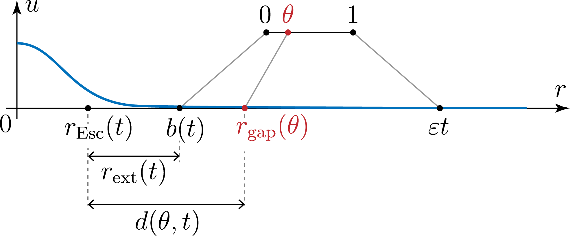
Figure 6.1: Illustration of the notation for the proof of conclusion 2 of Proposition 6.1.

Since $b(t)$ goes to $+\infty$ as $t$ goes to $+\infty$, it follows from the previous limit that

(6.33) $$\int_{0}^{b(t)}r^{d-1}E^{\dagger}(r,t)\,dr\to E[\phi]\quad\text{as}\quad t\to+\infty\,.$$

Let $\varepsilon$ denote a small positive quantity to be chosen below (the value of $\varepsilon$ is provided in 6.38 and depends only on $\phi$). According to conclusion 1 of Proposition 5.1,

(6.34) $$\int_{0}^{\varepsilon t}r^{d-1}E^{\dagger}(r,t)\,dr\to\mathcal{E}_{\textup{\text{res-asympt}}}[u]\quad\text{as}\quad t\to+\infty\,.$$

As a consequence, conclusion 2 of Proposition 6.1 is a consequence of the following lemma. ∎

Lemma 6.11 (the energy over the interval ${[}b(t),\varepsilon t{]}$ goes to $0$).

The following limit holds:

(6.35) $$\int_{b(t)}^{\varepsilon t}r^{d-1}E^{\dagger}(r,t)\,dr\to 0~\quad\text{as}\quad t\to+\infty\,.$$

Proof of Lemma 6.11.

According to the limits 6.7 and 6.31, $b^{\prime}(t)$ goes to $0$ as $t$ goes to $+\infty$. Thus there exists a time $t^{\prime}_{0}$ greater than or equal to $t_{0}$ such that, for every time $t$ greater than or equal to $t^{\prime}_{0}$, the quantity $b(t)$ is smaller than $\varepsilon t$. Let us call upon the notation $\kappa_{0}$ and $T_{\macc@depth\char 1\relax\frozen@everymath{\macc@group}\macc@set@skewchar\macc@nested@a 111{r}}\psi_{0}(r)$ and $\mathcal{F}_{0}(\macc@depth\char 1\relax\frozen@everymath{\macc@group}\macc@set@skewchar\macc@nested@a 111{r},t)$ and $\Sigma_{\textup{\text{Esc}},0}(t)$ and $\nu_{\mathcal{F}_{0}}$ and $K_{\mathcal{F}_{0}}$ introduced in 4.9, 4.12, 4.15, 4.23 and 4.25 (for the minimum point $m$ considered here), and let us introduce the functions $r_{\textup{\text{gap}}}$ and $\mathcal{G}$, defined on $[0,1]\times[t^{\prime}_{0},+\infty)$ with values in $[0,+\infty)$, defined as

(6.36) $$r_{\textup{\text{gap}}}(\theta,t)=(1-\theta)b(t)+\theta\varepsilon t\quad\text{and}\quad\mathcal{G}(\theta,t)=\mathcal{F}_{0}\bigl{(}r_{\textup{\text{gap}}}(\theta,t),t\bigr{)}\,,$$

see figure 6.1. For every $(\theta,t)$ in $[0,1]\times[t_{0},+\infty)$,

$$\partial_{t}\mathcal{G}(\theta,t)=\partial_{\macc@depth\char 1\relax\frozen@everymath{\macc@group}\macc@set@skewchar\macc@nested@a 111{r}}\mathcal{F}_{0}\bigl{(}r_{\textup{\text{gap}}}(\theta,t),t\bigr{)}\partial_{t}r_{\textup{\text{gap}}}(\theta,t)+\partial_{t}\mathcal{F}_{0}\bigl{(}r_{\textup{\text{gap}}}(\theta,t),t\bigr{)}\,.$$

According to inequality 4.19 of Lemma 4.3,

$$\partial_{t}\mathcal{F}_{0}\bigl{(}r_{\textup{\text{gap}}}(\theta,t),t\bigr{)} \leq-\nu_{\mathcal{F}_{0}}\mathcal{F}_{0}\bigl{(}r_{\textup{\text{gap}}}(\theta,t),t\bigr{)}+K_{\mathcal{F}_{0}}\int_{\Sigma_{\textup{\text{Esc}},0}(t)}T_{r_{\textup{\text{gap}}}(\theta,t)}\psi_{0}(r)\,dr$$

$$\leq-\nu_{\mathcal{F}_{0}}\mathcal{F}_{0}\bigl{(}r_{\textup{\text{gap}}}(\theta,t),t\bigr{)}+\frac{2K_{\mathcal{F}_{0}}}{\kappa_{0}}\exp\bigl{(}-\kappa_{0}d(\theta,t)\bigr{)}\,,$$

where $d(\theta,t)$ denotes the distance between $r_{\textup{\text{gap}}}(\theta,t)$ and the set $\Sigma_{\textup{\text{Esc}},0}(t)$ in $\mathbb{R}$. Let us assume that $\varepsilon$ is smaller than $c_{\textup{\text{hom}}}/2$ and, up to increasing $t^{\prime}_{0}$, let us assume that, for every time $t$ greater than or equal to $t^{\prime}_{0}$, the quantity $r_{\textup{\text{hom}}}(t)$ is not smaller than $2\varepsilon t$. Then, for every time $t$ greater than or equal to $t^{\prime}_{0}$,

(6.37) $$d(\theta,t)=r_{\textup{\text{gap}}}(\theta,t)-r_{\textup{\text{Esc}}}(t)\,,$$

see figure 6.1, and it follows from the previous inequality that

$$\partial_{t}\mathcal{F}_{0}\bigl{(}r_{\textup{\text{gap}}}(\theta,t),t\bigr{)}\leq-\nu_{\mathcal{F}_{0}}\mathcal{F}_{0}\bigl{(}r_{\textup{\text{gap}}}(\theta,t),t\bigr{)}+\frac{2K_{\mathcal{F}_{0}}}{\kappa_{0}}\exp\bigl{(}-\kappa_{0}d(\theta,t)\bigr{)}\,.$$

Besides, according to the definition 4.12 of the weight function $T_{\macc@depth\char 1\relax\frozen@everymath{\macc@group}\macc@set@skewchar\macc@nested@a 111{r}}\psi_{0}(\cdot)$,

$$\left\lvert\partial_{\macc@depth\char 1\relax\frozen@everymath{\macc@group}\macc@set@skewchar\macc@nested@a 111{r}}\mathcal{F}_{0}\bigl{(}r_{\textup{\text{gap}}}(\theta,t),t\bigr{)}\right\rvert\leq\kappa_{0}\mathcal{F}_{0}\bigl{(}r_{\textup{\text{gap}}}(\theta,t),t\bigr{)}$$

It follows that, for every time $t$ greater than or equal to $t^{\prime}_{0}$,

$$\partial_{t}\mathcal{G}(\theta,t)\leq-(\nu_{\mathcal{F}_{0}}-\varepsilon\kappa_{0})\mathcal{G}(\theta,t)+\frac{2K_{\mathcal{F}_{0}}}{\kappa_{0}}\exp\bigl{(}-\kappa_{0}d(\theta,t)\bigr{)}\,,$$

so that if the quantity $\varepsilon$ is chosen as

(6.38) $$\varepsilon=\min\left(\frac{c_{\textup{\text{hom}}}}{2},\frac{\nu_{\mathcal{F}_{0}}}{16\kappa_{0}}\right)\,,$$

then the previous inequality yields

(6.39) $$\partial_{t}\mathcal{G}(\theta,t)\leq-\frac{\nu_{\mathcal{F}_{0}}}{2}\mathcal{G}(\theta,t)+\frac{2K_{\mathcal{F}_{0}}}{\kappa_{0}}\exp\bigl{(}-\kappa_{0}d(\theta,t)\bigr{)}\,.$$

The factor $16$ in the denominator of the second quantity defining $\varepsilon$ will be useful for the next lemma, which, together with the forthcoming corollary, will complete the proof of Lemma 6.11. ∎

Lemma 6.12 (upper bound on $\mathcal{G}(\theta,t)$ for $t$ large positive).

There exists a time $t^{\prime\prime}_{0}$ greater than or equal to $t^{\prime}_{0}$ such that, for every $\theta$ in $[0,1]$ and every time $t$ greater than or equal to $t^{\prime\prime}_{0}$,

(6.40) $$\mathcal{G}(\theta,t)\leq\frac{8K_{\mathcal{F}_{0}}}{\kappa_{0}\nu_{\mathcal{F}_{0}}}\exp\bigl{(}-\kappa_{0}d(\theta,t)\bigr{)}\,.$$

Proof of Lemma 6.12.

Let us introduce the function $\mathcal{H}(\cdot,\cdot)$ defined as

(6.41) $$\mathcal{H}(\theta,t)=\mathcal{G}(\theta,t)-\frac{8K_{\mathcal{F}_{0}}}{\kappa_{0}\nu_{\mathcal{F}_{0}}}\exp\bigl{(}-\kappa_{0}d(\theta,t)\bigr{)}\,.$$

It follows from inequality 6.39 that, for every $\theta$ in $[0,1]$ and for every time $t$ greater than or equal to $t^{\prime}_{0}$,

$$\partial_{t}\mathcal{H}(\theta,t) \leq-\frac{\nu_{\mathcal{F}_{0}}}{2}\mathcal{G}(\theta,t)+\frac{2K_{\mathcal{F}_{0}}}{\kappa_{0}}\exp\bigl{(}-\kappa_{0}d(\theta,t)\bigr{)}+\frac{8K_{\mathcal{F}_{0}}}{\nu_{\mathcal{F}_{0}}}\partial_{t}d(\theta,t)\exp\bigl{(}-\kappa_{0}d(\theta,t)\bigr{)}$$

$$\leq-\frac{\nu_{\mathcal{F}_{0}}}{2}\mathcal{G}(\theta,t)+\frac{2K_{\mathcal{F}_{0}}}{\kappa_{0}}\exp\bigl{(}-\kappa_{0}d(\theta,t)\bigr{)}\left(1+\frac{4\kappa_{0}}{\nu_{\mathcal{F}_{0}}}\partial_{t}d(\theta,t)\right)$$

$$\leq-\frac{\nu_{\mathcal{F}_{0}}}{2}\mathcal{H}(\theta,t)-\frac{2K_{\mathcal{F}_{0}}}{\kappa_{0}}\exp\bigl{(}-\kappa_{0}d(\theta,t)\bigr{)}\left(1-\frac{4\kappa_{0}}{\nu_{\mathcal{F}_{0}}}\partial_{t}d(\theta,t)\right)\,.$$

According to the definitions 6.32, 6.36 and 6.37 of $b(t)$ and $r_{\textup{\text{gap}}}(t)$ and $d(\theta,t)$,

$$d(\theta,t)=(1-\theta)r_{\textup{\text{ext}}}(t)+\theta\bigl{(}\varepsilon t-r_{\textup{\text{Esc}}}(t)\bigr{)}\,,\quad\text{so that}\quad\partial_{t}d(\theta,t)=(1-\theta)r_{\textup{\text{ext}}}^{\prime}(t)+\theta\bigl{(}\varepsilon-r_{\textup{\text{Esc}}}^{\prime}(t)\bigr{)}\,.$$

Since $r_{\textup{\text{ext}}}^{\prime}(t)$ and $r_{\textup{\text{Esc}}}^{\prime}(t)$ go to $0$ as $t$ goes to $+\infty$, there exists a time $t^{\prime\prime\prime}_{0}$ greater than or equal to $t^{\prime}_{0}$ such that, if $t$ is greater than or equal to $t^{\prime\prime\prime}_{0}$, then

$$\partial_{t}d(\theta,t)\leq 2\varepsilon\,,\quad\text{thus}\quad\frac{4\kappa_{0}}{\nu_{\mathcal{F}_{0}}}\partial_{t}d(\theta,t)\leq\frac{1}{2}\,,$$

and as a consequence,

$$\partial_{t}\mathcal{H}(\theta,t) \leq-\frac{\nu_{\mathcal{F}_{0}}}{2}\mathcal{H}(\theta,t)-\frac{K_{\mathcal{F}_{0}}}{\kappa_{0}}\exp\bigl{(}-\kappa_{0}d(\theta,t)\bigr{)}$$

$$\leq-\frac{\nu_{\mathcal{F}_{0}}}{2}\mathcal{H}(\theta,t)-\frac{K_{\mathcal{F}_{0}}}{\kappa_{0}}\exp\bigl{(}-\kappa_{0}d(\theta,t^{\prime\prime\prime}_{0})\bigr{)}\exp\bigl{(}-2\varepsilon\kappa_{0}(t-t^{\prime\prime\prime}_{0})\bigr{)}\,.$$

Let us introduce the function $\mathcal{J}(\cdot,\cdot)$ defined as

$$\mathcal{J}(\theta,t)=\mathcal{H}(\theta,t)\exp\bigl{(}2\varepsilon\kappa_{0}(t-t^{\prime\prime\prime}_{0})\bigr{)}\,.$$

Then, if $t$ is greater than or equal to $t^{\prime\prime\prime}_{0}$,

$$\partial_{t}\mathcal{J}(\theta,t) \leq\Biggl{(}\biggl{(}-\frac{\nu_{\mathcal{F}_{0}}}{2}+2\varepsilon\kappa_{0}\biggr{)}\mathcal{H}(\theta,t)-\frac{K_{\mathcal{F}_{0}}}{\kappa_{0}}\exp\bigl{(}-\kappa_{0}d(\theta,t_{0}^{\prime\prime\prime})\bigr{)}\exp\bigl{(}-2\varepsilon\kappa_{0}(t-t_{0}^{\prime\prime\prime})\bigr{)}\Biggr{)}$$

$$\qquad\times\exp\bigl{(}2\varepsilon\kappa_{0}(t-t^{\prime\prime\prime}_{0})\bigr{)}$$

$$\leq-\frac{\nu_{\mathcal{F}_{0}}}{4}\mathcal{J}(\theta,t)-\frac{K_{\mathcal{F}_{0}}}{\kappa_{0}}\exp\bigl{(}-\kappa_{0}d(\theta,t_{0}^{\prime\prime\prime})\bigr{)}$$

$$\leq-\frac{\nu_{\mathcal{F}_{0}}}{4}\mathcal{J}(\theta,t)-\frac{K_{\mathcal{F}_{0}}}{\kappa_{0}}\exp\bigl{(}-\kappa_{0}d(1,t_{0}^{\prime\prime\prime})\bigr{)}\,.$$

This last inequality shows that $\mathcal{J}(\theta,t)$ must eventually become negative (and remain negative afterwards) as time increases. More precisely, since according to the bounds 3.1 on the solution the quantity $\mathcal{G}(\theta,t^{\prime\prime\prime}_{0})$ is bounded uniformly with respect to $\theta$, the same is true for the quantity $\mathcal{J}(\theta,t^{\prime\prime\prime}_{0})$. As a consequence, there must exist a time $t^{\prime\prime}_{0}$ greater than or equal to $t^{\prime\prime\prime}_{0}$ such that, for every $\theta$ in $[0,1]$ and every time $t$ greater than or equal to $t^{\prime\prime}_{0}$,

$$\mathcal{J}(\theta,t)\leq 0\,,\quad\text{so that}\quad\mathcal{H}(\theta,t)\leq 0\,,$$

and in view of the definition 6.41 of $\mathcal{H}(\theta,t)$, inequality 6.40 follows. Lemma 6.12 is proved. ∎

For every time $t$ greater than or equal to $t^{\prime}_{0}$, let us write

$$\mathcal{I}(t)=\int_{b(t)}^{\varepsilon t}{\macc@depth\char 1\relax\frozen@everymath{\macc@group}\macc@set@skewchar\macc@nested@a 111{r}}^{d-1}\mathcal{F}_{0}(\macc@depth\char 1\relax\frozen@everymath{\macc@group}\macc@set@skewchar\macc@nested@a 111{r},t)\,d\macc@depth\char 1\relax\frozen@everymath{\macc@group}\macc@set@skewchar\macc@nested@a 111{r}\,.$$

Corollary 6.13 ($\mathcal{I}(t)$ goes to $0$).

The quantity $\mathcal{I}(t)$ goes to $0$ as $t$ goes to $+\infty$.

Proof of Corollary 6.13.

For every time $t$ greater than or equal to $t^{\prime\prime}_{0}$, it follows from inequality 6.40 of Lemma 6.12 that, for every $\macc@depth\char 1\relax\frozen@everymath{\macc@group}\macc@set@skewchar\macc@nested@a 111{r}$ in $\bigl{[}b(t),\varepsilon t\bigr{]}$,

$$\mathcal{F}_{0}(\macc@depth\char 1\relax\frozen@everymath{\macc@group}\macc@set@skewchar\macc@nested@a 111{r},t)\leq\frac{8K_{\mathcal{F}_{0}}}{\kappa_{0}\nu_{\mathcal{F}_{0}}}\exp\Bigl{(}-\kappa_{0}\bigl{(}\macc@depth\char 1\relax\frozen@everymath{\macc@group}\macc@set@skewchar\macc@nested@a 111{r}-r_{\textup{\text{Esc}}}(t)\bigr{)}\Bigr{)}$$

so that

$$\mathcal{I}(t) \leq\frac{8K_{\mathcal{F}_{0}}}{\kappa_{0}\nu_{\mathcal{F}_{0}}}\exp\bigl{(}\kappa_{0}r_{\textup{\text{Esc}}}(t)\bigr{)}\int_{b(t)}^{\varepsilon t}{\macc@depth\char 1\relax\frozen@everymath{\macc@group}\macc@set@skewchar\macc@nested@a 111{r}}^{d-1}\exp(-\kappa_{0}\macc@depth\char 1\relax\frozen@everymath{\macc@group}\macc@set@skewchar\macc@nested@a 111{r})\,dr$$

$$\leq\frac{8K_{\mathcal{F}_{0}}}{\kappa_{0}\nu_{\mathcal{F}_{0}}}\exp\bigl{(}\kappa_{0}r_{\textup{\text{Esc}}}(t)\bigr{)}\frac{1}{\kappa_{0}^{d}}\int_{\kappa_{0}b(t)}^{+\infty}r^{d-1}e^{-r}\,dr$$

$$\leq\frac{8K_{\mathcal{F}_{0}}}{\kappa_{0}\nu_{\mathcal{F}_{0}}}\exp\bigl{(}\kappa_{0}r_{\textup{\text{Esc}}}(t)\bigr{)}\frac{(d-1)!}{\kappa_{0}^{d}}\exp\bigl{(}-\kappa_{0}b(t)\bigr{)}e_{d-1}\bigl{(}\kappa_{0}b(t)\bigr{)}\,,$$

where $e_{d-1}(\cdot)$ denotes the exponential sum function defined as

$$e_{d-1}(\tau)=\sum_{k=0}^{d-1}\frac{\tau^{k}}{k!}\,.$$

Since according to Lemma 6.10 the quantity $r_{\textup{\text{Esc}}}(t)$ converges as $t$ goes to $+\infty$, and since $b(t)$ goes to $+\infty$ as $t$ goes to $+\infty$, the intended limit follows. ∎

End of the proof of Lemma 6.11.

Let us assume that $t$ is positive large enough so that

(6.42) $$b(t)-1\geq r_{\textup{\text{s-c}}}\quad\text{and}\quad b(t)+1\leq\varepsilon t-1\,.$$

Then, according to the nonnegativity of $F^{\dagger}(r,t)$ (inequality 4.16), for every $\macc@depth\char 1\relax\frozen@everymath{\macc@group}\macc@set@skewchar\macc@nested@a 111{r}$ in $[b(t),\varepsilon t]$,

$$\mathcal{F}_{0}(\macc@depth\char 1\relax\frozen@everymath{\macc@group}\macc@set@skewchar\macc@nested@a 111{r},t)\geq\int_{\macc@depth\char 1\relax\frozen@everymath{\macc@group}\macc@set@skewchar\macc@nested@a 111{r}-1}^{\macc@depth\char 1\relax\frozen@everymath{\macc@group}\macc@set@skewchar\macc@nested@a 111{r}+1}T_{\macc@depth\char 1\relax\frozen@everymath{\macc@group}\macc@set@skewchar\macc@nested@a 111{r}}\psi_{0}(r)F^{\dagger}(r,t)\,dr\,,$$

so that, according to the definition 4.11 of $\psi_{0}$ and the first of the conditions 6.42,

$$\mathcal{F}_{0}(\macc@depth\char 1\relax\frozen@everymath{\macc@group}\macc@set@skewchar\macc@nested@a 111{r},t)\geq e^{-\kappa_{0}}\int_{\macc@depth\char 1\relax\frozen@everymath{\macc@group}\macc@set@skewchar\macc@nested@a 111{r}-1}^{\macc@depth\char 1\relax\frozen@everymath{\macc@group}\macc@set@skewchar\macc@nested@a 111{r}+1}F^{\dagger}(r,t)\,dr\,,$$

so that

$$\mathcal{I}(t) \geq e^{-\kappa_{0}}\int_{b(t)}^{\varepsilon t}{\macc@depth\char 1\relax\frozen@everymath{\macc@group}\macc@set@skewchar\macc@nested@a 111{r}}^{d-1}\left(\int_{\macc@depth\char 1\relax\frozen@everymath{\macc@group}\macc@set@skewchar\macc@nested@a 111{r}-1}^{\macc@depth\char 1\relax\frozen@everymath{\macc@group}\macc@set@skewchar\macc@nested@a 111{r}+1}F^{\dagger}(r,t)\,dr\right)\,d\macc@depth\char 1\relax\frozen@everymath{\macc@group}\macc@set@skewchar\macc@nested@a 111{r}$$

$$\geq e^{-\kappa_{0}}\left(\frac{b(t)}{b(t)-1}\right)^{d-1}\int_{b(t)}^{\varepsilon t}\left(\int_{\macc@depth\char 1\relax\frozen@everymath{\macc@group}\macc@set@skewchar\macc@nested@a 111{r}-1}^{\macc@depth\char 1\relax\frozen@everymath{\macc@group}\macc@set@skewchar\macc@nested@a 111{r}+1}r^{d-1}F^{\dagger}(r,t)\,dr\right)\,d\macc@depth\char 1\relax\frozen@everymath{\macc@group}\macc@set@skewchar\macc@nested@a 111{r}$$

$$=e^{-\kappa_{0}}\left(\frac{b(t)}{b(t)-1}\right)^{d-1}\int_{b(t)}^{\varepsilon t}r^{d-1}F^{\dagger}(r,t)\left(\int_{\max\bigl{(}r-1,b(t)\bigr{)}}^{\min\bigl{(}r+1,\varepsilon(t)\bigr{)}}\,d\macc@depth\char 1\relax\frozen@everymath{\macc@group}\macc@set@skewchar\macc@nested@a 111{r}\right)\,dr\,.$$

The quantity

$$\min\bigl{(}r+1,\varepsilon(t)\bigr{)}-\max\bigl{(}r-1,b(t)\bigr{)}=2+\min\bigl{(}r,\varepsilon(t)-1\bigr{)}-\max\bigl{(}r,b(t)+1\bigr{)}$$

is equal to

$$\left\{\begin{aligned} 1~+r-b(t)\quad&\text{if}\quad b(t)+1\leq r\leq\varepsilon t-1\,,\\ 2\quad&\text{if}\quad b(t)+1\leq r\leq\varepsilon t-1\,,\\ 1+\varepsilon t-r\quad&\text{if}\quad\varepsilon t-1\leq r\leq\varepsilon t\,,\end{aligned}\right.$$

and is therefore never less than $1$. It follows that

(6.43) $$\mathcal{I}(t)\geq e^{-\kappa_{0}}\left(\frac{b(t)}{b(t)-1}\right)^{d-1}\int_{b(t)}^{\varepsilon t}r^{d-1}F^{\dagger}(r,t)\,dr\,.$$

On the other hand, since the interval $\bigl{[}b(t),\varepsilon t\bigr{]}$ does not intersect the set $\Sigma_{\textup{\text{Esc}},0}(t)$, the following inequalities hold:

(6.44) $$\int_{b(t)}^{\varepsilon t}r^{d-1}F^{\dagger}(r,t)\,dr\geq\int_{b(t)}^{\varepsilon t}r^{d-1}E^{\dagger}(r,t)\,dr\geq 0\,:$$

The intended limit 6.35 follows from Corollary 6.13 and inequalities 6.43 and 6.44. Lemma 6.11 is proved. ∎

End of the proof of conclusion 2 of Proposition 6.1.

In view of the limits 6.33 and 6.34,conclusion 2 of Proposition 6.1 follows from Lemma 6.11 and is therefore proved. Since conclusion 6.1 of Proposition 6.1 was proved in subsection 6.3, the proof of Proposition 6.1 is complete. ∎

7 Proofs of Theorems 1, 2.6 and 2.7

Proof of Theorem 1.

Convergence towards the propagating terrace of bistable travelling fronts follows from Proposition 4.1, and the convergence towards a stationary solution behind these fronts follows from Proposition 6.1. The proof is the same as that of [54, Theorem 1] (see section 6 of this reference), thus details will not be reproduced here. ∎

Proof of Proposition 2.6.

This statement follows from conclusion 1 of Proposition 5.1 and from Proposition 6.1. ∎

Proof of Proposition 2.7.

The proof is very similar to the proof of [57, Corollary 10.2 and Corollary 10.4], see subsection 10.4 of this reference for details. The proof relies mainly on the upper semi-continuity of the asymptotic energy which is proved (in the broader setting of system 1.1 without the radial symmetry hypothesis) in [56] (see Proposition 2.9 of this reference). ∎

8 Spatial asymptotics for stationary solutions stable at the right end of space

Lemma 8.1 (spatial asymptotics for stationary solutions stable at the right end of space).

Let $m$ be a point of $\mathcal{M}$, let $\rho_{\textup{\text{left-end}}}$ be a quantity in $\{-\infty\}\cup(-\infty,0]$, let

$$I~=\left\{\begin{aligned} &[\rho_{\textup{\text{left-end}}},+\infty)\quad\text{if}\quad\rho_{\textup{\text{left-end}}}\in(-\infty,0]\,,\\ &(-\infty,+\infty)\quad\text{if}\quad\rho_{\textup{\text{left-end}}}=-\infty\,,\end{aligned}\right.$$

and let $\phi:I\to\mathbb{R}^{{d_{\textup{\text{st}}}}}$, $\rho\mapsto\phi(\rho)$ denote a function which is a solution:

(8.1) of system $$\phi^{\prime\prime}+\frac{d-1}{\rho-\rho_{\textup{\text{left-end}}}}\phi^{\prime}=\nabla V(\phi)$$

with the boundary condition $$\phi^{\prime}(\rho_{\textup{\text{left-end}}})=0\quad\text{if}\quad\rho_{\textup{\text{left-end}}}\in(-\infty,0]\,,$$

and of system $$\phi^{\prime\prime}=\nabla V(\phi)\quad\text{if}\quad\rho_{\textup{\text{left-end}}}=-\infty\,.$$

Assume that

(8.2) $$\left\lvert\phi(\rho)-m\right\rvert\leq\delta_{\textup{\text{Esc}}}(m)\quad\text{for every $\rho$ in $[0,+\infty)$}\quad\text{and}\quad\phi\not\equiv m\,.$$

Then the following conclusions hold.

1. Both quantities $\left\lvert\phi(\rho)-m\right\rvert$ and $\left\lvert\phi^{\prime}(\rho)\right\rvert$ go to $0$ as $\rho$ goes to $+\infty$.

2. For every $\rho$ in $[0,+\infty)$, the scalar product $\bigl{(}\phi(\rho)-m\bigr{)}\cdot\phi^{\prime}(\rho)$ is negative.

3. For every $\rho$ in $[0,+\infty)$, the quantity $\left\lvert\phi(\rho)-m\right\rvert$ is smaller than $\delta_{\textup{\text{Esc}}}(m)$.

4. The supremum $\sup_{\rho\in I}\left\lvert\phi(\rho)-m\right\rvert$ is larger than $\delta_{\textup{\text{Esc}}}(m)$.

Proof.

If $\rho_{\textup{\text{left-end}}}$ equals $-\infty$, then all conclusions follow from [54, Lemma 7.1]. Thus it may be assumed that $\rho_{\textup{\text{left-end}}}$ is in $(-\infty,0]$. Observe that the interval $[0,+\infty)$ is included in the interval $I$ where the function $\phi$ is defined. For every $\rho$ in $I$, let us introduce the quantities

(8.3) $$Q(\rho)=\frac{1}{2}\bigl{(}\phi(\rho)-m\bigr{)}^{2}\quad\text{and}\quad H(\rho)=\frac{1}{2}\phi^{\prime}(\rho)^{2}~-V\bigl{(}\phi(\rho)\bigr{)}\,.$$

Then, for all $\rho$ in $I$, it follows from system 8.1 that,

$$Q^{\prime}(\rho) =\bigl{(}\phi(\rho)-m\bigr{)}\cdot\phi^{\prime}(\rho)\,,$$

$$\text{and}\quad Q^{\prime\prime}(\rho) =\phi^{\prime}(\rho)^{2}+\bigl{(}\phi(\rho)-m\bigr{)}\cdot\nabla V\bigl{(}\phi(\rho)\bigr{)}-\frac{d-1}{\rho-\rho_{\textup{\text{left-end}}}}\bigl{(}\phi(\rho)-m\bigr{)}\cdot\phi^{\prime}(\rho)\,,$$

and thus, if $\rho$ is nonnegative, it follows from assumption 8.2 and from inequality 3.10 that

(8.4) $$Q^{\prime\prime}(\rho)\geq\phi^{\prime}(\rho)^{2}+\frac{\lambda_{\min}(m)}{2}\bigl{(}\phi(\rho)-m\bigr{)}^{2}-\frac{d-1}{\rho-\rho_{\textup{\text{left-end}}}}\bigl{(}\phi(\rho)-m\bigr{)}\cdot\phi^{\prime}(\rho)\,.$$

Let us introduce the quantity

$$\rho_{0}~=\rho_{\textup{\text{left-end}}}+(d-1)\sqrt{\frac{2}{\lambda_{\min}(m)}}\,.$$

For every $\rho$ greater than or equal to $\rho_{0}$,

$$\left\lvert\frac{d-1}{\rho-\rho_{\textup{\text{left-end}}}}\bigl{(}\phi(\rho)-m\bigr{)}\cdot\phi^{\prime}(\rho)\right\rvert \leq\frac{1}{2}\phi^{\prime}(\rho)^{2}+\frac{1}{2}\left(\frac{d-1}{\rho-\rho_{\textup{\text{left-end}}}}\right)^{2}\bigl{(}\phi(\rho)-m\bigr{)}^{2}~$$

$$\leq\frac{1}{2}\phi^{\prime}(\rho)^{2}+\frac{\lambda_{\min}(m)}{4}\bigl{(}\phi(\rho)-m\bigr{)}^{2}\,,$$

so that, for every $\rho$ greater than or equal to $\max(0,\rho_{0})$, it follows from 8.4 that

(8.5) $$Q^{\prime\prime}(\rho)\geq\frac{1}{2}\phi^{\prime}(\rho)^{2}+\frac{\lambda_{\min}(m)}{4}\bigl{(}\phi(\rho)-m\bigr{)}^{2}\,.$$

On the other hand, it again follows from system 8.1 that, for all $\rho$ in $I$,

(8.6) $$H^{\prime}(\rho)=-\frac{d-1}{\rho-\rho_{\textup{\text{left-end}}}}\phi^{\prime}(\rho)^{2}\,,$$

thus the function $H(\cdot)$ is non-increasing and thus bounded from above on $I$, and it follows from assumption 8.2 that $V\bigl{(}\phi(\cdot)\bigr{)}$ is bounded on $[0,+\infty)$. According to the expression 8.3 of $H(\cdot)$, it follows that $\phi^{\prime}(\cdot)$ is bounded on $[0,+\infty)$, so that $Q^{\prime}(\cdot)$ is bounded on $I$. Since according to inequality 8.5 the function $Q^{\prime}(\cdot)$ is non-decreasing (and even strictly increasing since $\phi$ is not identically equal to $m$) on $\bigl{[}\max(0,\rho_{0}),+\infty\bigr{)}$, it follows that $Q^{\prime}(\rho)$ must converge towards a finite limit as $\rho$ goes to $+\infty$; and thus it follows from inequality 8.5 that both functions $\phi^{\prime}(\cdot)^{2}$ and $Q(\cdot)$ are square-integrable on $I$. Since $Q^{\prime}(\cdot)$ is bounded, it follows that $Q(\rho)$ must converge towards $0$ as $\rho$ goes to $+\infty$. Thus $\phi(\rho)$ goes to $m$ as $\rho$ goes to $+\infty$, and as a consequence $V\bigl{(}\phi(\rho)\big{)}$ goes to $V(m)$ as $\rho$ goes to $+\infty$. Thus, since the function $H(\cdot)$ must converge to a finite limit at $+\infty$, it follows that $\phi^{\prime}(\rho)^{2}$ must also go to a finite limit when $\rho$ goes to $+\infty$. Since $\phi^{\prime}(\cdot)^{2}$ is integrable on $I$, its limit at $+\infty$ must be $0$. Assertion 1 is proved.

It follows from assertion 1 that $Q^{\prime}(\cdot)$ converges towards $0$ at $+\infty$, thus since this function is strictly increasing on $\bigl{[}\max(0,\rho_{0}),+\infty\bigr{)}$, it follows that $Q^{\prime}(\rho)$ is negative for all $\rho$ in this interval. To prove assertion 2, let us proceed by contradiction and assume that $Q^{\prime}(\cdot)$ takes a nonnegative value somewhere in $I$. Then $\rho_{0}$ must be larger than $\rho_{\textup{\text{left-end}}}$, and $Q^{\prime}(\cdot)$ must takes a nonnegative value somewhere in $[\rho_{\textup{\text{left-end}}},\rho_{0})$. Let

$$\rho_{1}=\max\{\rho\in[\rho_{\textup{\text{left-end}}},\rho_{0}):Q^{\prime}(\rho)\geq 0\}\,.$$

Then $Q^{\prime}(\cdot)$ is negative on $(\rho_{1},+\infty)$ and it follows from 8.4 that $Q^{\prime\prime}(\cdot)$ is positive on this interval, thus $Q^{\prime}(\cdot)$ is strictly increasing on this interval, and it follows that $Q^{\prime}(\rho_{1})$ is negative, a contradiction with the definition of $\rho_{1}$. Assertion 2 is proved, and assertion 3 follows from assertion 2. Since according to the boundary condition 8.1 the scalar product $\bigl{(}\phi(\rho_{\textup{\text{left-end}}})-m\bigr{)}\cdot\phi^{\prime}(\rho_{\textup{\text{left-end}}})$ must be equal to $0$, it follows from assertion 2 that $\rho_{\textup{\text{left-end}}}$ cannot be equal to $0$, or equivalently that assumption 8.2 cannot hold up to $\rho_{\textup{\text{left-end}}}$, and this proves assertion 4. Lemma 8.1 is proved. ∎

Acknowledgements

I am indebted to Thierry Gallay and Romain Joly for their help and interest through numerous fruitful discussions.

Emmanuel Risler
Université de Lyon, INSA de Lyon, CNRS UMR 5208, Institut Camille Jordan,
F-69621 Villeurbanne, France.
emmanuel.risler@insa-lyon.fr

References

- [1] Nicholas D. Alikakos, Giorgio Fusco and Panayotis Smyrnelis “Elliptic Systems of Phase Transition Type” 91, Progress in Nonlinear Differential Equations and Their Applications Cham: Springer International Publishing, 2018 DOI: 10.1007/978-3-319-90572-3
- [2] Nicholas D. Alikakos and Nikolaos I. Katzourakis “Heteroclinic travelling waves of gradient diffusion systems” In Trans. Am. Math. Soc. 363.03, 2011, pp. 1365–1365 DOI: 10.1090/S0002-9947-2010-04987-6
- [3] D.. Aronson and H.. Weinberger “Multidimensional nonlinear diffusion arising in population genetics” In Adv. Math. (N. Y). 30.1, 1978, pp. 33–76 DOI: 10.1016/0001-8708(78)90130-5
- [4] H. Berestycki and P.. Lions “Nonlinear scalar field equations, I existence of a ground state” In Arch. Ration. Mech. Anal. 82.4, 1983, pp. 313–345 DOI: 10.1007/BF00250555
- [5] Henri Berestycki, Pierre Louis Lions and Lambertus A. Peletier “An ODE Approach to the Existence of Positive Solutions for Semilinear Problems in ” In Indiana Univ. Math. J., 1981, pp. 141–157
- [6] Juliette Bouhours and Thomas Giletti “Extinction and spreading of a species under the joint influence of climate change and a weak Allee effect: a two-patch model” In arXiv, 2016, pp. 1–33 arXiv: http://arxiv.org/abs/1601.06589
- [7] Juliette Bouhours and Thomas Giletti “Spreading and Vanishing for a Monostable Reaction – Diffusion Equation with Forced Speed” In J. Dyn. Differ. Equations Springer US, 2018 DOI: 10.1007/s10884-018-9643-5
- [8] Juliette Bouhours and Grégroie Nadin “A variational approach to reaction-diffusion equations with forced speed in dimension 1” In Discret. Contin. Dyn. Syst. - A 35.5, 2015, pp. 1843–1872 DOI: 10.3934/dcds.2015.35.1843
- [9] Guillemette Chapuisat “Existence and nonexistence of curved front solution of a biological equation” In J. Differ. Equ. 236.1, 2007, pp. 237–279 DOI: 10.1016/j.jde.2007.01.021
- [10] Guillemette Chapuisat and Romain Joly “Asymptotic profiles for a travelling front solution of a biological equation” In Math. Model. Methods Appl. Sci. 21.10, 2011, pp. 2155–2177 DOI: 10.1142/S0218202511005696
- [11] Chao-Nien Chen and Vittorio Coti Zelati “Traveling wave solutions to the Allen–Cahn equation” In Ann. l’Institut Henri Poincaré C, Anal. non linéaire 39, 2022, pp. 905–926 DOI: 10.4171/aihpc/23
- [12] Chiun Chuan Chen, Hung Yu Chien and Chih Chiang Huang “A variational approach to three-phase traveling waves for a gradient system” In Discret. Contin. Dyn. Syst. Ser. A 41.10, 2021, pp. 4737–4765 DOI: 10.3934/dcds.2021055
- [13] Yihong Du and Hiroshi Matano “Convergence and sharp thresholds for propagation in nonlinear diffusion problems” In J. Eur. Math. Soc. 12.2, 2010, pp. 279–312 DOI: 10.4171/JEMS/198
- [14] Yihong Du and Hiroshi Matano “Radial terrace solutions and propagation profile of multistable reaction-diffusion equations over ” In arXiv, 2020, pp. 4–21 arXiv: http://arxiv.org/abs/1711.00952
- [15] Yihong Du and Peter Polacik “Locally uniform convergence to an equilibrium for nonlinear parabolic equations on ” In Indiana Univ. Math. J. 64.3, 2015, pp. 787–824 DOI: 10.1512/iumj.2015.64.5535
- [16] Arnaud Ducrot, Thomas Giletti and Hiroshi Matano “Existence and convergence to a propagating terrace in one-dimensional reaction-diffusion equations” In Trans. Am. Math. Soc. 366.10, 2014, pp. 5541–5566 DOI: 10.1090/S0002-9947-2014-06105-9
- [17] Paul C. Fife and John Bryce McLeod “The approach of solutions of nonlinear diffusion equations to travelling front solutions” In Arch. Ration. Mech. Anal. 65.4, 1977, pp. 335–361 DOI: 10.1007/BF00250432
- [18] Paul C. Fife and John Bryce McLeod “A phase plane discussion of convergence to travelling fronts for nonlinear diffusion” In Arch. Ration. Mech. Anal. 75.4, 1981, pp. 281–314 DOI: 10.1007/BF00256381
- [19] PaulC. Fife “Long time behavior of solutions of bistable nonlinear diffusion equations” In Arch. Ration. Mech. Anal. 70.1, 1979, pp. 31–36 DOI: 10.1007/BF00276380
- [20] Thierry Gallay and Romain Joly “Global stability of travelling fronts for a damped wave equation with bistable nonlinearity” In Ann. Sci. l’École Norm. Supérieure 42.1, 2009, pp. 103–140 DOI: 10.24033/asens.2091
- [21] Thierry Gallay and Emmanuel Risler “A variational proof of global stability for bistable travelling waves” In Differ. Integr. Equations 20.8, 2007, pp. 901–926 arXiv: http://arxiv.org/abs/math/0612684%20http://projecteuclid.org/euclid.die/1356039363
- [22] Thomas Giletti and Hiroshi Matano “Existence and uniqueness of propagating terraces” In Commun. Contemp. Math. 22.06, 2020, pp. 1950055 DOI: 10.1142/S021919971950055X
- [23] Thomas Giletti and Luca Rossi “Pulsating solutions for multidimensional bistable and multistable equations” In Math. Ann. 378.3-4 Springer Berlin Heidelberg, 2020, pp. 1555–1611 DOI: 10.1007/s00208-019-01919-z
- [24] François Hamel and Luca Rossi “Spreading speeds and one-dimensional symmetry for reaction-diffusion equations” In arXiv, 2021, pp. 1–88 arXiv: http://arxiv.org/abs/2105.08344
- [25] Steffen Heinze “A variational approach to travelling waves”, 2001
- [26] Daniel B. Henry “Geometric Theory of Semilinear Parabolic Equations” In Lect. notes Math. 840, Lecture Notes in Mathematics Berlin, New-York: Springer Berlin Heidelberg, 1981 DOI: 10.1007/BFb0089647
- [27] Romain Joly and Emmanuel Risler “Generic transversality of travelling fronts, standing fronts, and standing pulses for parabolic gradient systems” In arXiv, 2023 arXiv: http://arxiv.org/abs/2301.02095
- [28] Christopher K… Jones “Asymptotic behavior of a reaction-diffusion equation in higher space dimensions” In Rocky Mt. J. Math. 13.2, 1983, pp. 355–364 DOI: 10.1216/RMJ-1983-13-2-355
- [29] Christopher K… Jones “Spherically symmetric solutions of a reaction-diffusion equation” In J. Differ. Equ. 49.1, 1983, pp. 142–169 DOI: 10.1016/0022-0396(83)90023-2
- [30] Cao Luo “Global stability of travelling fronts for a damped wave equation” In J. Math. Anal. Appl. 399 Elsevier Ltd, 2013, pp. 260–278 DOI: 10.1016/j.jmaa.2012.05.089
- [31] H. Matano and P. Poláčik “Dynamics of nonnegative solutions of one-dimensional reaction–diffusion equations with localized initial data. Part I: A general quasiconvergence theorem and its consequences” In Commun. Partial Differ. Equations 41.5, 2016, pp. 785–811 DOI: 10.1080/03605302.2016.1156697
- [32] H. Matano and P. Poláčik “An entire solution of a bistable parabolic equation on R with two colliding pulses” In J. Funct. Anal. 272.5 Elsevier Inc., 2017, pp. 1956–1979 DOI: 10.1016/j.jfa.2016.11.006
- [33] H. Matano and P. Poláčik “Dynamics of nonnegative solutions of one-dimensional reaction-diffusion equations with localized initial data. Part II: Generic nonlinearities” In Commun. Partial Differ. Equations 45.6, 2020, pp. 483–524 DOI: 10.1080/03605302.2019.1700273
- [34] Hiroshi Matano, Yoichiro Mori and Mitsunori Nara “Asymptotic behavior of spreading fronts in the anisotropic Allen–Cahn equation on ” In Ann. l’Institut Henri Poincaré C, Anal. non linéaire 36.3, 2019, pp. 585–626 DOI: 10.1016/j.anihpc.2018.07.003
- [35] Hiroshi Matsuzawa and Mitsunori Nara “Asymptotic behavior of spreading fronts in an anisotropic multi-stable equation on ” In Discret. Contin. Dyn. Syst., 2022, pp. 1–34 DOI: 10.3934/dcds.2022069
- [36] Cyrill B. Muratov “A global variational structure and propagation of disturbances in reaction-diffusion systems of gradient type” In Discret. Contin. Dyn. Syst. - Ser. B 4.4, 2004, pp. 867–892 DOI: 10.3934/dcdsb.2004.4.867
- [37] Cyrill B. Muratov and M Novaga “Front propagation in infinite cylinders. I. A variational approach” In Commun. Math. Sci. 6.4, 2008, pp. 799–826 DOI: 10.4310/CMS.2008.v6.n4.a1
- [38] Cyrill B. Muratov and M. Novaga “Front propagation in infinite cylinders. II. The sharp reaction zone limit” In Calc. Var. Partial Differ. Equ. 31.4, 2008, pp. 521–547 DOI: 10.1007/s00526-007-0125-6
- [39] Cyrill B. Muratov and M. Novaga “Global exponential convergence to variational traveling waves in cylinders” In SIAM J. Math. Anal. 44.1, 2012, pp. 293–315 DOI: 10.1137/110833269
- [40] Cyrill B. Muratov and X. Zhong “Threshold phenomena for symmetric decreasing solutions of reaction-diffusion equations” In Nonlinear Differ. Equations Appl. NoDEA 20.4, 2013, pp. 1519–1552 DOI: 10.1007/s00030-013-0220-7
- [41] Cyrill B. Muratov and Xing Zhong “Threshold phenomena for symmetric-decreasing radial solutions of reaction-diffusion equations” In Discret. Contin. Dyn. Syst. Ser. A 37.2, 2017, pp. 915–944 DOI: 10.3934/dcds.2017038
- [42] Ramon Oliver-Bonafoux “Heteroclinic traveling waves of 1D parabolic systems with degenerate stable states” In arXiv, 2021, pp. 1–37 arXiv: http://arxiv.org/abs/2111.12546
- [43] Ramon Oliver-Bonafoux “Heteroclinic traveling waves of 2D parabolic Allen-Cahn systems” In arXiv, 2021, pp. 1–67 arXiv: http://arxiv.org/abs/2106.09441
- [44] Ramon Oliver-Bonafoux and Emmanuel Risler “Global convergence towards pushed travelling fronts for parabolic gradient systems” In arXiv, 2023 arXiv: http://arxiv.org/abs/2306.04413
- [45] Antoine Pauthier, Jens D M Rademacher and Dennis Ulbrich “Weak and Strong Interaction of Excitation Kinks in Scalar Parabolic Equations” In J. Dyn. Differ. Equations Springer US, 2021 DOI: 10.1007/s10884-021-10040-2
- [46] Stanislav Ivanovich Pokhozhaev “On the eigenfunctions of the equation ” In Dokl. Akad. Nauk SSSR 165, 1965, pp. 36–39
- [47] Peter Poláčik “Propagating terraces in a proof of the Gibbons conjecture and related results” In J. Fixed Point Theory Appl., 2016, pp. 1–21 DOI: 10.1007/s11784-016-0343-7
- [48] Peter Poláčik “Convergence and Quasiconvergence Properties of Solutions of Parabolic Equations on the Real Line: An Overview” In Patterns Dyn. Springer, Cham, 2017, pp. 172–183 DOI: 10.1007/978-3-319-64173-7_11
- [49] Peter Poláčik “Planar Propagating Terraces and the Asymptotic One-dimensional Symmetry of Solutions of Semilinear Parabolic Equations” In SIAM J. Math. Anal. 49.5, 2017, pp. 3716–3740 DOI: 10.1137/16M1100745
- [50] Peter Poláčik “Propagating Terraces and the Dynamics of Front-Like Solutions of Reaction-Diffusion Equations on R” In Mem. Am. Math. Soc. 264.1278, 2020, pp. 1–100 DOI: 10.1090/memo/1278
- [51] Peter Poláčik “On bounded radial solutions of parabolic equations on : Quasiconvergence for initial data with a stable limit at infinity (preprint)”, 2023, pp. 1–23
- [52] Emmanuel Risler “Global convergence toward traveling fronts in nonlinear parabolic systems with a gradient structure” In Ann. l’Institut Henri Poincare. Ann. Anal. Non Lineaire/Nonlinear Anal. 25.2, 2008, pp. 381–424 DOI: 10.1016/j.anihpc.2006.12.005
- [53] Emmanuel Risler “Generic transversality of radially symmetric stationary solutions stable at infinity for parabolic gradient systems” In arXiv, 2023 arXiv:2301.02605
- [54] Emmanuel Risler “Global behaviour of bistable solutions for gradient systems in one unbounded spatial dimension” In arXiv, 2023 arXiv: http://arxiv.org/abs/1604.02002
- [55] Emmanuel Risler “Global behaviour of bistable solutions for hyperbolic gradient systems in one unbounded spatial dimension” In arXiv, 2023 arXiv: https://arxiv.org/abs/1703.01221
- [56] Emmanuel Risler “Global behaviour of solutions stable at infinity for gradient systems in higher space dimension: the no invasion case” In arXiv, 2023 arXiv: http://arxiv.org/abs/2206.06288
- [57] Emmanuel Risler “Global relaxation of bistable solutions for gradient systems in one unbounded spatial dimension” In arXiv, 2023 arXiv: http://arxiv.org/abs/1604.00804
- [58] Jean-Michel Roquejoffre and Violaine Roussier-Michon “Sharp large time behaviour in -dimensional reaction-diffusion equations of bistable type” In arXiv, 2021, pp. 1–15 arXiv: http://arxiv.org/abs/2101.07333
- [59] Violaine Roussier-Michon “Stability of radially symmetric travelling waves in reaction–diffusion equations” In Ann. l’Institut Henri Poincare Non Linear Anal. 21.3, 2004, pp. 341–379 DOI: 10.1016/j.anihpc.2003.04.002
- [60] Kohei Uchiyama “Asymptotic behavior of solutions of reaction-diffusion equations with varying drift coefficients” In Arch. Ration. Mech. Anal. 90.4, 1985, pp. 291–311 DOI: 10.1007/BF00276293
- [61] Andrej Zlatoš “Sharp transition between extinction and propagation of reaction” In J. Am. Math. Soc. 19.1, 2005, pp. 251–263 DOI: 10.1090/S0894-0347-05-00504-7