Using angular pair upweighting to improve 3D clustering measurements

Abstract

Three dimensional galaxy clustering measurements provide a wealth of cosmological information. However, obtaining spectra of galaxies is expensive, and surveys often only measure redshifts for a subsample of a target galaxy population. Provided that the spectroscopic data is representative, we argue that angular pair upweighting should be used in these situations to improve the 3D clustering measurements. We present a toy model showing mathematically how such a weighting can improve measurements, and provide a practical example of its application using mocks created for the Baryon Oscillation Spectroscopic Survey (BOSS). Our analysis of mocks suggests that, if an angular clustering measurement is available over twice the area covered spectroscopically, weighting gives a $\sim$10–20% reduction of the variance of the monopole correlation function on the BAO scale.

1 Introduction

The recent cosmological measurements of the Baryon Acoustic Oscillation (BAO) at the percent level, and measurements of the Redshift-Space Distortion (RSD) signals at the few percent level, in the clustering of galaxies selected from the Baryon Oscillation Spectroscopic Survey (BOSS; Dawson et al. 2013), part of the Sloan Digital Sky Survey III (Eisenstein et al., 2011), have clearly demonstrated the power of such measurements to understand the low-redshift Universe (Alam et al., 2016). Over the next decade, surveys including eBOSS (Dawson et al., 2016), DESI (Amir et al., 2016a, b), and Euclid (Laureijs, 2011), will provide an order of magnitude improvement on these constraints, helping us to understand Dark Energy.

Given the significant investment in these spectroscopic surveys, it is imperative to extract as much information as possible from them. One avenue that has been relatively unexploited until now is the possibility of using extended target sample data to enhance the spectroscopic measurements of a subset of it. It is common to be in the position of only having spectroscopic data for a subsample of targets. For example, the VIMOS Public Extragalactic Redshift Survey (VIPERS; Guzzo et al. 2014) spectroscopically observed $24$ deg² of the $157$ deg² Canada-France-Hawaii Telescope Legacy Survey (CFHTLS) Wide photometric catalogue. Similarly, the BOSS DR9 analyses presented in Anderson et al. (2012) used $3,275$ deg² of spectroscopic data, out of a target sample covering $9,274$ deg². An obvious question is “how best to use the extra target data to enhance the 3D clustering measurements?”. We argue here that angular pair upweighting does this.

Angular pair upweighting has previously been used to partially correct for spectroscopic completeness. It was used in Hawkins et al. (2003) to correct for missing close pairs in the 2dFGRS (Colless et al., 2003). It was also used in recent analyses of the VIPERS data: the pattern of observations allowed by the VIMOS instrument meant that the VIPERS galaxy clustering signal was strongly distorted by the spectroscopic completeness. de la Torre et al. (2013) and de la Torre et al. (2016) used angular pair weighted to correct for the incompletenesses, weighting pairs counted in a 3D correlation function measurement by the ratio $(1+w_{p}(\theta))/(1+w_{s}(\theta))$, where $w(\theta)$ is the angular correlation function, subscript $s$ denotes the spectroscopic sample, and $p$ the photometric sample.

We investigate the utility of angular pair upweighting, not to correct for missing observations, but to improve on 3D clustering measurements. In our companion paper (Bianchi & Percival, 2017) we present a new scheme to de-bias measurements from the effects of systematically missing observations, showing that angular pair upweighting alone only partially alleviates the effects. However, in Bianchi & Percival (2017), we argue that if forms part of a more complicated scheme to correct for missing observations that uses angular pair upweighting to recoup lost signal-to-noise. The investigation described here shows that it has the potential for wider application in the analysis of spectroscopic galaxy surveys.

In Section 2, we present a toy analytic model for angular pair upweighting, for the simple situation of uncorrelated 3D pair measurements in a single bin in $r$ and $\theta$. This is extended to correlated pairs in Section 3. In Section 4 we present an analysis of mock catalogues designed to match the DR12 BOSS sample, showing how angular clustering measurements from a wide area can enhance 3D clustering measurements. Our results are discussed in Section 5.

2 Uncorrelated pair counts

We first present an analytic toy model demonstrating the basic idea of pair upweighting. We have matched the notation of Landy & Szalay (1993), so we can use their method for describing pair counts within surveys, and our equations can be directly compared to theirs.

Consider $n_{g}$ objects angularly distributed within a region $\Omega$ with dimensionless geometric form factor $G_{p}(\theta)$, which encodes the geometry of the survey (as in Landy & Szalay 1993) as a distribution of pairs separated by $\theta\pm\Delta\theta/2$. Now consider a representative sample of galaxies that have spectroscopic data, denoted with a subscript $1$. For Poisson distributed pairs, the expected number in an angular bin is given by,

$$N_{p,1}\equiv\langle n_{p,1}\rangle=\frac{n_{g,1}(n_{g,1}-1)}{2}G_{p,1}(\theta).$$ (1)

Given spectroscopic information, suppose that $m_{p,1}$ of these are placed in the radial bin $r\pm\Delta r/2$ with selection probability $G_{r}(r|\theta)$. For the selection probability, we drop the subscript $1$ as we assume that this sample has representative selection. We have from Bayes theorem that

$$P(m_{p,1})=\int\,dn_{p,1}\,P(m_{p,1}|n_{p,1})P(n_{p,1}).$$ (2)

For uncorrelated pair counts, $m_{p,1}\sim B(n_{p,1},G_{r}(r|\theta))$ has a Binomial distribution. In order to avoid problems later if we had zero pairs in an angular bin (we need at least one pair in each angular bin, to be able to divide by the observed pair counts), we assume that $n_{p,1}$ is drawn from a zero-truncated Poisson distribution, rather than a Poisson distribution, so that

$$P(n_{p,1}=k|n_{p,1}>1)=\frac{N_{p,1}^{k}}{(e^{N_{p,1}}-1)k!},$$ (3)

and the expected number of pairs is slightly changed,

$$\langle n_{p,1}\rangle=\frac{N_{p,1}e^{N_{p,1}}}{e^{N_{p,1}}-1}.$$ (4)

Using a zero-truncated Poisson distribution rather than a Poisson distribution is simply a mathematical convenience, as we will only be concerned with the situation where $N_{p,1}$ is large. Using Eq. (2) to solve for the mean and variance of $m_{p,1}$ gives that

$$\langle m_{p,1}\rangle=\frac{N_{p,1}G_{r}}{1-e^{-N_{p,1}}},$$ (5)

and

$${\rm Var}(m_{p,1})=\frac{N_{p,1}G_{r}+N^{2}_{p,1}G^{2}_{r}}{1-e^{-N_{p,1}}}-\frac{N^{2}_{p,1}G^{2}_{r}}{(1-e^{-N_{p,1}})^{2}},$$ (6)

where we have written $G_{r}=G_{r}(r|\theta)$ for simplicity. In the limit of large $N_{p,1}$, this reduces to the standard Poisson result of both the mean and variance equalling $N_{p,1}G_{r}$. Here, when calculating the variance, we have ignored the effect of triplets, as considered, for example, in Landy & Szalay (1993), and assume that the dominant error term is Poisson.

Now suppose that we introduce angular sample $2$ for which we do not have radial information, but that has clustering that is statistically identical to that of sample $1$. For our toy model, we assume that $n_{p,2}$ is drawn from a zero-truncated Poisson distribution, that is independent of $n_{p,1}$ and has a probability density function as in Eq. (3), but with parameter $N_{p,2}$ rather than $N_{p,1}$. We will construct our estimator by combining both samples, so that we now have

$$P(\tilde{m}_{p,1})=\int\,dn_{p,1}\,dn_{p,2}\,P(\tilde{m}_{p,1}|n_{p,1},n_{p,2})P(n_{p,1})P(n_{p,2}).$$ (7)

We wish to use the combined information from both samples to form a maximum likelihood estimator for the expected number of angular pairs in sample $1$. Provided that $G_{p,1}(\theta)$ and $G_{p,2}(\theta)$ have similar distributions, then we can construct this by simply summing the regions together

$$\tilde{n}_{p,1}\equiv\frac{A_{1}(n_{p,1}+n_{p,2})}{A_{1}+A_{2}},$$ (8)

where $A_{1}$ and $A_{2}$ are the relative areas covered by samples $1$ and $2$ respectively. Angular pair upweighting treats $\tilde{n}_{p,1}/n_{p,1}$ as a weight to be applied to $m_{p,1}$ to give $\tilde{m}_{p,1}$

$$\tilde{m}_{p,1}=\frac{A_{1}(n_{p,1}+n_{p,2})}{n_{p,1}(A_{1}+A_{2})}m_{p,1},$$ (9)

and we see that the mean is unchanged. i.e.

$$\langle\tilde{m}_{p,1}\rangle=\frac{N_{p,1}G_{r}}{1-e^{-N_{p,1}}}.$$ (10)

Working in the limit where $N_{p,1}$ and $N_{p,2}$ are large so that $\langle 1/N_{p,1}\rangle\simeq 1/\langle N_{p,1}\rangle$, $e^{-N_{p,1}}\to 0$ and $e^{-N_{p,2}}\to 0$, the variance is changed to

$${\rm Var}(\tilde{m}_{p,1})=\frac{A_{1}^{2}G_{r}}{(A_{1}+A_{2})^{2}}\Bigg{[}N_{p,1}+N_{p,2}G_{r}+$$

$$\left(2N_{p,2}+\frac{N_{p,2}}{N_{p,1}}+\frac{N^{2}_{p,2}}{N_{p,1}}\right)(1-G_{r})\Bigg{]}.$$ (11)

Taking the limit of large $N_{p,1}$, and rewriting areas in terms of $N_{p,1}$ and $N_{p,2}$, the difference between this and the original variance reduces to the simple form

$$\frac{N_{p,1}G_{r}-{\rm Var}(\tilde{m}_{p,1})}{N_{p,1}G_{r}}=\frac{G_{r}}{1+N_{p,1}/N_{p,2}},$$ (12)

and we clearly see that ${\rm Var}(\tilde{m}_{p,1})<{\rm Var}(m_{p,1})$ for all $N_{p,2}>0$. The numerator of $G_{r}$ in Eq. (12) shows that the improvement in the variance is proportional to the fraction of pairs entering each radial bin. The denominator shows that the limiting maximum fractional improvement, which equals $G_{r}$, is logarithmically reached in the limit of large $N_{p,2}/N_{p,1}$.

3 Correlated pair counts

The relation between the 3D correlation function and its angular and radial components can be written

$$1+\xi(r,\theta)=(1+\xi(r|\theta))(1+w(\theta)),$$ (13)

where $w(\theta)$ is the angular correlation function, and $\xi(r|\theta)$ is the radial correlation function for pairs within this angular bin. As explained in Landy & Szalay (1993), because our sample geometry limits the distribution of pairs in both angular and radial directions, the relation between the measured clustering and the true correlation function requires an “Integral Constraint”. Thus, with clustering, Eq. 1 becomes

$$N_{p,1}=\frac{n_{g,1}(n_{g,1}-1)}{2}G_{p,1}(\theta)\frac{1+w(\theta)}{1+w_{\Omega}},$$ (14)

where

$$1+w_{\Omega}=\int_{\Omega}\,d\Omega\,G_{p,1}(\theta)(1+w(\theta)).$$ (15)

Similarly in the radial direction, Eq. (5) becomes

$$\langle m_{p,1}\rangle=\frac{N_{p,1}G_{r}(r|\theta)(1+\xi(r|\theta))}{(1+\xi_{r})(1-e^{-N_{p,1}})},$$ (16)

where

$$1+\xi_{r}=\int_{r}\,dr\,G_{r}(r|\theta)(1+\xi(r|\theta).$$ (17)

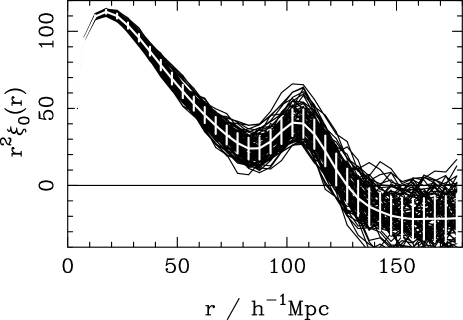
Figure 1: Monopole moments of the correlation function rebinned into bins of width $\Delta r=5.5\,h^{-1}\,{\rm Mpc}$, calculated from 100 of the 1000 QPM mocks used, matching the NGP component of the DR12 BOSS CMASS sample (black lines). The overplotted white line shows the mean, with 1$\sigma$ errors.

Thus we see that the effect of clustering, including both the correlation functions and integral constraints, can be absorbed into the geometric factors. Defining

$$G^{\prime}_{p,1} \equiv G_{p,1}(\theta)\frac{1+w(\theta)}{1+w_{\Omega}},$$ (18)

$$G^{\prime}_{r} \equiv G_{r}(r|\theta)\frac{1+\xi(r|\theta)}{1+\xi_{r}},$$ (19)

we can use the results of Section 2, with the transform $G_{p,1}\to G^{\prime}_{p,1}$, and $G_{r}\to G^{\prime}_{r}$.

4 Analysis of BOSS DR12 mocks

We have tested the utility of angular pair upweighting using the mock catalogues created to match the Data Release 12 (DR12; Alam et al. 2015) galaxy sample of BOSS. Specifically we have analysed 1000 mock catalogues created from Quick Particle Mesh (QPM; White et al. 2014) simulations designed to mimic the DR12 CMASS galaxy sample. We also analyse 1000 mock catalogues created using the MultiDark-Patchy (hereafter MD-Patchy; Kitaura et al. 2016) technique designed to mimic the DR12 LOWZ galaxy sample. See Reid et al. (2016) for details of the BOSS galaxy samples. MD-Patchy uses second-order Lagrangian perturbation theory and a stochastic halo biasing scheme calibrated using the Multi-Dark simulation, while QPM selects haloes from low-resolution particle mesh simulations such that they match the expected 1-point and 2-point statistics. For both methods, halos are populated using a Halo Occupation Distribution (HOD) model to construct galaxy density fields. Each mock is then sampled to match both the angular and radial selection functions of the survey. Thus we compare results using two mock catalogue production schemes and two different target samples. As we only wish to provide a proof-of-concept, we do not perform reconstruction, a technique to remove the smearing effect of bulk motions - combining angular pair upweighting with reconstruction is discussed further in Section 5. We only consider the North Galactic Cap (NGC) part of the survey: the CMASS sample contains $\sim 570k$ galaxies, while the LOWZ sample contains $\sim 250k$ galaxies.

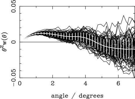
Figure 2: Lines as for Fig. 1, but now for the angular correlation function of 100 of the QPM CMASS mocks, binned into bins of width $\Delta\theta=0.16$ degrees.

To quantify the survey masks of both the CMASS and LOWZ samples, we used a catalogue of points chosen randomly to sample the survey regions, containing 20$\times$ as many points as the number of galaxies in each sample. Using the galaxy and random catalogues we have measured galaxy-galaxy (DD), galaxy-random (DR) and random-random (RR) pair-counts. The pair-counts were binned into $180\times 270$ bins with separation $\Delta r=1\,h^{-1}\,{\rm Mpc}$, $0<r<180\,h^{-1}\,{\rm Mpc}$ and linearly spaced in $0<\theta<9$ degrees for CMASS and $0<\theta<21$ degrees for LOWZ. We include pairs that are within the angular range considered, but have $r>180\,h^{-1}\,{\rm Mpc}$ in the final bin in $r$, so that our angular clustering can be measured as if there were no radial information. The range of angles considered is driven by calculating $w(\theta)$ for the pairs with the separations of interest, and so is different for LOWZ and CMASS samples. We have tried a number of resolutions for the angular pair count bins, and find that it does not significantly influence the results: for simplicity we downsample the angular pair counts by a factor of 5 for the results presented. As we only consider the monopole moment, we do not additionally bin in $\mu$, the cosine of the angle to the line-of-sight, although we would expect angular pair weighting to help improve the full 3D correlation function for all $\mu$ except $\mu=1$, which corresponds to $\theta=0$ and where the angular correlations are formally both zero. Using the Landy & Szalay (1993) estimator, we used these pair counts to measure the monopole moment of the correlation function for each mock catalogue. For a selection of the QPM CMASS mocks, these are plotted against their mean and variance in Fig. 1.

We wish to contrast the measured variance of the monopole correlation function with that obtained using angular pair upweighting as if we had a wider area of projected angular data. We have calculated the angular correlation function for mock $i$, $w_{i}(\theta)$, where we take the binned pair counts described above for $DD_{i}(\theta)$, $DR_{i}(\theta)$ and $RR_{i}(\theta)$ split by $\theta$ and use the Landy & Szalay (1993) estimator: the angular correlation functions for a selection of the QPM CMASS mocks are plotted in Fig. 2. In order to consider an angular clustering measurement made as if from a wider survey, we average angular pair-counts from the mock of interest and $N_{\rm proj}-1$ additional mocks, creating a lower-variance estimate of the $DD$ and $DR$ angular pair-counts:

$$\mkern 1.5mu\overline{\mkern-1.5muDD\mkern-1.5mu}\mkern 1.5mu_{i}(\theta)=\frac{1}{N_{\rm proj}}\sum_{i}^{i+N_{\rm proj}}DD_{i}(\theta),$$ (20)

and similarly for $\mkern 1.5mu\overline{\mkern-1.5muDR\mkern-1.5mu}\mkern 1.5mu_{i}$. We determine the ratios of counts in the low variance estimate to that from the individual mock, $\mkern 1.5mu\overline{\mkern-1.5muDD\mkern-1.5mu}\mkern 1.5mu_{i}(\theta)/DD_{i}(\theta)$ and $\mkern 1.5mu\overline{\mkern-1.5muDR\mkern-1.5mu}\mkern 1.5mu_{i}(\theta)/DR_{i}(\theta)$ in bins of width $\Delta\theta=0.16$ degrees. We use this ratio to weight the paircounts for each bin in $r$ and $\theta$, so our weighted estimate for $DD_{i}(r)$ is given by

$$\mkern 1.5mu\overline{\mkern-1.5muDD\mkern-1.5mu}\mkern 1.5mu_{i}(r)=\sum_{\theta}DD_{i}(r,\theta)\frac{\mkern 1.5mu\overline{\mkern-1.5muDD\mkern-1.5mu}\mkern 1.5mu_{i}(\theta)}{DD_{i}(\theta)}.$$ (21)

The monopole moment of the correlation function was then recalculated for each mock using $\mkern 1.5mu\overline{\mkern-1.5muDD\mkern-1.5mu}\mkern 1.5mu(r)$ and $\mkern 1.5mu\overline{\mkern-1.5muDR\mkern-1.5mu}\mkern 1.5mu(r)$. $RR(r)$ is unchanged as we use the same random catalogue for all mocks. The average weighted monopole matches the unweighted average with differences at the level expected from noise.

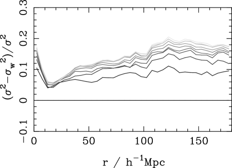
Figure 3: The fractional improvement in the variance for the CMASS DR12 NGP mocks assuming there is additional information on the angular correlation function corresponding to $N_{\rm proj}=2...10$ - i.e. between twice and 10$\times$ the area. $\sigma^{2}$ is the unweighted variance, and $\sigma_{w}^{2}$ is the variance after angular pair upweighting.

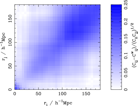
Figure 4: The fractional improvement in the correlation matrix for the CMASS DR12 NGP mocks assuming there is additional information on the angular correlation function corresponding to 10$\times$ the area. $C_{ij}$ is the element of the covariance matrix for $\xi_{0}$ between bins $i$ and $j$, and $C^{w}_{ij}$ is the covariance matrix element for the weighted correlation function.

Fig. 3 presents the fractional improvement in the variance obtained for the CMASS DR12 QPM mocks. We show the potential improvement as if we had between $2\times$ and $10\times$ the angular data with which to weight the 3D pair counts. Although unrealistic for BOSS, as the area covered by the NGP sample is already $\sim 7,000$ deg², this demonstrates the logarithmic improvement to the 3D clustering measurements possible with increasing amounts of angular data, matching the asymptotic behaviour of Eq. (18). Fig. 4 shows that the improvement in the covariance extends to the off-diagonal elements. For simplicity, we only show the improvement for the case of having $10\times$ the angular data with which to weight the 3D pair counts.

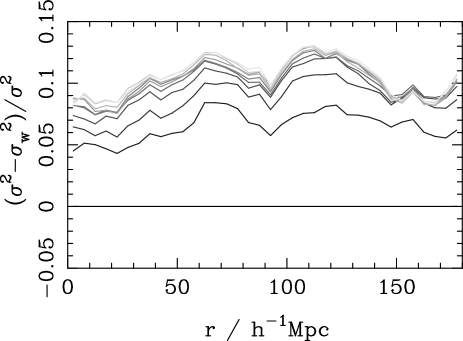
Figure 5: As Fig. 3, but now for the MD-Patchy LOWZ mocks.

The fractional improvement for the LOWZ DR12 MD-Patchy mocks is shown in Fig. 5. As in Fig. 3, we show the potential improvement as if we had between $2\times$ and $10\times$ the angular data with which to weight the 3D pair counts. The improvement for LOWZ is slightly worse than that for CMASS, asymptoting to a $\sim$10% improvement on BAO scales for large angular target areas.

5 Discussion

We have presented analytic and numerical arguments that angular-pair upweighting is an efficient method to enhance the 3D clustering measurements from spectroscopic surveys, when angular clustering data is available over a larger area than that observed spectroscopically. Results from both the analytic derivation and from mock catalogues show improvement in the error on the resulting 3D correlation function measurements. We have also shown that angular pair upweighting gives rise to unbiased clustering measurements.

In essence, the method works by exploiting the correlation between angular and 3D clustering: by dividing the spectroscopic pair counts by the angular pair counts, we remove this component of the noise, and we then multiply by an estimator with the same mean but lower noise to get back to an unbiased estimate of the 3D pair counts. In terms of radial and angular modes, we are using additional angular data to reduce the error on the contribution of these modes to the 3D clustering measurement.

Our analysis of mock catalogues shows a larger improvement than that in the toy analytic model, and the level of improvement is different for the LOWZ and CMASS samples: we expect this is because the monopole correlation function measurements are correlated for the mock data across different $r$, unlike the toy model. Angular projection acts as a smoothing of the monopole with an asymmetric kernel, and so the correlations between angular and 3D $\xi$ will be increased by coherence in the 3D $\xi$- i.e. the correlations in the clustering signal mimic slightly those of the angular projection. There will also be differences caused by changes in the relative importance of angular compared to radial clustering in the final measurement, due to survey geometry and redshift-space effects.

There are some caveats to the analysis presented: in particular, we have only tested the efficiency of pair upweighting using binned data. It would be possible to provide a weight for every galaxy pair using the actual separation (this was the procedure adopted in Bianchi & Percival 2017). However, using the binned counts is conservative and, given the number and size of the BOSS mocks used, using individual weights for each pair would have been prohibitively expensive.

It is not obvious how the proposed upweighting would affect clustering measurements post-reconstruction of the density field, which has become an essential part of BAO analyses. However, it should be possible to reap the benefits of pair upweighting, while including the information from reconstruction by following the recent work of Sanchez et al. (2016). This suggested that the combination of post-reconstruction and weighted pre-recon measurement could be performed after parameter measurement, while retaining the information from both. Practically, one would calculate upweighted pre-reconstruction clustering and non-weighted post-reconstruction clustering, and combine the measurements of cosmological parameters from both to form combined parameter measurements, allowing for correlations between measurements. The angular upweighting would reduce the correlation between pre- and post-reconstruction measurements, enhancing the combined signal.

For obvious reasons, the method works best where there is a strong correlation between 3D and angular clustering measurements, so it will provide a more significant improvement for thinner redshift shells. Thus, if photometric redshifts were provided for all target galaxies in the sample, including those with spectroscopic redshifts, these could be used to split the sample into thinner redshift shells before applying the angular upweighting. It would be possible to work with shells in photo-z, or using an interpolation scheme across redshift. This would enhance the efficiency of the weights.

As constructed, the method will work where the samples used are of the same underlying objects. Enhancing the 3D clustering using angular samples of a different population would be possible, but would come at the expense of having to model the cross-correlation. The method will help to improve both shot-noise and sample variance errors: for a narrow spectroscopic survey, upweighting using a wider angular sample of target galaxies will improve the sample variance error, while upweighting a sparse spectroscopic sample of a wide survey using a denser sample of angular pair counts over the same area would improve the shot noise.

References

- Alam et al. (2015) Alam S., et al., 2015, ApJS 219, 12
- Alam et al. (2016) Alam S., et al., 2016, arXiv:1607.03155
- Amir et al. (2016a) Amir S., et al., 2016a, arXiv:1611.00036
- Amir et al. (2016b) Amir S., et al., 2016b, arXiv:1611.00037
- Anderson et al. (2012) Anderson L., et al., 2012, MNRAS 427, 3435
- Bianchi & Percival (2017) Bianchi D., Percival W.J., 2017, arXiv:1703.02070
- Colless et al. (2003) Colless M., et al., 2003, [astro-ph/0306581]
- Dawson et al. (2013) Dawson K., et al., 2013, AJ, 145, 10
- Dawson et al. (2016) Dawson K., et al., 2016, AJ, 151, 44
- de la Torre et al. (2013) de la Torre S., et al., 2013, A&A, 557, A54
- de la Torre et al. (2016) de la Torre S., et al., 2016, arXiv:1612.05647
- Eisenstein et al. (2011) Eisenstein D.J., et al., 2011, AJ, 142, 72
- Guzzo et al. (2014) Guzzo L., et al., 2014, A&A, 566, 108
- Hawkins et al. (2003) Hawkins E., et al., 2003, MNRAS 346, 78
- Kitaura et al. (2016) Kitaura F.-S., et al., 2016, MNRAS, 456, 4156
- Landy & Szalay (1993) Landy S.D., Szalay A.S., 1993, ApJ 412, 64
- Laureijs (2011) Laureijs R., et al., 2011, arXiv:1110.3193
- Reid et al. (2016) Reid B., et al., 2016, MNRAS, 455, 1553
- Sanchez et al. (2016) Sanchez A., et al., 2017, MNRAS 464, 1493
- White et al. (2014) White M., Tinker J. L., McBride C. K., 2014, MNRAS, 437, 2594