Unbiased clustering estimation in the presence of missing observations

Abstract

In order to be efficient, spectroscopic galaxy redshift surveys do not obtain redshifts for all galaxies in the population targeted. The missing galaxies are often clustered, commonly leading to a lower proportion of successful observations in dense regions. One example is the close-pair issue for SDSS spectroscopic galaxy surveys, which have a deficit of pairs of observed galaxies with angular separation closer than the hardware limit on placing neighbouring fibres. Spatially clustered missing observations will exist in the next generations of surveys. Various schemes have previously been suggested to mitigate these effects, but none works for all situations. We argue that the solution is to link the missing galaxies to those observed with statistically equivalent clustering properties, and that the best way to do this is to rerun the targeting algorithm, varying the angular position of the observations. Provided that every pair has a non-zero probability of being observed in one realisation of the algorithm, then a pair-upweighting scheme linking targets to successful observations, can correct these issues. We present such a scheme, and demonstrate its validity using realisations of an idealised simple survey strategy.

1 Introduction

The clustering of galaxies observed in spectroscopic galaxy surveys provides a wealth of cosmological information. In order to extract this information we need to isolate and remove, or ignore, spatial galaxy-density fluctuations that arise from non-cosmological sources, including those that result from the way that observations are made. One potential source of these fluctuations is that of missing observations. For surveys using multi-object spectrographs to observe a target sample of galaxies selected from imaging surveys, it is usually prohibitively inefficient to observe and obtain spectra for 100% of the targets. The difficulty results from a combination of the anisotropic distribution of galaxies on the sky, a product of the very clustering to be measured, and the mechanical design of the instrument. Surveys therefore leave a small percentage of the target sample without spectra. The angular distribution of the missing galaxies depends on both the observing strategy (for example the number of times the survey covered a particular region), and the density of targets, and thus can produce a significant clustering signal.

For the updated Sloan telescope (Gunn et al., 2006) as used by the Baryon Oscillation Spectroscopic Survey (BOSS; Dawson et al., 2013) , the fibres cannot be placed closer than 62$\arcsec$ on the focal plane, and so if two targets are closer than this separation they cannot both be observed with a single pass of the instrument. Approximately $\sim 5$% of the targets in the final Data Release 12 (Alam et al., 2015) of BOSS were not observed as a consequence of fibre-collision (Reid et al., 2016). Because of the density-dependence of this sample, fibre-collisions have a strong effect on the small-scale clustering measurements, as described by Hahn et al. (2017), for example. The scales affected become even larger for deeper surveys such as the extended BOSS (Dawson et al., 2016) and the Dark Energy Spectroscopic Instrument (DESI; DESI Collaboration et al., 2016a, b).

To construct its main survey covering 14000 deg², DESI will make approximately 10,000 observations, taking 5000 spectra in each 7.5 deg² field-of-view. Although the average number of observations covering any patch in the survey is 5, the range is between 1 and 12. In regions of high target density, and for targets of low priority in the ranking of different target classes, there will be missing observations. Thus, unless corrected they have the potential to significantly distort measurements of cosmological clustering (Pinol et al., 2017; Burden et al., 2017).

In this paper, we consider the general problem of missing galaxies, in a way that is not tied to any survey, and present an algorithm for debiasing the measured correlation function. It works by determining a probability of selection for any pair and weighting by the inverse of this probability. This then provides an unbiased estimation of the correlation function, provided that any pair in the sample has a non-zero probability of being observed if it were moved to some location in the survey. The layout of our paper is as follows: in Sec. 2 we review the problem of missing observations; in Sec. 3 we present the derivation of our estimator; in Sec. 4 we define the selection algorithm that we use for testing; in Sec. 5 we discuss the behaviour of (a simplified version of) the estimator compared to that of the nearest neighbour assignment; in Sec. 6 we present the practical implementation of the estimator, which we compare to simulations in Sec. 7; we conclude summarising our results in Sec. 8.

2 Missing spectroscopic observations

We consider a general redshift survey, consisting of a set of targets with known angular positions, that we want to spectroscopically observe. If a randomly selected sample of targets does not have spectroscopic observations, then our estimate of the 3-dimensional overdensity at any location from the observed sample is unbiased, provided that the expected number of observations is reduced. e.g. suppose we define

$$\delta({\bf x})=\frac{\rho_{\rm all}({\bf x})}{\langle\rho_{\rm all}\rangle}-1,$$ (1)

then this $\delta$ is unaltered by the transformation $\rho_{\rm all}({\bf x})\to\alpha\rho_{\rm all}({\bf x})$ for any $\alpha<1$ that is spatially invariant.

We also do not need to worry about missing redshift measurements as a function of galaxy type. For example, suppose we target two classes of galaxies, each with a linear deterministic bias $\delta_{{\rm gal},A}=b_{A}\delta_{\rm mass}$, $\delta_{{\rm gal},B}=b_{B}\delta_{\rm mass}$, but only measure redshifts for galaxies in class $A$. Provided that we use $\langle\rho_{A}\rangle$ in the denominator when calculating $\delta$, then our estimate of $\delta$ only depends on the observed galaxies, and is unaffected by sample $B$.

Many surveys are not able to spectroscopically observe the full target sample, and make observations based on the angular target density. For example, the multi-object spectrograph on the Sloan telescope (Gunn et al., 2006) cannot simultaneously observe two targets closer than $62$ ″. This leads to a deficit of small angular separation pairs of galaxies, which is particularly severe for regions of the sky covered by only one pass of the instrument. In order to correct these effects, a number of approximate methods have been put forward (Anderson et al., 2012; Guo et al., 2012; Hahn et al., 2017). The standard approach adopted by the BOSS team has been to upweight by one the nearest target to each missing target (Anderson et al., 2012). To see how this works, consider pairs of galaxies as counted in standard correlation function measurements: the target nearest to that missed is statistically identical as there was a 50/50 chance as to which was observed, and it consequently has the same expected clustering properties. The upweight therefore approximately corrects the total pair count for missed pairs between the missed targets and other targets outside of the pair in question. The pair between the missed and nearest target is still excluded, and leads to a small-scale bias. Guo et al. (2012) suggested an algorithm that uses the regions of overlapping observations to understand those missed. However it does not works perfectly, because, as we discuss later, the observed pairs are not statistically identical to those missed. Reid et al. (2014) adopted a different approach where they assigned each missing galaxy the redshift of the nearest observed galaxy. This artificially creates small-separation pairs, but not necessarily with the correct distribution.

The situation is likely to be significantly worse for future surveys such as DESI (DESI Collaboration et al., 2016a, b), which will make observations using a grid of fibre feeds, with each fibre able to move independently, but only within its patrol radius. Even though the targets will be observed with multiple passes, the final set of spectroscopically observed targets will exhibit strong angular-density dependence. Two recent papers presented methods to combat the effect of missing galaxies due to the fibre assignment scheme of DESI. Pinol et al. (2017) showed that allowing for variations in coverage within the mask, commonly quantified by a random Poisson sampling and referred to as the “random catalogue” reduces this effect. They argue that the best way to completely mitigate the effect is to remove the angular modes from the analysis. Burden et al. (2017) advocate a similar approach, modifying the standard correlation function estimator in order to null angular modes, and demonstrated how this would work using mock data. Note that both of these approaches discard information rather than trying to understand and model the effects.

Given that we know the angular distribution of the targets, it has been suggested that, when calculating the 3-dimensional correlation function, we upweight each observed pair by the reciprocal of the fraction of observed pairs of targets with that angular separation (Hawkins et al., 2003). This correction does not work in general, because, again, it assumes that the radial properties of the unobserved pairs of targets are statistically equivalent to those of the observed pairs. Let us consider the example of the SDSS, given above. Here, missing close-pairs are more likely to be in triplets of targets than observed close-pairs: triples require three observations to fully observe, whereas doubles only require two, and the area covered by three observations is significantly smaller than that covered by two. Galaxies in triples of targets are more likely to be radially associated than galaxies in doubles, as they represent more unlikely chance alignments. The idea of upweighting of angular pairs is similar to the method put forward by Hahn et al. (2017), who probabilistically assigned galaxy redshifts to missing galaxies based on those observed. Both approaches use the observed galaxies to understand the unobserved ones, but the problem is also the same as that discussed above - that the missing pairs or galaxies and observed pairs or galaxies need to be carefully matched: the matching between observed and unobserved pairs is at the heart of any scheme to correct for missing observations.

3 The new algorithm

In this section we present a new method to match observed and unobserved pairs. As we consider pairs of galaxies, it is easiest to consider this in the context of the measurement of the correlation function. We argue that this matching between observed and unobserved targets is simpler if we work with pairs rather than galaxies, as the selection algorithm can act over large scales, meaning it is difficult to select galaxies in the observed sample that match those that are missing. Because the calculation of the correlation function only depends on the numbers of pairs, by matching pairs we can be sure that we are including all of the necessary information.

One final assumption we make is that all pairs have non-zero probability that they could be observed were we allowed the freedom to move them to any spatial location covered by the observations. So there are no pairs of targets that represent objects that could never be observed. Both the SDSS BOSS and eBOSS surveys and DESI match this requirement.

3.1 The effect of adding and removing galaxies

We consider a given realisation of some anisotropically clustered random field, traced by a set of particles. We can measure the number of pairs in a given separation bin $\vec{s}\pm\Delta\vec{s}/2$, which we refer to as $DD(\vec{s})$. Suppose that we choose one galaxy and remove from our counts all the pairs formed by this galaxy, but we count twice the pairs formed by another galaxy. Plus we include in the counts the single pair formed by these two galaxies. We then have a new value $DD_{1}(\vec{s})\neq DD(\vec{s})$. Similarly, we can interchange the two selected galaxies and get $DD_{2}(\vec{s})\neq DD_{1}(\vec{s})\neq DD(\vec{s})$. Trivially, $[DD_{2}(\vec{s})+DD_{1}(\vec{s})]/2=DD(\vec{s})$, or, in other words, the mean of the two new counts corresponds to the original one. If realisation 1 and 2 are statistically equivalent, i.e. the probability of having 1 or 2 is apriori identical, their mean corresponds to the expected value of an unbiased estimator for $DD(\vec{s})$. This simple argument can be invoked to justify standard countermeasures against the fibre-collision issue, such as the nearest neighbour upweighting (e.g. Anderson et al., 2012). We will show that this class of weighting schemes can be seen as approximations, formally not unbiased, of a more rigorous and general description of the problem.

3.2 Unbiased estimator

The evaluation of two-point statistics in a galaxy survey is based on pair counts at different separations $\vec{s}$, e.g. if we want to measure the correlation function a standard approach is to use the following estimator (Landy & Szalay, 1993):

$$\hat{\xi}(\vec{s})=\frac{DD(\vec{s})}{RR(\vec{s})}-2\frac{DR({\vec{s}})}{RR(\vec{s})}+1\ ,$$ (2)

where $DD$ is the number of data (i.e. galaxy) pairs, $RR$ is the number of pairs in a random catalogue covering the same volume of the survey and $DR$ is the number of data-random pairs.

Suppose we have an algorithm to extract a subset of galaxies from the full sample according to some arbitrary selection rule. Since this selection algorithm is completely free, in general, the pair counts $DD(\vec{s})$ in the new sample and those from the original parent sample $DD_{p}(\vec{s})$ will differ, in both shape and amplitude (and similarly for $DR$). Suppose that, as in any realistic scenario, the algorithm is stochastic, i.e. for a given galaxy sample there are many possible outcome subsets, corresponding to different random seeds. The quantity of interest is then the expectation value of $DD$ and $DR$ (obviously $RR=RR_{p}$ remains unchanged). Still, for a generic algorithm $\langle DD\rangle\neq DD_{p}$, and similarly for $DR$.

If we denote with $p_{i}$ the probability of the $i$-th galaxy of being selected, the probability that the pair formed by the $m$-th and $n$-th galaxies contributes to the counts is

$$p_{mn}=p_{m}p_{n}(1+c_{mn})\ ,$$ (3)

where

$$c_{mn}\equiv\ \frac{p_{mn}}{p_{m}p_{n}}-1$$ (4)

is the selection correlation associated to that specific pair.

Each pair carries two fundamental pieces of information: the separation $\vec{x}_{m}-\vec{x}_{n}$ and the selection probability $p_{mn}$. As we will see, in general the latter cannot be reduced to the former. It is natural to use this probability to correct the galaxy pair counts. Specifically, we define the statistical weight of each pair as

$$w_{mn}\equiv\frac{1}{p_{mn}}\ .$$ (5)

At any separation the pair count is then given by

$$DD(\vec{s})=\sum_{\vec{x}_{m}-\vec{x}_{n}\approx\vec{s}}w_{mn}\ ,$$ (6)

where the symbol “$\approx$” means that the sum is performed over pairs whose separation falls in a specific $\vec{s}$ bin. Obviously only pairs selected by the algorithm are considered.

By construction, if each pair has non-zero probability of being selected, the expectation value of the so obtained $DD$ is unbiased, i.e. $\langle DD\rangle=DD_{p}$. This can be understood by observing that, with the pairwise-inverse-probability (PIP) weighting scheme just introduced, if we sum over $N$ realisations, statistically, each pair appears $N$ times and, as a consequence, each pair contributes a term $N/N=1$ to the average pair counts. On scales where at least one of the pairs has null selection probability, the PIP scheme is potentially biased, reflecting the fact that the information on that pair is completely lost. Trivially, when a pure fibre-collision issue is considered, no pair below some minimum-fibre-separation scale $r_{f}$ can be observed and the estimator is not only biased but completely uninformative on such scales.

Inspired by Eq. (3), we can rearrange the pair weights as follows

$$w_{mn}=w_{m}\ w_{n}\ w^{(c)}_{mn}\ ,$$ (7)

where we defined $w_{i}\equiv 1/p_{i}$ and $w^{(c)}_{mn}\equiv 1/(1+c_{mn})$. This makes clear that, if the selection correlation is negligible, pair weighting can be reduced to galaxy weighting, i.e. $w_{mn}=w_{m}w_{n}$.

As regards $DR$ counts, galaxy weighting is always sufficient, since the selection algorithm does not apply to the random sample and, as a consequence, the selection probability of a galaxy-random pair always reduces to the individual probability of the galaxy.

Note that all the above considerations do not necessarily have be related to a fibre-collision issue. The description is formally valid for any scenario in which a subset of particles is extracted from a larger sample with known selection probability.

4 Selection algorithm and correlation length

In the following we focus more explicitly on a fibre-collision-like problem, which means we consider only selection criteria based on the angular position of the galaxies. For simplicity, we assume the plane parallel approximation, i.e. the angular separation of pairs corresponds to the perpendicular-to-the-line-of-sight separation $s_{\perp}$.

In order to help to demonstrate the more general idea, we define a specific selection algorithm, which we use for testing. We explicitly discuss throughout the paper which of our results depends on this particular choice. The algorithm we adopt is meant to maximise the randomness of the selection criteria in the presence of fibre collisions, which is why hereafter we refer to it as the maximum randomness (MR) algorithm. It can be summarised as follows: we randomly pick a pair among those with angular separation smaller than $r_{f}$ and randomly discard one of the two galaxies; we iterate the procedure until there are no more pairs with angular separation smaller than $r_{f}$.

Given the geometry of problem we are studying, it is useful to introduce the concept of angular friend-of-friend (AFOF) halo, obtained by restricting the standard friend-of-friend definition (e.g. Davis et al., 1985) to the angular separation only, i.e. ignoring the line-of-sight coordinates of the galaxies, with linking length given by the minimum-fibre-separation scale $r_{f}$.

With the MR algorithm the selection probability of individual galaxies is independent on scales larger than $r_{c}$, this latter being the largest separation between two galaxies belonging to the same AFOF halo, or, roughly speaking, the size of the largest AFOF halo in the sample. In other words, whether a galaxy is selected or not in general depends on all the other galaxies belonging to the same halo, but not on the galaxies outside that specific halo. For more complex algorithms we can think of generalising $r_{c}$ as the correlation length above which the selection correlation introduced in Eq. (4) becomes negligible. In any case, for $s_{\perp}>r_{c}$ the pairwise probability reduces to the product of individual probabilities, and our unbiased estimator, Eq. 6, can be expressed in terms of galaxy weights,

$$DD(\vec{s})=\sum_{\vec{x}_{m}-\vec{x}_{n}\approx\vec{s}}w_{i}w_{j}\ .$$ (8)

These individual-inverse-probability (IIP) weights can be evaluated analytically if the selection algorithm is simple enough (see Sec. 5.1) or, more realistically, estimated numerically. Note that $r_{c}$ is a well-defined number that can be measured from the sample under examination. For $s_{\perp}<r_{c}$ we need to enforce pair weighting as specified in Eq. (6). Unfortunately, $r_{c}$ grows fast with the galaxy number density and the collision scale $r_{f}$, thus making pair weighting in general preferable. Analogously to the individual one, the pair probability can be in principle computed analytically or, more pragmatically, evaluated numerically, with the obvious complication of having to deal with $N^{2}$ objects rather than just $N$.

5 Galaxy weighting

In this section we compare two examples of individual-galaxy weighting schemes, namely the IIP approach, defined by Eq. (8), and the well know nearest neighbour (NN) correction, which consists of assigning the weight of the missing galaxy to its nearest (in terms of angular position) observed companion. Two more galaxy-weight prescriptions, with performances comparable to those of the NN assignment, are considered in App. A. As discussed above, weighting individual galaxies is not the most general possible approach to the problem of missing observation, since it does not account for selection correlation. Dealing with this issue actually requires a pair-weighting approach, which we present in Sec. 6. It is nonetheless instructive to see how, even in this simplified scenario, a probability-oriented reasoning is convenient with respect to the more standard idea of moving weights from the missing to the observed galaxies, which is behind the NN correction.

5.1 Case study

Here we discuss a simple example of a small structure of target galaxies, which hopefully will help to clarify a few basic concepts. We consider a single AFOF structure, sketched in Fig. 1.

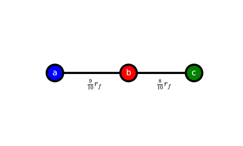
Figure 1: Partially collided triplet formed by the collided pairs $\{a,b\}$ and $\{b,c\}$. The line of sight is perpendicular to the plane of the figure. The intra-particle separations are expressed in units of the collision length $r_{f}$, which in a pure fibre-collision problem is just the size of the fibre. Only collided pairs, i.e. those with separations smaller than $r_{f}$ are connected by solid lines.

We define the triplet $\{a,b,c\}$ as a partially collided structure, formed by two collided structures, the pairs $\{a,b\}$ and $\{b,c\}$. We consider pairs with different separation just to avoid degeneracy when applying the NN scheme. All the calculations in this section refer to the MR algorithm defined in Sec. 4. When applied to the AFOF halo in the figure, the NN scheme yields

$$S^{(NN)}=\begin{bmatrix}1&0&2\\ 0&3&0\\ 0&0&3\\ 3&0&0\end{bmatrix}\quad,\quad P^{(NN)}=\begin{bmatrix}1/2\\ 1/4\\ 1/8\\ 1/8\end{bmatrix}\ ,$$ (9)

where each row of the matrix $S^{(NN)}$ represents one of the possible set of weights $\{w_{a},w_{b},w_{c}\}$ associated to the galaxy triplet. The array $P^{(NN)}$ represents the correspondent probability, which is evaluated analytically. Trivially, only selected galaxies can have non-zero weight. The number of objects is conserved, i.e. the sum of the elements of a row is always 3. The sum of the elements of the columns, weighted by the correspondent probability, is $\{11/8,3/4,7/8\}$. This means that the estimator is biased, since, in order to play the game described in Sec. 3 we need this sum to be $\{1,1,1\}$. More explicitly, if the AFOF halo under examination is the only collided structure in the universe, then the selection probability of the cross pairs formed by a galaxy belonging to the halo with all the external ones is exactly given by the individual probability of the former. As a consequence, when the weighted sum is $\{1,1,1\}$ the cross-pair count is formally unbiased, in the sense that its mean is exactly what we would have without any selection process (i.e. fibre collision). For this specific example, it means $\langle DD\rangle=DD_{p}$ on scales $s_{\perp}>17/10\ r_{f}$, which is the size of the largest pair in the halo, namely pair $\{a,c\}$. This reasoning can easily be extended to the general scenario in which there are several AFOF halos in the sample, since the resulting cross probabilities are disjoint by construction.

With the IIP scheme we instead obtain

$$S^{(IIP)}=\begin{bmatrix}8/5&0&8/5\\ 0&4&0\\ 0&0&8/5\\ 8/5&0&0\end{bmatrix}\quad,\quad P^{(IIP)}=\begin{bmatrix}1/2\\ 1/4\\ 1/8\\ 1/8\end{bmatrix}\ .$$ (10)

In this case each galaxy is weighted by its inverse probability of being selected by the algorithm. At variance with $S^{(NN)}$, for $S^{(IIP)}$ the number of objects is not conserved, but the estimator is unbiased, since the weighted sum of the elements of each column is $\{1,1,1\}$ by construction. The fact that the galaxy number is not conserved suggests that the higher accuracy of this estimator comes at the cost of less precision (i.e. no bias but larger variance). We show in Sec. 6.2 how to circumvent this issue.

One interesting question is whether the pair counts are correct inside the structure under consideration. Obviously, this cannot be the case for pairs with angular separation $s_{\perp}<r_{f}$ since none of these pairs can be observed by definition, but it could still be true for the pair $\{a,c\}$. Indeed, for the NN scheme, the pair $\{a,c\}$ is correctly weighted, in the sense that, when summing over $N$ different realisations, statistically, this pair is counted $N$ times, i.e one time in average: $\sum_{i}S^{(NN)}_{i1}S^{(NN)}_{i3}P^{(NN)}_{i}=1$. One might wonder if this is a general property of the NN assignment. It is then useful to consider a further example, which shows that this is not the case.

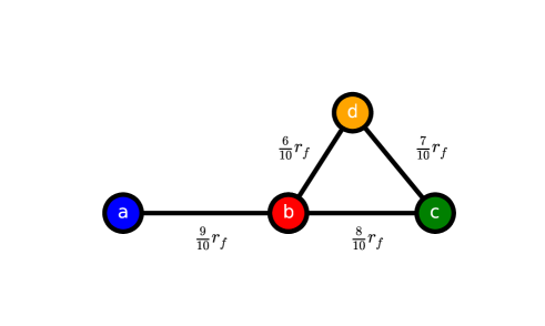
Figure 2: Partially collided structure formed by the collided pair $\{a,b\}$ and the collided triplet $\{b,c,d\}$. Same notation as in Fig. 1.

We repeat our calculations for a new AFOF structure, obtained by adding a forth galaxy $d$ to the previously discussed triplet, as sketched in Fig. 2. We get

$$S^{(NN)}=\begin{bmatrix}1&0&3&0\\ 1&0&0&3\\ 0&4&0&0\\ 0&0&4&0\\ 0&0&0&4\\ 4&0&0&0\end{bmatrix}\quad,\quad P^{(NN)}=\begin{bmatrix}5/16\\ 5/16\\ 1/6\\ 7/96\\ 7/96\\ 1/16\end{bmatrix}\ ;$$ (11)

$$S^{(IIP)}=\begin{bmatrix}16/11&0&96/37&0\\ 16/11&0&0&96/37\\ 0&6&0&0\\ 0&0&96/37&0\\ 0&0&0&96/37\\ 16/11&0&0&0\end{bmatrix}\quad,\quad P^{(IIP)}=\begin{bmatrix}5/16\\ 5/16\\ 1/6\\ 7/96\\ 7/96\\ 1/16\end{bmatrix}\ .$$ (12)

Clearly, the complexity of the analytical calculations grows fast with the number of particles involved. As anticipated, the number of pairs with $s_{\perp}>r_{f}$ inside the AFOF halo is in general not conserved (for $s_{\perp}<r_{f}$ this number has to be zero by construction). For instance, the average counting of pair $\{a,c\}$ is $15/16$ and $480/407$ for NN and IIP, respectively, meaning that neither of the two corrections is unbiased for $r_{f}<s_{\perp}<r_{c}$. At least for IIP, this is not a surprise, since on scales smaller than $r_{c}$, by definition, the selection correlation cannot be neglected when evaluating the pairwise probability.

Finally, the comparison between the two AFOF structures, Figs. 1 and 2, provides us with the proof that the selection probability cannot be deduced by the separation only: despite the separation between galaxy $a$ and $c$ being fixed, the selection probability of pair $\{a,c\}$ drops from $1/2$ to $5/16$ when galaxy $d$ is added.

5.2 Range of validity

In order to summarise the properties of the above estimators, it is useful to divide the $s_{\parallel}$-$s_{\perp}$ plane into three regions. These regions are defined by the two characteristic scales already introduced, $r_{f}$ and $r_{c}$. The former represents the minimum allowed angular separation between galaxies, e.g. the size of the fibre. The latter is the largest angular separation between two galaxies belonging to the same AFOF structure, where the linking length is $r_{f}$ (or, in a more general scenario, just a selection-correlation length). Both the estimators discussed above are potentially biased for $r_{f}<s_{\perp}<r_{c}$ and completely uninformative for $s_{\perp}<r_{f}$. The IIP estimator is rigorously unbiased in the plane $s_{\perp}>r_{c}$, whereas the NN assignment is not, unless all the AFOF halos are purely collided structures (i.e. not partially collided). In other words, if we pick a single random galaxy from each AFOF halo, these latter estimator is unbiased as well. In general, we can think of the NN and similar schemes, such as those discussed in App. A, or found in the literature, e.g. local density weighting (e.g. Pezzotta et al., 2016), as an approximation of the IIP scheme. How reliable these approximations are strongly depends on the characteristics of the galaxy survey, such as the fraction of collided pairs among the total number of partially-collided structures.

6 Pair weighting

So far we have shown that it is convenient to: (i) see weights as inverse probabilities; (ii) weight pairs rather than individual galaxies. In the following we show that this is not only convenient but also feasible, by providing a practical implementation of the PIP method, which includes important considerations about how to reduce the variance of our estimator. But first we focus on how to extend our clustering estimate down to arbitrary small separations.

6.1 Including small scales

As we have already discussed, the PIP weighting scheme is unbiased by construction on scales larger than $r_{f}$, for a pure fibre collision issue, where $r_{f}$ is the diameter of the fibre. For a completely general selection algorithm, PIP is unbiased on all the scales for which no pair has null selection probability. This suggests that an all-scale unbiased estimator of the two-point functions can be obtained by removing the $r_{f}$ constraint in small random regions of the survey. Practically, this can be obtained by observing more than once a subset, not necessarily connected, of the whole sample. Overlap regions in the observing strategy are indeed quite common in modern surveys. It is important to emphasise that a 100% coverage of this subset is not necessarily needed. Indeed, in order to break the $r_{f}$ constraint it suffices to observe twice a region randomly picked from the total survey area, regardless of the fact that we might still miss objects in such a region (but, obviously, the more the galaxies we observe, the more the information that we can extract).

6.2 Minimising the variance: angular upweighting

So far we have focused on the bias of the estimator. We now move our attention to the issue of minimising its variance. To this purpose, we note that there is further information available, which we have not used yet, namely the knowledge of the angular correlation function of the full parent sample. In a companion paper (Percival & Bianchi, 2017) we explicitly discuss how, under quite general assumptions, this information can be used to build minimum variance estimators. Specifically we show that applying an angular upweighting (AUW, e.g. Hawkins et al., 2003) correction to an unbiased estimator whose variance is nearly Poissonian, has the beneficial effect of minimising the variance of this latter while leaving its expectation value unchanged. We therefore define our final weighting scheme as

$$DD(\vec{s})=\sum_{\vec{x}_{m}-\vec{x}_{n}\approx\vec{s}}w_{mn}\frac{DD^{(p)}_{a}(s_{\perp})}{DD_{a}(s_{\perp})}\ ,$$ (13)

where $DD^{(p)}_{a}$ and $DD_{a}$ represent the angular pair counts of the parent and the observed sample, respectively, whereas $w_{mn}$ is the PIP factor previously introduced. Note that $DD_{a}$ is, in turn, computed via the same $w_{mn}$ weights. Analoguosly, for the cross count we define $DR=\sum w_{m}\ DR^{(p)}_{a}/DR_{a}$, where the PIP weight of the galaxy-random pair is fully characterised by the individual weight $w_{m}$ of the galaxy.

Note also that it may be possible to further reduce the variance by a sensible selection of target galaxies. Any population or sub-population where only a small fraction of pairs will be recovered will in general, when added to the full sample, increase the shot noise of the population as a whole as we will be upweighting a small number of pairs. By judging the relative shot noise of sub-populations, if they can be selected from the full target sample, we should be able to judge whether or not they are worth including in the analysis.

6.3 Practical implementation: bitwise weights

In general, finding an efficient PIP-weighting implementation is not a trivial task. First, although in principle it is formally possible to compute analytically the weight associated to each pair, in practice this requires us to identify all the classes of collided structures in the sample and solve explicitly for the probability of the pairs there within, similarly to the calculation presented for the two simple examples discussed in Sec. 5.1. Even in the presence of a very simple selection algorithm, a dense sample is enough to make the analytical calculations unfeasible, due the complexity of the resulting collided structures. This problem can be circumvented by estimating the probabilities numerically by randomly repeating the selection process several times and estimating the probability of a given pair from the frequency with which it is chosen. Second, future galaxy surveys will collect spectra from $N_{gal}\sim 10^{7}$ galaxies, which implies $N_{gal}^{2}\sim 10^{14}$ pair weights with a consequent storage issue (which becomes catastrophic for higher order statistics).

We therefore introduce an effective scheme that retains all of the information about the pair weighting resulting from repeated applications of the targeting algorithm, but scales as $N_{gal}$. The selection probability of any galaxy can be recorded using $N_{n}/N_{bits}$, where $N_{n}$ is the number of times the $n$-th galaxy has been chosen and $N_{bits}$ is the total number of realisations of the selection process. In other words, $N_{n}=\sum_{i=1}^{N_{bits}}s^{(n)}_{i}$, where ${\bf s}^{(n)}$ is a logical array of length $N_{bits}$ whose $i$-th element is equal to 1 or 0 according to whether the galaxy has been selected or not in the $i$-th realisation, e.g. ${\bf s}^{(n)}=\{1,0,1,\dots,0,0,1\}$. From these data, the probability associated to a given pair is $N_{nm}/N_{bits}$, with $N_{nm}=\sum_{i=1}^{N_{bits}}s^{(n)}_{i}s^{(m)}_{i}$. As any logical array ${\bf s}$ can be seen as the binary representation of an integer number, the concept of weighting individual objects rather than pairs can be formally saved using such an approach.

In this case, we should drop the usual idea that the pair weight should be obtained as the product of galaxy weights, $w_{mn}=w_{m}w_{n}$. Indeed, by defining $w^{(b)}$ ($b$ stands for bitwise) as the integer number corresponding to ${\bf s}$, we have

$$w_{mn}=\frac{N_{bits}}{\operatorname{popcnt}\left[w^{(b)}_{m}\ \operatorname{and}\ w^{(b)}_{n}\right]}$$ (14)

where $\operatorname{and}$ and $\operatorname{popcnt}$ are standard (and extremely fast) bitwise operators. The former multiplies two integers bit by bit, whereas the latter is a population-count operator, which takes an integer and returns the sums of its bits. Since current computers rely on 32 or 64 bit architectures, for realistic choices of $N_{bits}$, large enough for an accurate sampling of the selection probability, e.g. $N_{bits}\sim 10^{3}$, we need to split $w^{(b)}$ into $\sim 10$ sub-weights. This obviously makes the evaluation of $w_{mn}$ slower but still tractable. Finally it is important to note that Eq. (14) can be trivially extended to any higher order statistics just by iterating the $\operatorname{and}$ operator.

7 Comparison to simulations

observing strategy	$\bar{f}_{s}$	$\bar{f}_{d}$	$f_{c}$	$f_{u}$	$f_{px}$	$f_{p1}$
OS1	$0.56$	$0.44$	$0.75$	$0.25$	$0.75$	$0.25$
OS2	$0.84$	$0.16$	$0.75$	$0.25$	$0.49$	$0.51$
OS2sub	$0.63$	$0.37$	$0.75$	$0.25$	$0.75$	$0.25$
OSmulti	$0.66$	$0.34$	$0.75$	$0.25$	$0.75$	$0.25$

Table 1: From left to right: average fraction of selected galaxies; average fraction of discarded galaxies; fraction of collided galaxies; fraction of uncollided galaxies; fraction of galaxies with selection probability $0<p<1$; fraction of galaxies with selection probability $p=1$. Each row corresponds to one of the four different observing strategies discussed in Sec. 7.

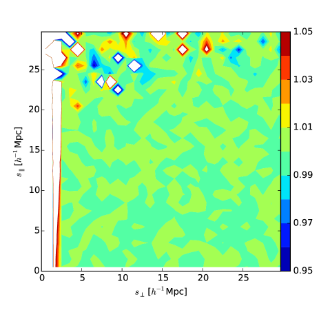
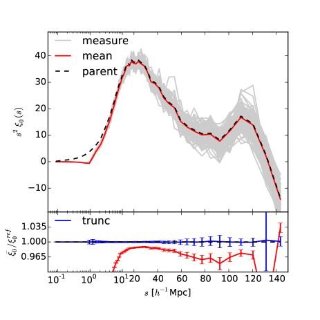
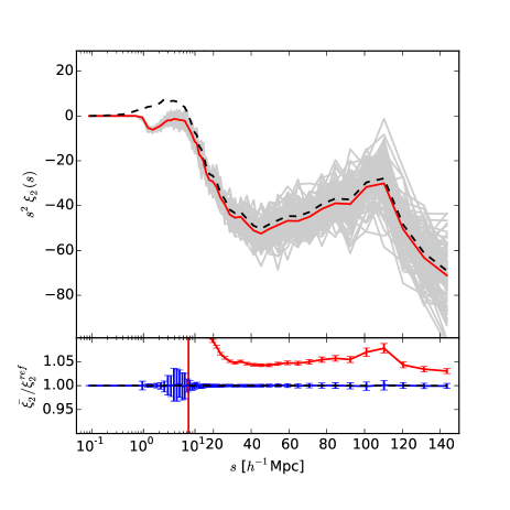
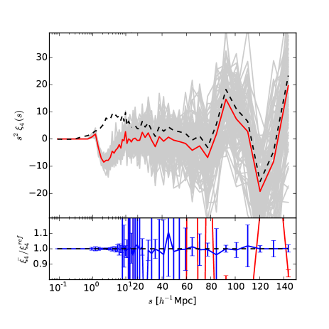
Figure 3: Performance of the PIP weighting scheme for the observing strategy OS1. Top left: ratio between the 2D correlation function $\xi(s_{\perp},s_{\parallel})$ obtained by averaging over 992 realisations of the selection process and the reference value measured from the full parent sample. Top right: an assortment of measurements of the Legendre monopole $\xi_{0}(s)$ extracted from the 992 realisations, solid grey, and the total mean, solid red, compared to the reference value, black dashed. In the bottom frame we show the ratio between the mean and the reference value, solid red, together with the ratio between the mean and the value recovered from the parent sample when the $s_{\perp}<r_{f}=1\,h^{-1}\,{\rm Mpc}$ stripe is excluded, blue solid, with error bars of the mean. In order to show both the large- and small-scale clustering features at once, we adopt a logarithmic scale for the abscissa for $s_{\perp}<15\,h^{-1}\,{\rm Mpc}$ and linear elsewhere. Bottom left and bottom right: same as top right but for the quadrupole $\xi_{2}(s)$ and the hexadecapole $\xi_{4}(s)$, respectively.

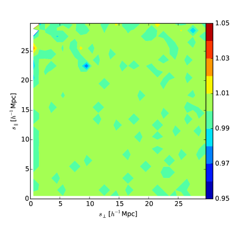
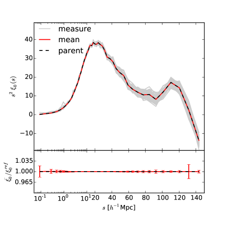
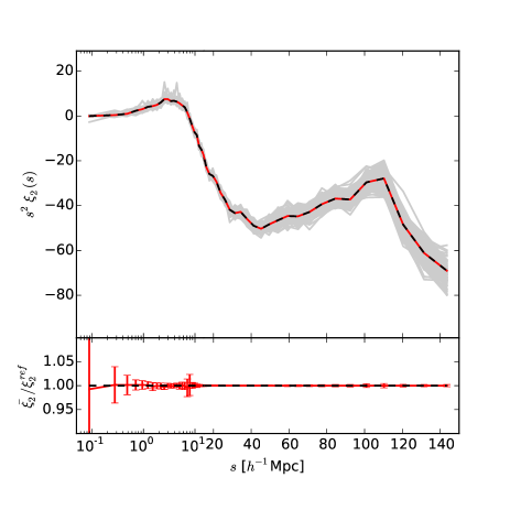
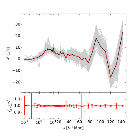
Figure 4: Same as Fig. 3 but for observing strategy OS2.

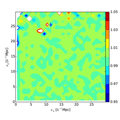
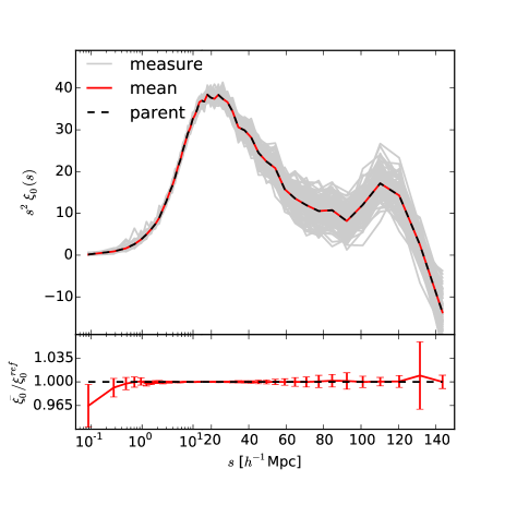
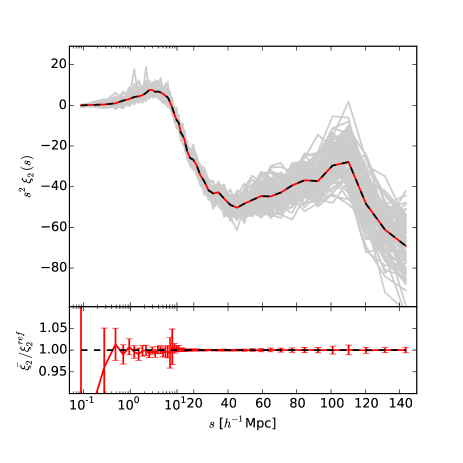
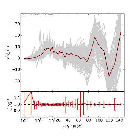
Figure 5: Same as Fig. 3 but for observing strategy OS2sub.

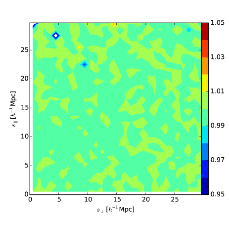
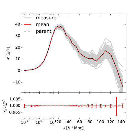
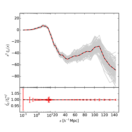
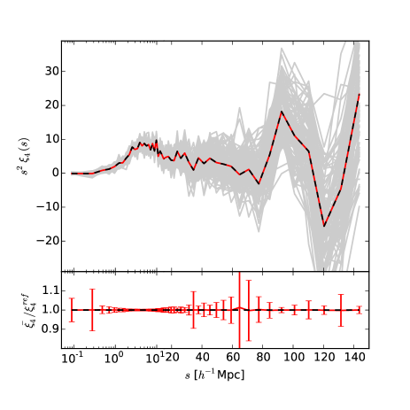
Figure 6: Same as Fig. 3 but for observing strategy OSmulti.

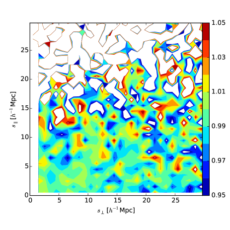
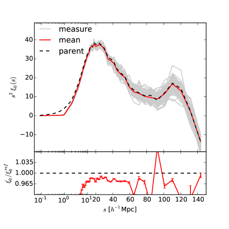
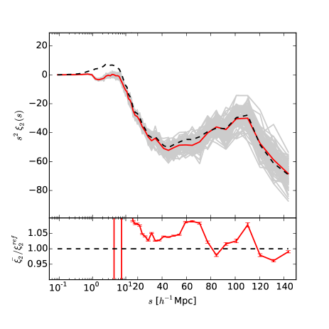
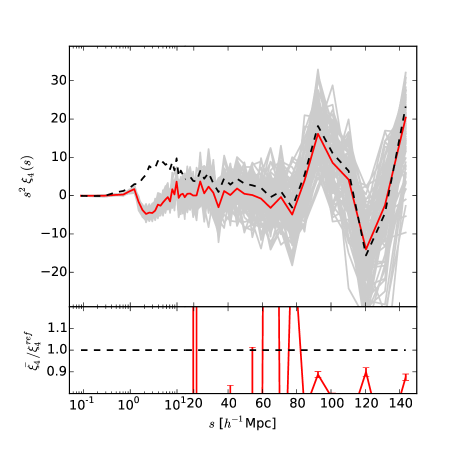
Figure 7: Same as Fig. 6 but with NN assignment instead of PIP correction.

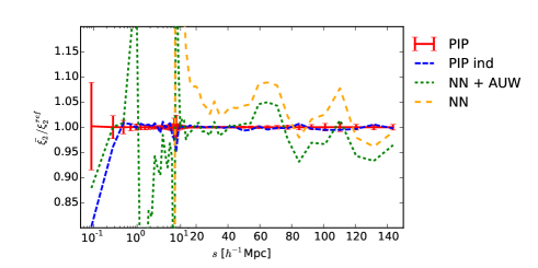
Figure 8: Comparison of the accuracy of the quadrupole measured via PIP, PIP derived from and independent set of realisations of the selection process, NN, NN plus AUW, as labeled in the figure. Only OSmulti is considered.

One of the properties that makes the PIP description preferable with respect to more standard approaches is that it can be coupled to any selection algorithm and parent sample, regardless, e.g., of the selection correlation length. Therefore, when testing the PIP weights against simulations, we do not try to mimic any specific survey but rather provide a general proof of concept for the method. We use the data from the MultiDark MDR1 run (Prada et al., 2012), which adopts WMAP cosmology, $\{\Omega_{m},\Omega_{\Lambda},\Omega_{b},\sigma_{8},n_{s}\}=\{0.27,0.73,0.047,0.82,0.95\}$, to describe the evolution of $2048^{3}$ particles over a ${(1000\,h^{-1}\,{\rm Mpc})}^{3}$ cubical box. For our analysis we apply a $0.005\%$ dilution factor to the snapshot at redshift $z=0.5$. The resulting catalogue consists of $\sim 4.3\times 10^{5}$ dark matter particles, corresponding to a $\sim 4.3\times 10^{-4}\text{h}^{3}\text{Mpc}^{-3}$ number density, which is compatible with the actual number density of targets in a modern galaxy survey. In the following we sometimes refer to these particles as galaxies and to this catalogue as the parent sample. All the collided catalogues we consider are obtained by applying, at least once, the MR algorithm to the parent sample, in redshift space (we assume plane-parallel approximation), with $r_{f}=1\,h^{-1}\,{\rm Mpc}$.

We first evaluate the effectiveness of our correction after a single pass of the MR selection algorithm. By repeating this observing strategy, which we refer to as OS1, for different random seeds of the algorithm, we have created 992 independent realisations all extracted from the same parent sample (we discuss later the impact of keeping the parent sample fixed).

The average fraction of galaxies that remain after this pass is $\bar{f}_{s}\sim 0.56$. Only about half of them, i.e. one fourth of the total, can be classified as uncollided because we have deliberately set an aggressive value of $r_{f}$ in order to produce a significant effect. Each galaxy belonging to this class has no other galaxies at separation smaller than $r_{f}$, or, in other words, its probability of being selected after a single pass is one.

In addition to $\bar{f}_{s}$, in Table 1 we report the fraction of discarded, collided and uncollided galaxies, for which we adopt the subscripts $d$, $c$ and $u$, respectively. Different observing strategy are considered. We also report $f_{px}$ and $f_{p1}$, which represent the fraction of galaxies for which the probability of being selected is $0<p<1$ and $p=1$, respectively. By construction none of the galaxies has selection probability $p=0$. When OS1 is adopted, trivially $f_{c}=f_{px}$ and $f_{u}=f_{p1}$.

In the top left panel of Fig 3, we show the ratio $\bar{\xi}(s_{\perp},s_{\parallel})/\xi_{p}(s_{\perp},s_{\parallel})$ between the average 2D correlation function measured via the PIP correction from the 992 realisations and that of the parent sample. PIP weights are inferred from the same 992 realisations, as described in Sec. 6.3, which means that we adopt $N_{bits}=992=31\times 32$ bits. This choice is arbitrary, based on our checks, it seem likely that a significantly smaller number, e.g. five times smaller, could be adopted for this quantity, if needed. However, the minimum acceptable $N_{bits}$ should be determined according to the specifics of survey and selection algorithm, which clearly goes beyond the purpose of this work. For the 2D correlation we focus on relatively small scales in order to emphasise the $s_{\perp}<r_{f}$ stripe and because on larger scales, the behaviour of $\xi$ becomes noisy due to the small bin sizes. See App. B for details on how we measure the different statistics and the corresponding binning. As expected, the PIP correction provides an unbiased estimate on all scales $s_{\perp}>r_{f}$. In the top right panel we explicitly show the Legendre monopole $\xi_{0}(s)$ measured from the various realisations, grey solid, together with the mean $\bar{\xi}_{0}$, red solid, and that measured from the parent sample $\xi_{0}^{ref}$, black dashed. At the bottom of the same panel we report the ratio $\bar{\xi}_{0}/\xi_{0}^{ref}$ with corresponding error bars of the mean. Similarly, in the bottom panels we show the behaviour of the Legendre quadrupole $\xi_{2}(s)$ and hexadecapole $\xi_{4}(s)$. In order to properly visualise the impact of fibre collisions on all the scale of interest, for these plots we adopt a logarithmic scale for $s<15\,h^{-1}\,{\rm Mpc}$, which becomes linear at larger separations. All of the multipoles are clearly affected by systematic bias, which grows with the order of the multipole. This is not surprising at all since the evaluation of the multipoles requires $\xi(s,\mu)$ to be integrated over the range $0\leq\mu\leq 1$, where $s=\sqrt{s_{\perp}^{2}+s_{\parallel}^{2}}$ and $\mu=s_{\parallel}/s$. As a consequence the $s_{\perp}<r_{f}$ stripe, in which the measurements are unavoidably uninformative when OS1 is adopted, affects the accuracy of our estimates on all scales. In practice, this problem can be easily circumvented just by excluding such band from the integration, i.e. using truncated multipoles (see e.g. Reid et al., 2014; Mohammad et al., 2016). In order to prove this, in addition to the ratio $\bar{\xi}_{n}/\xi_{n}^{ref}$, we also report $\bar{\xi}_{n}/\xi_{n}^{trunc}$, blue solid, where $\xi_{n}^{trunc}$ are the multipoles recovered from the parent sample using only the relevant scales, $s_{\perp}>r_{f}$. Clearly the systematic effect is removed.

Next, we consider the possibility of running a second pass of observations, in which the MR algorithm is applied to the galaxies discarded after the first pass (observing strategy OS2). With this new strategy we obviously see a large improvement in the estimate of the 2pt statistics, Fig. 4. Specifically, after PIP correction, $\xi(s_{\perp},s_{\parallel})$ is now unbiased on all scales (top left panel), as expected, i.e. we now have pairs and can estimate $\xi$ for all $s_{\perp}$ and $s_{\parallel}$. Consequently, all the multipoles are unbiased on all scales, as well. Also, the variance is significantly reduced with respect to OS1. It is interesting to note that when a complete second pass is performed, the fraction of galaxies that are always selected grows from $f_{p1}=0.25$ to $f_{p1}=0.51$, see Tab. 1. This tells us that most of the collided galaxies belongs to AFOF structures more complex than simple pairs, otherwise we would have $f_{p1}\sim 1$ and PIP weighting would be essentially equivalent to the NN correction (at least for the MR algorithm).

We now explore a scenario in which only a subset of the full survey area is observed twice. First, we consider the case of this subset being a square of $500\,h^{-1}\,{\rm Mpc}$ side, i.e. $1/4$ of the total area, observing strategy O2sub. For each of the 992 realisations we centre the square randomly and run a second pass of the MR algorithm on the galaxies inside it. As discussed in Sec. 6.1, it is convenient to model the positioning of the second-pass area as a stochastic process because, by doing this, we enforce each pair to have non zero probability of being observed, which is a crucial property in building all-scale unbiased estimators. From Fig. 5 we can see that all our measures remain unbiased, as for OS2. With respect to this latter the variance is increased, which is a trivial consequence of having fewer pairs and an increased shot noise.

We now consider the possibility of a more complex geometry for the second-pass area. Specifically, we split the $500\,h^{-1}\,{\rm Mpc}$ square into 100 smaller squares of $50\,h^{-1}\,{\rm Mpc}$ side (observing strategy OSmulti). Since we implement this strategy just by setting a smaller square size and iterating 100 times OS2sub, some of the squares overlap. As a consequence, the total second-pass area is smaller on average. On the other hand, overlap regions are observed more than twice, meaning that the 3D clustering inside them is almost perfectly known. We see from Fig. 6 that OSmulti yields overall similar results to OS2sub, in terms of both precision and accuracy. More in detail, we note an improvement on scales $s\lesssim 10\,h^{-1}\,{\rm Mpc}$, which we can attribute to the additional information on the small-scale clustering coming from overlap regions. This improvement seems not to come at the cost of any degradation of the large-scale signal.

For comparison, in Fig. 7 we show what happens if instead of the PIP weights we adopt the standard NN correction. We only report results for OSmulti, but the behaviour does not significantly depend on the observing strategy. The estimate of the clustering obtained via NN assignment is clearly less accurate than that obtained via PIP. Focusing on the behaviour of the multipoles, we note some similarities with the OS1 scenario previously discussed (Fig. 3). This suggests that part of the observed bias comes from the lack of small-separation pairs, which is an unavoidable problem when using a pure NN scheme. It is nonetheless clear from the large scale oscillations in the ratio $\bar{\xi_{n}}/\xi_{n}^{ref}$ that finding a correction for this effect would not be enough to match the performance of PIP weighting. This is not surprising since, as discussed in Sec. 5.2, NN assignment can be seen as an approximate way to evaluate the selection probability of the pairs.

For all the PIP measurement reported in this section we applied AUW, as discussed in Sec. 6.2. As expected, this helped in reducing the variance of our estimator on large scales, where a $1\%$ fluctuation in $DD$ can be easily amplified to a $100\%$ fluctuation in correlation function. The improvement is relevant for the monopole in the OS2sub and OSmulti case, i.e. when clustering information is extrapolated from a subset to the total area. Part of this is due to the fact that, while 992 bits (i.e. realisations) are sufficient to sample the local effect of the AFOF structures on the selection probability, they are not enough to accurately sample collective effects coming from the positioning of the second-pass area, whose distribution is know to be uniform by construction. Furthermore, even with a larger number of bits, the intrinsic coupling between PIP weighting and clustering would tend to emphasise the normal fluctuations of this latter from one second-pass area to another. Luckily, both this effects are efficiently counterbalanced by the AUW correction.

Similarly to what we did for PIP weighting, we have considered the possibility of applying simultaneously AUW and NN assignment. In this case AUW mostly acts to correct some of the small-scale issue discussed above for the NN procedure. Clustering estimates are improved with respect to Fig. 7 but not enough to be unbiased at a level of precent precision on all scales, as expected. For an example of the effect of this correction on the behaviour of the quadrupole in the OSmulti case see Fig. 8.

We are using the same targeting realisations to calculate the PIP weights as we are using to measure mean and variance of the multipoles. Because of direct cancellations in the pair counts, the scatter seen is reduced from the scatter if these were independent realisations. This can be seen in Figs. 3-6, where the data are not fluctuating within the error bars. We have tested this by creating a new set of 992 targeting realisations, obtained by running the MR algorithm on the same parent sample but with different random selection of observations. From this new set we obtained an estimate of the PIP weights, which we then used to measure the clustering with the independent set of realisations (i.e. the same same set we used for Figs. 3-6). As expected, we obtained very similar results to those reported in Figs. 3-6, but with a scatter in the ratios $\bar{\xi}_{n}/\xi_{n}^{ref}$ that is more compatible with the error bars reported (see Fig. 8 as an illustrative example).

The decision to keep the parent sample fixed is obviously meant to match a real scenario in which, given a catalogue with only angular positions, we have to choose which galaxies to observe spectroscopically. In this scenario, the PIP weights to be applied to the data can be obtained following the same procedure we have adopted here. However, it is important to discuss what happens when we consider the stochasticity of the parent sample, especially when evaluating covariance matrices for the clustering statistics. Depending on the selection algorithm and on the characteristics of a survey, volume and number density in particular, the contribution to the variance coming from a fibre-collision-like problem with respect to the intrinsic cosmic variance can be negligible, comparable or dominant (but we can always think of a scale below which it becomes dominant). The error bars reported in this section, refer to the latter case, e.g. when the survey’s volume is very large. In the case in which the problem is negligible we just resort to a set of mock catalogues and the expected value for $DD$ is trivially given by $N_{mocks}^{-1}\sum_{m=1}^{N_{mocks}}DD_{m}$, where $N_{mocks}$ is the total number of mocks. If instead, the two contributions are comparable we have to run the selection algorithm $N_{bits}$ times on each mock to derive the corresponding PIP correction. The expectation value becomes $N_{mocks}^{-1}\ N_{bits}^{-1}\ \sum_{m=1}^{N_{mocks}}\sum_{n=1}^{N_{bits}}DD_{mn}$, where $DD_{mn}$ are computed via PIP weights. By the same reasoning used for the single-parent-sample case, we see that $\langle DD\rangle=\langle DD_{p}\rangle$, i.e. PIP correction yields unbiased clustering estimates even when the stochasticity of the parent sample is taken into account, but, obviously, the covariance changes.

8 Conclusions

We have developed an unbiased estimator for the galaxy clustering in the presence of correlated missing observations. The method relies on the concept that the stochastic process with which the catalogue of observed galaxies is extracted from a parent sample is known and can be simulated. This is clearly the case when dealing with the fibre collision issue, for example. We have shown that by weighting each pair by its pairwise inverse probability (PIP) of being observed, the correct two-point correlation function is recovered on all scales for which there are no pairs with null selection probability. For observing strategies with overlap regions, this translates into all-scale unbiased measurements, whereas for one-pass surveys, the zero-probability region is basically uninformative and can be easily excluded from the analysis without information loss.

By introducing the concept of bitwise weights, we have proposed a practical implementation of the method which optimises the computational effort, making it suitable for the large number of galaxies observed by current/future surveys, such as BOSS, eBOSS and DESI. An important ingredient in our modelling is given by the angular upweighting, which allows us to minimise the variance of the estimator while not affecting the mean.

We have provided a proof of concept of the new technique by testing it against simulations, for different idealised observing strategies. Besides confirming the effectiveness of the PIP weighting scheme, these tests give us some insight into the optimal design of a survey. Based on our results, given a finite telescope time, it is seem more convenient to have sparsely distributed patches with multiple pointings rather than observing twice a single large compact area.

Although in this work we have focused on the two-point correlation function, the reasoning behind our modelling, as well as the concept of bitwise weights, remain valid for any $n$-pt correlation function. We leave to further work the interesting topic of founding a Fourier counterpart for the PIP approach, and the practical application of this algorithm to existing data and simulations of future data sets.

Appendix A Alternative galaxy weights

We consider two more galaxy-weighting recipes designed to mitigate the effects of missing galaxies, which share with the NN assignment the idea of moving the weight of the discarded galaxies to the observed ones. First, we introduce a scheme that keeps track of the selection history, i.e. following the idea that the individual weight of a galaxy does not depend only on the final outcome of the selection algorithm but also on the process that led to that outcome. Specifically, when the MR algorithm randomly observes a galaxy out of a (collided) pair, the weight of the discarded galaxy is assigned to the companion, i.e. to the galaxy that actually caused the discharge. We refer to this process as the memory dependent (MD) correction. Second, we define a scheme in which the weight of a missing galaxy is equally distributed (ED) to its “direct neighbours”, i.e. the galaxies within the distance range defined by the size of the fibre $r_{f}$, the idea behind being that $r_{f}$ is the relevant scale for the selection process. Although, by construction, the MR algorithm selects at least one galaxy per AFOF halo, it does not maximise the number of observed objects. This means that it is possible to have discarded galaxies without a selected direct friend. Therefore, to implement the ED scheme we need to create a hierarchy in which the discarded galaxies are classified as friend of an observed target, friend of a friend, friend of a friend of a friend, and so on. The weight assignment just follows this hierarchy tree, from the farthest friends down to the observed galaxies. As in Sec. 5.1, we get some insight on the performance of these new weighting schemes by considering the simple AFOF structure in Fig. 1. For the MD weighting scheme there are five possible outcomes, corresponding to the rows of the following matrix $S^{(MD)}$,

$$S^{(MD)}=\begin{bmatrix}2&0&1\\ 0&3&0\\ 0&0&3\\ 3&0&0\\ 1&0&2\end{bmatrix}\quad,\quad P^{(MD)}=\begin{bmatrix}1/4\\ 1/4\\ 1/8\\ 1/8\\ 1/4\end{bmatrix}\ ,$$ (15)

where $P^{(MD)}$ is the corresponding probability. Similarly, with the ED scheme we obtain

$$S^{(ED)}=\begin{bmatrix}3/2&0&3/2\\ 0&3&0\\ 0&0&3\\ 3&0&0\end{bmatrix}\quad,\quad P^{(ED)}=\begin{bmatrix}1/2\\ 1/4\\ 1/8\\ 1/8\end{bmatrix}\ .$$ (16)

The matrices $S^{(ED)}$ and $S^{(MD)}$ share the same properties: the sum of the elements of each row is 3, i.e. the number of galaxy is conserved, and the probability-weighted sum of the columns is $\{9/8,3/4,9/8\}$, i.e. both the estimators are formally biased. In practice, we have found that, when tested against simulations, these two corrections yield almost indistinguishable results to those reported in Fig. 7 for the NN assignment.

Appendix B Details on the measurements

Since our sample is a cubic box with periodic boundary conditions, for all of the clustering measurements reported in this work we use the natural estimator $\xi=DD/RR-1$, with analytically computed random pair counts. We have nonetheless checked the robustness of our results by dropping the periodical conditions and using the standard Landy & Szalay (1993) estimator, with very similar results. For the 2D correlation function $\xi(s_{\perp},s_{\parallel})$ we adopt linear bins of $1\,h^{-1}\,{\rm Mpc}$ size. The multipoles are obtained by first measuring $\xi(s,\mu)$ and then projecting it on the Legendre polynomials $\xi_{l}(s)=(2l+1)\int d\mu\ \xi(s,\mu)L_{l}(\mu)$. For $\mu$ we split the interval $[0,1]$ into $100$ linear bins. For $s$ we adopt a modified logarithmic binning scheme, defined by

$$s_{i}=10^{x_{0}+(i-1)\Delta x}-s_{sh}\ ,$$ (17)

the modification being the shift term $s_{sh}$, which basically allows us to have more control on the bin-size growth when going from small to large scales, without loss in pair-count efficiency. Specifically we adopt $x_{0}\approx 0.32$, $\Delta x\approx 0.038$ and $s_{sh}=2\,h^{-1}\,{\rm Mpc}$. For the angular pair counts $DD_{a}(s_{\perp})$ we use the same binning scheme with $x_{0}\approx 0.34$, $\Delta x\approx 0.080$ and $s_{sh}=2\,h^{-1}\,{\rm Mpc}$, with the only exception of OS1 for which we adopt $x_{0}\approx 0.52$, $\Delta x\approx 0.080$ and $s_{sh}=3\,h^{-1}\,{\rm Mpc}$.

References

- Alam et al. (2015) Alam S., et al., 2015, ApJS, 219, 12
- Anderson et al. (2012) Anderson L., et al., 2012, MNRAS, 427, 3435
- Burden et al. (2017) Burden A., Padmanabhan N., Cahn R. N., White M. J., Samushia L., 2017, J. Cosmology Astropart. Phys., 3, 001
- DESI Collaboration et al. (2016a) DESI Collaboration et al., 2016a, preprint, (arXiv:1611.00036)
- DESI Collaboration et al. (2016b) DESI Collaboration et al., 2016b, preprint, (arXiv:1611.00037)
- Davis et al. (1985) Davis M., Efstathiou G., Frenk C. S., White S. D. M., 1985, ApJ, 292, 371
- Dawson et al. (2013) Dawson K. S., et al., 2013, AJ, 145, 10
- Dawson et al. (2016) Dawson K. S., et al., 2016, AJ, 151, 44
- Gunn et al. (2006) Gunn J. E., et al., 2006, AJ, 131, 2332
- Guo et al. (2012) Guo H., Zehavi I., Zheng Z., 2012, ApJ, 756, 127
- Hahn et al. (2017) Hahn C., Scoccimarro R., Blanton M. R., Tinker J. L., Rodríguez-Torres S. A., 2017, MNRAS, 467, 1940
- Hawkins et al. (2003) Hawkins E., et al., 2003, MNRAS, 346, 78
- Landy & Szalay (1993) Landy S. D., Szalay A. S., 1993, ApJ, 412, 64
- Mohammad et al. (2016) Mohammad F. G., de la Torre S., Bianchi D., Guzzo L., Peacock J. A., 2016, MNRAS, 458, 1948
- Percival & Bianchi (2017) Percival W. J., Bianchi D., 2017, preprint (arXiv:1703.02071)
- Pezzotta et al. (2016) Pezzotta A., et al., 2016, preprint, (arXiv:1612.05645)
- Pinol et al. (2017) Pinol L., Cahn R. N., Hand N., Seljak U., White M., 2017, J. Cosmology Astropart. Phys., 4, 008
- Prada et al. (2012) Prada F., Klypin A. A., Cuesta A. J., Betancort-Rijo J. E., Primack J., 2012, MNRAS, 423, 3018
- Reid et al. (2014) Reid B. A., Seo H.-J., Leauthaud A., Tinker J. L., White M., 2014, MNRAS, arXiv preprint, 1404.3742
- Reid et al. (2016) Reid B., et al., 2016, MNRAS, 455, 1553