The Hubble Catalog of Variables

Abstract

We aim to construct an exceptionally deep ($V\lesssim 27$) catalog of variable objects in selected Galactic and extragalactic fields visited multiple times by the Hubble Space Telescope (HST). While HST observations of some of these fields were searched for specific types of variables before (most notably, the extragalactic Cepheids), we attempt a systematic study of the population of variable objects of all types at the magnitude range not easily accessible with ground-based telescopes. The variability timescales that can be probed range from hours to years depending on how often a particular field has been visited. For source extraction and cross-matching of sources between visits we rely on the Hubble Source Catalog which includes $10^{7}$ objects detected with WFPC2, ACS, and WFC3 HST instruments. The lightcurves extracted from the HSC are corrected for systematic effects by applying local zero-point corrections and are screened for bad measurements. For each lightcurve we compute variability indices sensitive to a broad range of variability types. The indices characterize the overall lightcurve scatter and smoothness. Candidate variables are selected as having variability index values significantly higher than expected for objects of similar brightness in the given set of observations. The Hubble Catalog of Variables will be released in 2018.

1 Introduction

The Hubble Space Telescope (HST) is great for deep imaging thanks to the unique combination of low sky background, sharp point spread function (PSF) and wide field of view (compared to ground-based adaptive optic systems; 2005aoel.book…..L ). It is sensitive to ultraviolet light not accessible from the ground. Some fields were imaged by the HST multiple times opening a window to time-domain studies at faint magnitudes and high spatial resolution. High resolution imaging is important to overcome confusion in dense star fields, like the ones found in nearby galaxies and globular cluster cores. A number of dedicated variability studies were conducted with the HST including 2001ApJ…550..554D ; 2004AJ….127.2738B ; 2010ApJ…723..737V ; 2011AJ….141..171J ; 2013MNRAS.432.3047B ; 2014MNRAS.442.2381N ; 2016ApJ…830…10H .

While the HST has superb internal astrometric precision, obtaining accurate absolute astrometry has been a challenge in the previous years. The positional information provided by the observatory’s attitude control system is limited by the position accuracy of individual Guide Star Catalog (2008AJ….136..735L ) stars. The Hubble Source Catalog (HSC, 2016AJ….151..134W ) solves this problem by cross-matching sources detected in individual HST visits (2012ApJ…761..188B ) and matching the brightest detected sources to deep reference catalogs: PanSTARRS, SDSS and 2MASS. The Gaia catalog will be used as reference in future HSC versions.

The HSC provides access to a uniform reduction of the majority of publicly available images obtained with the WFPC2, ACS/WFC, WFC3/UVIS, and WFC3/IR instruments. The HSC is very inhomogeneous: it includes 112 instrument-filter combinations; some filters are more popular than others. Most fields were observed only few times and the time between visits varies. The current HSC version 2 has 89 fields containing $1.7$ million sources that were visited at least 5 times while only 7 fields containing $290000$ sources visited $\geq 25$ times. The HSC is based on visit-combined images that are deeper than individual exposures and mostly clean of cosmic rays. However, that comes at a price: information about changes on timescales shorter than one visit (that may last a few hours) is averaged-out and the resulting number of independent measurements is by a factor of a few smaller than the number of HST exposures of the field.

We aim to define a set of algorithms that will detect and validate candidate variable sources within the HSC, producing the Hubble Catalog of Variables (HCV). This is a work in progress that will lead to the release of the first version of the HCV in 2018. The initial project overview is given by 2017arXiv170300258G .

2 Variability search problem

It is common in optical photometry that measurement errors are not accurately known. The contribution of random background variations and photon noise to the brightness measurements uncertainty can be estimated easily for CCD observations. However, the hard-to-quantify residual systematic effects (pixel-to-pixel sensitivity variations, charge transfer inefficiency, blending with nearby stars) limit the photometric accuracy for brighter objects. Some measurements get corrupted by cosmic ray hits, CCD cosmetic defects, incorrect background estimation near frame edges and other undetected data processing anomalies. Since the majority of field stars are not variable at a few per cent level, we utilize them to estimate typical photometric accuracy in a given dataset as a function of magnitude.

Ground-based photometry was used by 2017MNRAS.464..274S to compare a number of variability indices that characterize “how variable” a lightcurve appears by quantifying its scatter and smoothness. We extend this work by comparing the variability indices listed in Table 1 to simulations based on HSC data. We inject variability with random amplitude into HSC lightcurves of non-variable objects using the technique described by 2017MNRAS.464..274S . The simulations confirm that the interquartile range (IQR) of the measured magnitudes, $m_{i}$ together with the inverse von Neumann ratio that characterizes the lightcurve smoothness $1/\eta={\sum\limits_{i=1}^{N}(m_{i}-\bar{m})^{2}}/{\sum\limits_{i=1}^{N-1}(m_{i+1}-m_{i})^{2}}$ (where $\bar{m}$ is the mean magnitude and $N$ is the number of measurements) can recover a broad range of variability patterns and are robust against individual outlier measurements. These indices do not depend on the estimated errors (Table 1) that may be unreliable. Figure 1 presents IQR and $1/\eta$ indices as a function of magnitude in one of the simulations. Figure 2 illustrates how the variability detection efficiency of the indices changes as a function of the number of points in a lightcurve.

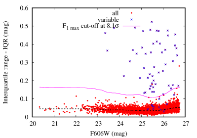
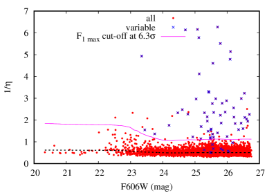
Figure 1: Variability indices characterizing scatter (left panel) and lightcurve smoothness (right panel) plotted as a function of magnitude. The indices are computed for HSC lightcurves of non-variable objects in the M31 halo field 2004AJ….127.2738B . Crosses mark the objects in which artificial non-periodic variability was injected as described in 2017MNRAS.464..274S . Selecting objects above the solid line as candidate variables results in the maximum $F_{1}$-score. Dotted line shows the median value of a variability index as a function of magnitude.

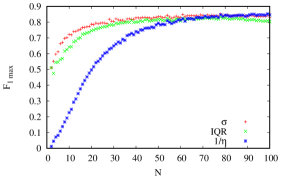
Figure 2: The efficiency of variable objects selection characterized by the maximum (over all possible cut-off thresholds) $F_{1}$-score as a function of the number of lightcurve points, $N$, for three variability indices: $\sigma$, IQR and $1/\eta$ (see the references in Table 1). Based on simulated non-periodic variability injected in HSC lightcurves (M4 field, 2014MNRAS.442.2381N ). For the definition of $F_{1}$-score see https://en.wikipedia.org/wiki/F1_score

Table 1: Variability indices computed by the HCV pipeline.

Index	Errors	Ref.	Index	Errors	Ref.
Indices quantifying lightcurve scatter			time-weighted Stetson’s $J_{\rm time}$	$\checkmark$	2012AJ….143..140F
reduced $\chi^{2}$ statistic – $\chi_{\rm red}^{2}$	$\checkmark$	2010AJ….139.1269D	clipped Stetson’s $J_{\rm clip}$	$\checkmark$	2017MNRAS.464..274S
weighted std. deviation – $\sigma$	$\checkmark$	2008AcA….58..279K	Stetson’s $L$ index	$\checkmark$	1996PASP..108..851S
median abs. deviation – ${\rm MAD}$		2016PASP..128c5001Z	time-weighted Stetson’s $L_{\rm time}$	$\checkmark$	2012AJ….143..140F
interquartile range – ${\rm IQR}$		2017MNRAS.464..274S	clipped Stetson’s $L_{\rm clip}$	$\checkmark$	2017MNRAS.464..274S
robust median stat. – ${\rm RoMS}$	$\checkmark$	2007AJ….134.2067R	consec. same-sign dev. – Con.		2000AcA….50..421W
norm. excess variance – $\sigma_{\rm NXS}^{2}$	$\checkmark$	1997ApJ…476…70N	excursions – $E_{x}$	$\checkmark$	2014ApJS..211….3P
norm. peak-to-peak amp. – $v$	$\checkmark$	2009AN….330..199S	autocorrelation – $l_{1}$		2011ASPC..442..447K
Indices quantifying lightcurve smoothness			inv. von Neumann ratio – $1/\eta$		2009MNRAS.400.1897S
Welch-Stetson index – $I$	$\checkmark$	1993AJ….105.1813W	excess Abbe value – $\mathcal{E}_{\mathcal{A}}$		2014A&A…568A..78M
Stetson’s $J$ index	$\checkmark$	1996PASP..108..851S	$S_{B}$ statistic	$\checkmark$	2013A&A…556A..20F

3 HCV data pre-processing and variability detection pipeline

The HSC data are imported and grouped according to the observed field. The measurements of objects near frame edges or obtained with an old version of the image processing pipeline are excluded as unreliable. For each object all its measurements in a given filter that pass the above selection are collected to construct a lightcurve. Each lightcurve is fitted with a straight line using robust regression and outliers from the fit are identified. If a high percentage of measurements obtained during some visit are identified as outliers in the corresponding lightcurves, all measurements associated with this visit are discarded (bad image). For each of the remaining visits, for each object a local zero-point correction is computed as the mean difference between the measured magnitudes and the ones predicted by the robust line fit for all objects within a specified radius around the object being corrected (Fig. 3). This should compensate for the residual large-scale sensitivity variations across the image.

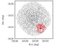
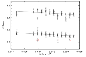
Figure 3: Lightcurve pre-processing. Left: spatial distribution of HSC objects in the M4 field 2014MNRAS.442.2381N . Highlighted are the objects used to determine local magnitude zero-point correction for the object marked with the cross. Right: lightcurve of that object before (top) and after (bottom) applying the local correction. The circles mark identified outlier points. The two lightcurves are shifted along the magnitude axis for clarity.

A set of corrected HSC lightcurves of objects observed in a given field with the same instrument-filter combination is the basic unit of variability search. For each lightcurve in a set we compute variability indices and select as candidate variables the objects that have variability index values significantly higher than the typical value for their brightness. Magnitude-dependent cuts in robust indices IQR and $1/\eta$ are currently used to select candidate variables (Fig. 1). We are investigating ways to efficiently combine information captured by all indices listed in Table 1 by means of the principal component analysis and machine learning.

The HCV pipeline is implemented in Java and parallelized using the Apache Spark framework. The variability indices implementation in the pipeline is consistent with their implementation in VaST (2017arXiv170207715S ) which is also used for lightcurve visualization and testing while a dedicated HCV visualization software is being developed.

4 Summary

• The HCV is a catalog of variable objects derived from the HSC. It will be released in 2018.

• The catalog is very heterogeneous due to the nature of the HSC dataset. It covers selected fields in the Galaxy, the Local Group and beyond.

• The HCV is very deep, it ventures into poorly explored region of variability parameter space.

• Data pre-processing and variability detection techniques used for HCV are applicable to other multi-epoch surveys.

Acknowledgments: This work is supported by ESA under contract No. 4000112940.

References

- (1) Bernard E. J., et al., 2013, MNRAS, 432, 3047
- (2) Brown T. M., Ferguson H. C., Smith E., Kimble R. A., Sweigart A. V., Renzini A., Rich R. M., 2004, AJ, 127, 2738
- (3) Budavári T., Lubow S. H., 2012, ApJ, 761, 188
- (4) de Diego J. A., 2010, AJ, 139, 1269
- (5) Dolphin A. E., et al., 2001, ApJ, 550, 554
- (6) Figuera Jaimes R., Arellano Ferro A., Bramich D. M., Giridhar S., Kuppuswamy K., 2013, A&A, 556, A20
- (7) Fruth T., et al., 2012, AJ, 143, 140
- (8) Gavras P., et al., 2017, arXiv:1703.00258
- (9) Hoffmann S. L., et al., 2016, ApJ, 830, 10
- (10) Jeffery E. J., et al., 2011, AJ, 141, 171
- (11) Kim D.-W., Protopapas P., Alcock C., Byun Y.-I., Khardon R., 2011, ASPC, 442, 447
- (12) Kolesnikova D. M., Sat L. A., Sokolovsky K. V., Antipin S. V., Samus N. N., 2008, AcA, 58, 279
- (13) Lanzerotti L. J., Assessment of options for extending the life of the Hubble Space Telescope: final report (National Academies Press, Washington D.C, 2005)
- (14) Lasker B. M., et al., 2008, AJ, 136, 735
- (15) Mowlavi N., 2014, A&A, 568, A78
- (16) Nandra K., George I. M., Mushotzky R. F., Turner T. J., Yaqoob T., 1997, ApJ, 476, 70
- (17) Nascimbeni V., et al., 2014, MNRAS, 442, 2381
- (18) Parks J. R., Plavchan P., White R. J., Gee A. H., 2014, ApJS, 211, 3
- (19) Rose M. B., Hintz E. G., 2007, AJ, 134, 2067
- (20) Shin M.-S., Sekora M., Byun Y.-I., 2009, MNRAS, 400, 1897
- (21) Sokolovsky K. V., Kovalev Y. Y., Kovalev Y. A., Nizhelskiy N. A., Zhekanis G. V., 2009, AN, 330, 199
- (22) Sokolovsky K. V., et al., 2017, MNRAS, 464, 274
- (23) Sokolovsky K. V., Lebedev A. A., 2017, arXiv:1702.07715
- (24) Stetson P. B., 1996, PASP, 108, 851
- (25) Villforth C., Koekemoer A. M., Grogin N. A., 2010, ApJ, 723, 737
- (26) Welch D. L., Stetson P. B., 1993, AJ, 105, 1813
- (27) Whitmore B. C., et al., 2016, AJ, 151, 134
- (28) Wozniak P. R., 2000, AcA, 50, 421
- (29) Zhang M., Bakos G. Á., Penev K., Csubry Z., Hartman J. D., Bhatti W., de Val-Borro M., 2016, PASP, 128, 035001