Semi-local Exchange Energy Functional For Two-Dimensional Quantum Systems: A Step Beyond Generalized Gradient Approximations

Abstract

Semi-local density functionals for the exchange-correlation energy of electrons are extensively used as it produce realistic and accurate results for finite and extended systems. The choice of techniques play crucial role in constructing such functionals of improved accuracy and efficiency. An accurate and efficient semi-local exchange energy functional in two dimensions is constructed by making use of the corresponding hole based on the density matrix expansion. The exchange hole involved is localized under the generalized coordinate transformation and satisfies all the relevant constraints. Comprehensive testing and excellent performance of the functional is demonstrated versus exact exchange results. The functional also achieves remarkable accuracy by substantially reducing the errors present in the local and non-empirical density functionals proposed so far for two dimensional systems. The underlying principles involved in the functional construction are physically appealing and practically useful for developing range separated and non-local functionals in two dimensions.

Density-functional theory(DFT) hk64 ; ks65 is most successful in addressing the complex effects due to electron-electron interactions. Tremendous advances beyond the local density approximation(LDA) have been achieved through the development of accurate non-local, semi-local and hybrid exchange- correlation(XC) functionals b83 ; jp85 ; pw86 ; b88 ; br89 ; b3pw91 ; pbe96 ; kos ; vsxc98 ; hcth ; tsuneda ; tpss ; mO6l ; revtpss ; tbmbj ; scan15 ; tm16 . However, cutting edge research in low dimensions have also gained momentum as far as the theoretical and experimental findings kat ; rm are concerned. In spite of the promising applications in three dimensions(3D), the dimensional crossover of the XC energy functional from a 3D to two-dimensional(2D) regime, has still remained one of the most difficult open problems klnlhm ; ccfs . Albeit wide use of DFT in 2D still demands potentiality in this direction. So the systematic DFT calculations and proper explanations of numerous properties of low-dimensional systems that range from atomistic to artificial structures e.g., quantum dots, modulated semiconductor layers and surfaces, quantum Hall systems, spintronic devices, quantum rings, and artificial graphene poses great challenge. Thus, the construction of accurate non-local and semilocal XC functionals to appropriately describe systems in 2D is an enthralling and growing research field. In this regard, the first step among the available methods is the well-known 2D-LDA rk . The 2D-LDA combined with the 2D correlation tc ; amgb , lead to intriguing results and establishes its superiority over quantum Monte Carlo simulations hser result. In recent years, advances have been made beyond 2D-LDA e.g., generalized gradient approximations(2D-GGAs) prhg ; prvm ; prg ; pr1 ; prp ; rp ; sr ; pr2 ; rpvm ; prlvm ; vrmp which perform in a more excellent manner. Not only that, several correlation functionals compatible with the 2D-GGAs are also constructed rp ; sr ; pr2 ; rpvm ; prm ; prpg ; rpp .

In principle, the exchange functionals can be constructed from the exchange hole. In 3D, it’s done by making use of Taylor series expansion b83 ; b3pw91 , real space cutoff procedure jp85 , modeling the exchange hole br89 and the density matrix expansion(DME) based on general coordinate transformation kos ; vsxc98 ; hcth ; tsuneda ; mO6l ; tm16 . It is to note that the Taylor series expansion method has been applied to construct 2D-GGA prvm . However, unlike Taylor expansion, DME nv1 ; kos ; vsxc98 ; mO6l ; tm16 based approaches are not only correct for small separation limit, but do converge in the large separation limit tm16 and recover the correct uniform gas behavior. Prompted by these, we have formulated the 2D counterpart of the above DME based exchange energy functional. Advance DME techniques will be proposed for constructing the exchange hole and the corresponding energy functional. Then, the functional will be bench-marked against the optimized effective potential(OEP) based exact- exchange(EXX) kli , local and gradient approximations for 2D systems prvm ; vrmp ; prhg . The OEP based EXX functional is used as reference because it’s the most accurate approach which is routinely applied for studying quantum dots hkprg . Further, the newly constructed functional will be applied to study few electron trapped inside parabolic and Gaussian quantum dots.

The exchange energy is nothing but the electrostatic interaction between the electron located at $\vec{r}$ and the exchange hole at $\vec{r}+\vec{u}$ surrounding it. Thus, the spin-unpolarized exchange functional in 2D is defined as

$$E^{2D}_{x}[\rho]=\frac{1}{2}\int~{}d^{2}r\int\frac{\rho(\vec{r})\rho_{x}(\vec{r},\vec{r}+\vec{u})}{u}~{}d^{2}u,$$ (1)

where $\rho_{x}(\vec{r},\vec{r}+\vec{u})$ be the exchange hole surrounding the electron at $\vec{r}$ and is given by

$$\rho_{x}(\vec{r},\vec{r}+\vec{u})=-\frac{|\varGamma(\vec{r},\vec{r}+\vec{u})|^{2}}{2\rho(\vec{r})}$$ (2)

with the density matrix $\varGamma(\vec{r},\vec{r}+\vec{u})=2\sum_{i}^{occ}\psi_{i}^{*}(\vec{r})\psi_{i}(\vec{r}+\vec{u})$ and the Kohn-Sham (KS) orbitals $\psi_{i}$ . The exchange hole obeys two important properties: (i) the normalization sum rule: $\int~{}\rho_{x}(\vec{r},\vec{r}+\vec{u})~{}d^{2}u=-1$ and (ii) the negativity constraint: $\rho_{x}(\vec{r},\vec{r}+\vec{u})\leq 0$. Now, under general coordinate transformation (i.e. $(\vec{r}_{1},\vec{r}_{2})\to(\vec{r}^{\lambda},u)$), where $\vec{r}^{\lambda}=\lambda\vec{r}_{1}+(1-\lambda)\vec{r}_{2}$, the above exchange functional reduces to

$$E^{2D}_{x}=\frac{1}{2}\int~{}d^{2}r^{\lambda}\rho(\vec{r}^{\lambda})\int\frac{\rho^{t}_{x2D}(\vec{r}^{\lambda},u)}{u}~{}d^{2}u,$$ (3)

where $\rho^{t}_{x2D}$ is the transformed exchange hole defined by

$$\rho^{t}_{x2D}=-\frac{|\varGamma_{1t}^{2D}(\vec{r}^{\lambda}-(1-\lambda)\vec{u},\vec{r}^{\lambda}+\lambda\vec{u})|^{2}}{2\rho(\vec{r})}$$ (4)

with $\varGamma_{1t}^{2D}$ be the KS single particle density matrix. The real parameter, $\lambda$ can take values $1/2\to 1$ (or, $0\to 1/2$). The conventional and on top exchange holes (which is maximally localized in 2D tsp03 ) correspond to $\lambda=1$ and $\lambda=\frac{1}{2}$ respectively. So the transformed single particle KS density matrix around $u=0$ becomes

$$\begin{split}\varGamma_{1t}^{2D}(\vec{r},\vec{u})=e^{\vec{u}.[-(1-\lambda)\vec{\nabla}_{1}+\lambda\vec{\nabla}_{2}]}\varGamma_{1t}^{2D}(\vec{r},\vec{u})|_{\vec{u}=0}\\ =e^{\vec{u}.[-(1-\lambda)\vec{\nabla}_{1}+\lambda\vec{\nabla}_{2}]}\sum_{i}^{occ}\Psi^{*}_{i}(\vec{r}^{\lambda}-(1-\lambda)\vec{u})\Psi_{i}(\vec{r}^{\lambda}+\lambda\vec{u})|_{\vec{u}=0}~{},\end{split}$$ (5)

where $\vec{\nabla}_{1}$ and $\vec{\nabla}_{2}$ operate on $\Psi^{*}_{i}$ and $\Psi_{i}$ respectively. The exchange energy, $E^{2D}_{x}$ involves cylindrical average of the exchange hole $\langle\rho_{x}(\vec{r},\vec{r}+\vec{u})\rangle_{cyl}$ over the direction of $\vec{u}$ i.e.

$$\langle\rho_{x}(\vec{r},\vec{r}+\vec{u})\rangle_{cyl}=\int\rho_{x}(\vec{r},\vec{r}+\vec{u})~{}\frac{d\Omega_{u}}{2\pi}~{}.$$ (6)

On taking the cylindrical average of the density matrix given in Eq.(5) after it’s Taylor series expansion yields the correct small $u$ behavior, i.e.

$$\begin{split}\langle\rho^{t}_{x2D}\rangle=-\frac{\rho(\vec{r})}{2}-\frac{1}{4}\Big{[}\Big{(}\lambda^{2}-\lambda+\frac{1}{2}\Big{)}\nabla^{2}\rho(\vec{r})-2\tau\\ +\frac{1}{4}\Big{(}2\lambda-1\Big{)}^{2}\frac{|\vec{\nabla}\rho(\vec{r})|^{2}}{\rho(\vec{r})}\Big{]}u^{2}~{}.\end{split}$$ (7)

The expression in Eq.(7) was originally proposed for the conventional exchange hole in 3D b83 and then extended to 2D prvm . But, it failed to recover the uniform density limit. In order to recover it, the whole term was multiplied by the exchange hole of uniform electron gas prvm . Whereas, here in this work, all the above deficiencies are accounted through the proposed novel approach based on DME. As a matter of which, it quite rightly obtains: (i) the correct uniform density limit, (ii) the cylindrically averaged exchange hole similar to that given in Eq.(7) when terms up to $u^{2}$ will be considered and (iii) the large $u$-limit (i.e. $0$ to $\infty$ integral limit of $u$) that converges without considering any cutoff procedure. Now, to construct the desired semilocal functional, we begin by considering the DME in Eq.(5) along with the following plane wave expansion in terms of the Bessel and Hypergeometric functions. So

$$e^{\frac{kucos\phi y}{k}}={\mathcal{A}}+{\mathcal{B}}~{},$$ (8)

where

$${\mathcal{A}} = \frac{2}{ku}\sum_{n=0}^{\infty}(-1)^{n}(2n+1)J_{2n+1}(ku)C_{2n}^{1}\Big{(}-i\frac{ycos\phi}{k}\Big{)}$$

$${\mathcal{B}} = \frac{2}{ku^{2}}\sum_{n=0}^{\infty}(-1)^{n}(2n+1)J_{2n+1}(ku)\frac{1}{2\cos\phi}$$ (9)

$$~{}~{}~{}~{}~{}~{}~{}~{}~{}~{}~{}~{}~{}~{}~{}~{}~{}~{}~{}~{}~{}~{}~{}~{}~{}~{}~{}~{}~{}\times\frac{\partial}{\partial y}\Big{[}C_{2n}^{1}\Big{(}-i\frac{ycos\phi}{k}\Big{)}\Big{]}$$

and $\phi$ be the azimuthal angle. The polynomial, $C_{2n}^{m}$ is expressed as

$$C^{m}_{2\nu}(x)=(-1)^{\nu}\begin{pmatrix}\nu+m-1\\ \nu\end{pmatrix}{}_{2}F_{1}(-\nu,\nu+m;\frac{1}{2};x^{2})$$ (10)

with the generalized Hypergeometric function, ${}_{2}F_{1}$, the Bessel function, $J_{2n+1}$ and $y=-(1-\lambda)\vec{\nabla}_{1}+\lambda\vec{\nabla}_{2}$. The series re-summation technique along with the Gegenbauer addition theorem watson are used to arrive at the above expansion (i.e. Eq.(8) and Eq.(9)). Now, Eq.(8) together with Eq.(5) produce the transformed density matrix

$$\varGamma_{1t}^{2D}=2\rho\frac{J_{1}(ku)}{ku}+\frac{6J_{3}(ku)}{k^{3}u}{\mathcal{G}}+\frac{24J_{3}(ku)}{k^{3}u^{2}}{\mathcal{H}}~{},$$ (11)

where

$${\mathcal{G}} = 4\cos^{2}\phi\{(\lambda^{2}-\lambda+\frac{1}{2})\nabla^{2}\rho-2\tau\}+k^{2}\rho$$

$${\mathcal{H}} = \cos\phi(2\lambda-1)|\nabla\rho|$$ (12)

with $\tau=\sum_{i}^{occ}|\vec{\nabla}\psi_{i}|^{2}$, the KS kinetic energy density. Now, to make $\tau$ gauge-invariant, we modify it, so that

$$\tau\to\tilde{\tau}=\tau-2\frac{j_{p}^{2}}{\rho},$$ (13)

where

$$j_{p}=\frac{1}{2i}\sum_{i}^{occ}\{\psi^{*}_{i}(\vec{r})[\vec{\nabla}\psi_{i}(\vec{r})]-[\vec{\nabla}\psi_{i}^{*}(\vec{r})]\psi_{i}(\vec{r})\}$$ (14)

is the para-magnetic current density. By doing this, the functional also becomes gauge invariant and fulfills all the above mentioned criteria. Inclusion of current density is particularly important whenever there happens to be the radiation matter interactions. It is relevant to use the following cylindrical average of the exchange hole (e.g. shown in FIG.1) corresponding to the above density matrix which will be used for the construction of the desired 2D semi-local functional i.e.

$$\langle\rho^{t}_{x2D}\rangle=-\frac{2J_{1}^{2}(ku)}{k^{2}u^{2}}\rho(\vec{r})-\frac{24J_{1}(ku)J_{3}(ku)}{k^{4}u^{2}}{\mathcal{L}}-\frac{144J_{3}^{2}(ku)}{k^{6}u^{4}}{\mathcal{M}}~{},$$ (15)

where

$${\mathcal{L}} = (\lambda^{2}-\lambda+\frac{1}{2})\nabla^{2}\rho-2\tau+4\frac{j_{p}^{2}}{\rho}+\frac{1}{2}k^{2}\rho$$

$${\mathcal{M}} = (2\lambda-1)^{2}\frac{|\nabla\rho|^{2}}{\rho}~{}.$$ (16)

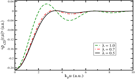
Figure 1: The Eq.(15) is plotted (with $j_{p}=0$) for two non-interacting electrons with density $\rho(r)=\frac{2}{\pi}\exp(-2r^{2})$ parabolically confined in 2D. Shown are the exchange holes at the reference point $r=0.5~{}a.u.$ for several $\lambda$ values, where $r$ be the radial distance from the origin. For $\lambda=1.0$, some portion of the exchange hole is $+ve$ indicating that the exchange hole violates the negativity property and will underestimate the magnitude of exchange energy. This implies the requirement for normalization of exchange hole (see ref. tsp03 for details).

By virtue of the above exchange hole, the functional retains the most unique features like uniform density limit for $k=k_{F}=(2\pi\rho)^{\frac{1}{2}}$ and correct $u^{2}$ behavior. So the above DME based exchange hole is more general in nature than the previously proposed ones prvm . In the earlier case prvm , the small $u$ expansion of cylindrical average exchange hole was multiplied by the corresponding average exchange hole of uniform gas and the parameters were determined using the sum rule. Whereas, in the present attempt, all these are automatically taken care. Thus the uniform density limit is trivially recovered when $k=k_{F}$. But for inhomogeneous systems, the extent of inhomogeneity is included through a parameter $f$ (to be determined analytically) so that $k=fk_{F}$. Then, $f$ is being obtained from the normalization of the cylindrically averaged exchange hole i.e.

$$\frac{1}{f^{2}}+\frac{6}{f^{4}}y=1~{},$$ (17)

where $y=(2\lambda-1)^{2}p$ and $p=s^{2}=\frac{|\vec{\nabla}\rho|^{2}}{(2k_{F}\rho)^{2}}$ is the square of the reduced density gradient in 2D. For slowly varying density limit, Eq.(17) demands that $f\approx 1+6y$ and in the limit of large density gradient, $f\to y^{\frac{1}{4}}$, similar to that proposed in prvm . By applying successive root finding method to solve Eq.(17), we propose that for any arbitrary density the dimensionless parameter $f$ satisfies the relation

$$f=[1+90(2\lambda-1)^{2}p+\beta(2\lambda-1)^{4}p^{2}]^{\frac{1}{15}}~{},$$ (18)

where $\beta$ is the parameter that has to be determined along with $\lambda$ by fitting with exact results known for physical systems. In this case, we found these parameters by comparing with exact exchange results for the few electrons quantum dots. It is noteworthy to mention that in case for low density, the binomial expansion of Eq.(18) leads to $f\approx 1+6y$. Thus, the proposition, Eq.(18) is in right spirit. But the laplacian present in the exchange hole expansion also need to be removed in order to handle it numerically at the origin. The usual way to do so is to use the method of integration by parts. But here, we have used the semi-classical approximation of kinetic energy density bvz to replace it. As this method has been successfully employed in designing the meta-GGA type functional in 3D tpss ; tm16 . So $\nabla^{2}\rho$ is replaced by

$$\nabla^{2}\rho=6\Big{[}\tau-\tau^{unif}_{2D}-2\frac{j_{p}^{2}}{\rho}\Big{]}~{},$$ (19)

where $\tau^{unif}_{2D}=\frac{\pi\rho^{2}}{2}$. Thus, the modified exchange hole takes the form

$$\begin{split}\langle\rho^{t}_{x2D}\rangle=-\frac{2J_{1}^{2}(fk_{F}u)}{f^{2}k_{F}^{2}u^{2}}\rho(\vec{r})-\frac{24J_{1}(fk_{F}u)J_{3}(fk_{F}u)}{f^{4}k_{F}^{4}u^{2}}{\mathcal{L}}\\ -\frac{144J_{3}^{2}(fk_{F}u)}{f^{6}k_{F}^{6}u^{4}}{\mathcal{M}}\end{split}$$

with

$${\mathcal{L}} = 6(\lambda^{2}-\lambda+\frac{1}{2})\Big{[}\tau-\tau^{unif}_{2D}-2\frac{j_{p}^{2}}{\rho}\Big{]}-2\tau+4\frac{j_{p}^{2}}{\rho}+\frac{1}{2}k_{F}^{2}\rho$$

$${\mathcal{M}} = (2\lambda-1)^{2}\frac{|\nabla\rho|^{2}}{\rho}~{}.$$ (20)

Now, from Eq.(1) and Eq.(20), the semilocal exchange energy density functional in 2D is given by

$$E^{2D-mGGA}_{x}=-\int\rho(\vec{r})\epsilon_{x}^{2D-LDA}F_{x}^{2D-mGGA}[p,\tau,j_{p}]~{}d^{2}r~{},$$ (21)

where $\epsilon_{x}^{2D-LDA}=\frac{4k_{F}}{3\pi}$ and the enhancement factor (e.g. shown in FIG.2),

$$F_{x}^{2D-mGGA}[p,\tau,j_{p}]=\frac{1}{f}+\frac{2R}{5f^{3}}$$ (22)

with

$$R = 1+\frac{128}{21}(2\lambda-1)^{2}p$$ (23)

$$+ \frac{3\Big{(}\lambda^{2}-\lambda+\frac{1}{2}\Big{)}\Big{(}\tau-\tau_{2D}^{unif}-2\frac{j_{p}^{2}}{\rho}\Big{)}-\tau+2\frac{j_{p}^{2}}{\rho}}{\tau_{2D}^{unif}}~{}.$$

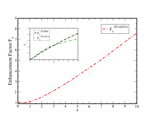
Figure 2: The enhancement factor $F_{x}^{2D-mGGA}$ (with $j_{p}=0$) is plotted as a functional of $s$ for $2$ electrons confined in a parabolic quantum dot with confinement strength $\omega=1$. In the left corner, we have shown the enhancement factors of 2D-GGA prvm and 2D-B88 vrmp for comparison.

Table 1: Shown below are the exchange energies (in atomic units) for parabolically confined few electron quantum dots. The $1^{st}$ and $2^{nd}$ columns contain the number of particles and confinement strengths used for finding the parameters of the proposed functional. Results for EXX, 2D-LDA, 2D-GGA prvm , 2D-B88 vrmp and 2D-BR prhg are also shown for comparison with that obtained using the constructed 2D-mGGA functional. The last row contains the mean percentage error, $\Delta$.

N	$\omega$	$-E_{x}^{EXX}$	$-E_{x}^{LDA}$	$-E_{x}^{GGA}$	$-E_{x}^{B88}$	$-E_{x}^{BR}$	$-E_{x}^{mGGA}$
2	1/6	0.380	0.337	0.368	0.364	0.375	0.386
2	0.25	0.485	0.431	0.470	0.464	0.480	0.492
2	0.50	0.729	0.649	0.707	0.699	0.722	0.735
2	1.00	1.083	0.967	1.051	1.039	1.080	1.085
2	1.50	1.358	1.214	1.319	1.304	1.354	1.354
2	2.50	1.797	1.610	1.748	1.728	1.794	1.776
2	3.50	2.157	1.934	2.097	2.074	2.020	2.113
6	$1/1.89^{2}$	1.735	1.642	1.719	1.749	1.775	1.736
6	0.25	1.618	1.531	1.603	1.594	1.655	1.620
6	0.42168	2.229	2.110	2.206	2.241	2.281	2.226
6	0.50	2.470	2.339	2.444	2.431	2.529	2.466
6	1.00	3.732	3.537	3.690	3.742	3.824	3.716
6	1.50	4.726	4.482	4.672	4.648	4.845	4.699
6	2.50	6.331	6.008	6.258	6.226	6.492	6.279
6	3.50	7.651	7.264	7.562	7.525	7.846	7.573
12	0.50	5.431	5.257	5.406	5.387	5.728	5.415
12	1.00	8.275	8.013	8.230	8.311	8.572	8.231
12	1.50	10.535	10.206	10.476	10.444	10.915	10.461
12	2.50	14.204	13.765	14.122	14.080	14.716	14.063
12	3.50	17.237	16.709	17.136	17.086	17.858	17.019
20	0.50	9.765	9.553	9.746	9.722	10.167	9.805
20	1.00	14.957	14.638	14.919	15.029	15.573	14.894
20	1.50	19.108	18.704	19.053	19.188	19.892	19.007
20	2.50	25.875	25.334	25.796	25.973	26.935	25.698
20	3.50	31.491	30.837	31.392	31.603	32.777	31.230
$\Delta$			5.7	1.7	3.9	2.8	0.7

To test the functional and obtain the parameters $\beta$ and $\lambda$, we have chosen the set of parabolic quantum dots having varying confinement strengths with few electrons embedded into it. This type of system is reported for testing the 2D-GGA functional prvm and to fix the corresponding parameters involved therein. A self-consistent calculation with KLI-OEP exact-exchange method using OCTOPUS code octopus has been performed and the density is being used as the reference input. As our system is non-magnetic, so $j_{p}=0$. The value of $\lambda$ is obtained by fitting with different confinement strengths such that the mean percentage error gets reduced. Whereas, $\beta$ is fixed so as to confirm the smooth behavior of the enhancement factor in the $s\approx 0$ region ptss04 . The value of the parameters $\lambda$ and $\beta$ are obtained to be $0.74$ and $30.0$ respectively. In $3D$ tm16 , same set of parameters are also used. But those are fixed by taking the exact exchange of hydrogen atom along with the smooth behavior of the enhancement factor at the iso-orbital region in order to remove the spurious divergence of the exchange potential ptss04 . The current functional is tested and the performance of it is shown in Table-I. Trivially, the results are quite superior as it yields error that are smaller by at least a factor of $8.1$, $2.4$, $5.6$ and $4.0$ w.r.t. 2D-LDA, 2D-GGA prvm , 2D-B88 vrmp and 2D-BR prhg respectively. Lastly, the comprehensive assessment of the functional is being performed for Gaussian quantum dots by simultaneously varying the the number of electrons trapped $N$, depth of the potential and confinement strength $\omega$. For this case, the performance is presented in Table-II and FIG.3. Here too, the results are found to be in excellent agreement with KLI-EXX. Actually, the new semilocal functional reduces the error by a factor of $2.2$ compared to 2D-GGA for the whole set.

Table 2: Comparison of exchange energies (a.u.) for Gaussian quantum dots ($v_{ext}=-V_{0}e^{-\omega^{2}r^{2}})$ are shown for low density. Mean percentage error given in the last row.

$V_{0}$	N	$\omega^{2}$	$-E_{x}^{EXX}$	$-E_{x}^{LDA}$	$-E_{x}^{GGA}$	$-E_{x}^{mGGA}$
10	2	0.05	1.047	0.934	1.017	1.048
10	2	0.10	1.255	1.120	1.219	1.250
10	2	0.25	1.573	1.405	1.529	1.555
10	2	1/6	1.427	1.274	1.386	1.416
10	2	0.50	1.839	1.643	1.788	1.804
40	6	0.05	5.416	5.139	5.354	5.372
40	6	0.10	6.525	6.194	6.450	6.460
40	6	0.25	8.255	7.840	8.160	8.142
40	6	1/6	7.454	7.076	7.367	7.364
$\Delta$				8.3	2.0	0.9

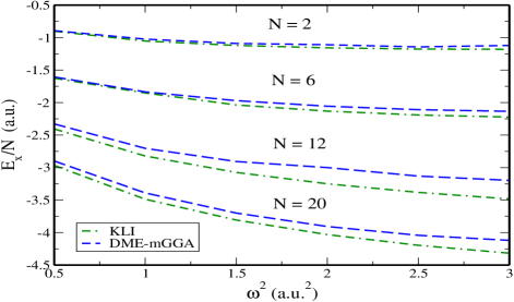
Figure 3: Shown in the figure, the exchange energy per electron (in a.u.) plotted versus $\omega^{2}$ for a series of Gaussian quantum dots with $N$ electrons and confinement strength $\omega$.

To summarize, a meta-GGA type semi-local functional in two dimensions is constructed based on DME. The beauty of this functional is that, the exchange hole involved in it has correct short range behavior and recovers the uniform density limit quite accurately. The convergence of the exchange hole in large separation limit leads to an analytical expression for the corresponding energy functional even without applying any cutoff procedure which are essentially lacked by 2D functionals proposed so far. The most appealing feature of the present semi-local functional is that it is derived from the full exchange hole and thus having strong physical basis. The functional is one step ahead of the 2D-GGA as it leads to significant reduction in error compare to it’s counterparts. Thus, the functional in principle can enable us for making precise many-electron calculations of larger structures such as arrays of quantum-dots, quantum-Hall devices, semiconductor quantum dots, quantum Hall bars on a regular basis. Also, the constructed exchange hole can be used to construct meta-GGA level exchange only pair-distribution function, static structure factor, non-local and range separated functionals in 2D. The present construction can be further extended to the recently developed density functional formalism for strictly correlated electrons. The next step is to construct functional for correlation energy which will be compatible with the exchange. The functional is not only physically appealing but also practically useful as it opens the path for constructing exchange correlation functionals in two dimensions analogue to the Jacob’s ladder in three dimensions.

The authors would like to acknowledge the financial support from the Department of Atomic Energy, Government of India.

References

- (1) P. Hohenberg and W. Kohn, Phys. Rev. 136, B864 (1964).
- (2) W. Kohn and L. J. Sham, Phys. Rev. 140, A1133 (1965).
- (3) A. D. Becke, Int. J. Quant. Chem. 23, 1915 (1983).
- (4) J. P. Perdew, Phys. Rev. Lett. 55, 1665 (1985)
- (5) J. P. Perdew and Y. Wang, Phys. Rev. B 33, 8800 (1986).
- (6) A. D. Becke, Phys. Rev. A 38, 3098 (1988).
- (7) A. D. Becke and M. R. Roussel, Phys. Rev. A 39, 3761 (1989).
- (8) A. D. Becke, J. Chem. Phys. 104, 1040 (1996).
- (9) J. P. Perdew, K. Burke and M. Ernzerhof, Phys. Rev. Lett. 77, 3865 (1996).
- (10) R. M. Koehl, G. K. Odom and G. E. Scuseria, Mol. Phys. 87, 835 (1996).
- (11) T. V. Voorhis and G. E. Scuseria, J. Chem. Phys. 109, 400 (1998).
- (12) F. A. Hamprecht, A. J. Cohen, D. J. Tozer and N. C. Handy, J. Chem. Phys. 109, 6264 (1998).
- (13) T. Tsuneda and K. Hirao, Phys. Rev. B 62, 15527 (2000).
- (14) J. Tao, J. P. Perdew, V. N. Staroverov and G. E. Scuseria, Phys. Rev. Lett. 91, 146401 (2003).
- (15) Y. Zhao and D. G. Truhlar, J. Chem. Phys. 125, 194101 (2006).
- (16) J. P. Perdew, A. Ruzsinszky, G.I. Csonka, L. A. Constantin and J. Sun, Phys. Rev. Lett. 103, 026403 (2009).
- (17) F. Tran and P. Blaha, Phys. Rev. Lett. 102, 226401 (2009).
- (18) J. Sun, A. Ruzsinszky and J.P. Perdew, Phys. Rev. Lett. 115, 036402 (2015).
- (19) J. Tao and Y. Mo, Phys. Rev. Lett. 117, 073001 (2016).
- (20) L. P. Kouwenhoven, D. G. Austing and S. Tarucha, Rep. Prog. Phys. 64, 701 (2001).
- (21) S. M. Reimann and M. Manninen, Rev. Mod. Phys. 74, 1283 (2002).
- (22) Y. -H. Kim, I. -H. Lee, S. Nagaraja, J.-P. Leburton, R. Q. Hood and R. M. Martin, Phys. Rev. B 61, 5202 (2000).
- (23) L. Chiodo, L. A. Constantin, E. Fabiano and F. Della Sala, Phys. Rev. Lett. 108, 126402 (2012).
- (24) A. K. Rajagopal and J. C. Kimball, Phys. Rev. B 15, 2819 (1977).
- (25) B. Tanatar and D. M. Ceperley, Phys. Rev. B 39, 5005 (1989).
- (26) C. Attaccalite, S. Moroni, P. Gori-Giorgi and G. B. Bachelet, Phys. Rev. Lett. 88, 256601 (2002).
- (27) H. Saarikoski, E. Räsänen, S. Siljamäki, A. Harju, M. J. Puska and R. M. Nieminen, Phys. Rev. B 67, 205327 (2003).
- (28) S. Pittalis, E. Räsänen, N. Helbig and E. K. U. Gross, Phys. Rev. B 76, 235314 (2007).
- (29) S. Pittalis, E. Räsänen, J. G. Vilhena and M. A. L. Marques, Phys. Rev. A 79, 012503 (2009).
- (30) S. Pittalis, E. Räsänen and E. K. U. Gross, Phys. Rev. A 80, 032515 (2009).
- (31) S. Pittalis and E. Räsänen, Phys. Rev. B 80, 165112 (2009).
- (32) S. Pittalis, E. Räsänen and C. R. Proetto, Phys. Rev. B 81, 115108 (2010).
- (33) E. Räsänen and S. Pittalis, Physica E 42, 1232–1235 (2010).
- (34) S. Sakiroglu and E. Räsänen, Phys. Rev. A 82, 012505 (2010).
- (35) S. Pittalis and E. Räsänen, Phys. Rev. B 82, 165123 (2010).
- (36) E. Räsänen, S. Pittalis, J. G. Vilhena and M. A. L. Marques, Int. J. Quant. Chem. 110, 2308–2314 (2010).
- (37) A. Putaja, E. Räsänen, R. van Leeuwen, J. G. Vilhena and M. A. L. Marques, Phys. Rev. B 85, 165101 (2012).
- (38) J. G. Vilhena,E. Räsänen, M. A. L. Marques and S. Pittalis, J. Chem. Th. Comp. 10, 1837−1842 (2014).
- (39) S. Pittalis, E. Räsänen and M. A. L. Marques, Phys. Rev. B 78, 195322 (2008).
- (40) S. Pittalis, E. Räsänen, C. R. Proetto and E. K. U. Gross, Phys. Rev. B 79, 085316 (2009).
- (41) E. Räsänen, S. Pittalis and C. R. Proetto, Phys. Rev. B 81, 195103 (2010).
- (42) J. W. Negele and D. Vautherin, Phys. Rev. C 5, 1472 (1972).
- (43) J. B. Krieger, Y. Li, and G. J. Iafrate, Phys. Rev. A 46, 5453 (1992).
- (44) N. Helbig, S. Kurth, S. Pittalis, E. Räänen and E. K. U. Gross, Phys. Rev. B 77, 245106 (2008).
- (45) J. Tao, M. Springborg and J. P. Perdew, J. Chem. Phys. 119, 6457 (2003).
- (46) G. N. Watson, A Treatise on the Theory of Bessel Functions, New York: Macmillan, (1944).
- (47) M. Brack and B. P. van Zyl, Phys. Rev. Lett. 86, 1574 (2001).
- (48) M. A. L. Marques, A. Castro, G. F. Bertsch and A. Rubio, Comp. Phys. Comm. 151, 60 (2003).
- (49) J. P. Perdew, J. Tao, V. N. Staroverov and G.E. Scuseria, J. Chem. Phys. 120, 6898 (2004).