Using Graphs of Classifiers to Impose Declarative Constraints on Semi-supervised Learning

Abstract

We propose a general approach to modeling semi-supervised learning (SSL) algorithms. Specifically, we present a declarative language for modeling both traditional supervised classification tasks and many SSL heuristics, including both well-known heuristics such as co-training and novel domain-specific heuristics. In addition to representing individual SSL heuristics, we show that multiple heuristics can be automatically combined using Bayesian optimization methods. We experiment with two classes of tasks, link-based text classification and relation extraction. We show modest improvements on well-studied link-based classification benchmarks, and state-of-the-art results on relation-extraction tasks for two realistic domains.

1 Introduction

Most semi-supervised learning (SSL) methods operate by introducing “soft constraints” on how a learned classifier will behave on unlabeled instances, with different constraints leading to different SSL methods. For example, logistic regression with entropy regularization Grandvalet and Bengio (2004) and transductive SVMs Joachims (1999) constrain the classifier to make confident predictions at unlabeled points, and similarly, many graph-based SSL approaches require that the instances associated with the endpoints of an edge have similar labels or embeddings Belkin et al. (2006); Talukdar and Crammer (2009); Weston et al. (2012); Zhou et al. (2003); Zhu et al. (2003). Other weakly-supervised methods also can be viewed as imposing constraints on predictions made by a classifier: for instance, in distantly-supervised information extraction, a useful constraint requires that the classifier, when applied to the set $S$ of mentions of an entity pair that is a member of relation $r$, classifies at least one mention in $S$ as a positive instance of $r$ Hoffmann et al. (2011).

Here we propose a general approach to modeling SSL constraints. We will define a succinct declarative language for specifying semi-supervised learners. We call our declarative SSL framework the D-Learner.

As observed by previous researchers Zhu (2005), the appropriate use of SSL is often domain-specific. The D-Learner framework allows us to define various constraints easily. Combined with a tuning strategy with Bayesian Optimization, we can collectively evaluate the effectiveness of these constraints so as to obtain tailor-made SSL settings for individual problems. To examine the efficacy of D-Learner, we apply it to two tasks: link-based text classification and relation extraction. For the link-based classification task, we will show the flexibility of our declarative language by defining several SSL constraints for exploiting network structures. For the relation extraction task, we will show how our declarative language can express several intuitive problem-specific SSL constraints. Comparison against existing SSL methods Hoffmann et al. (2011); Bing et al. (2017); Surdeanu et al. (2012) shows that D-Learner achieves significant improvements over the state-of-the-art on two domains.

2 D-Learner: Declaratively Specifying Constraints for Semi-supervised Learners

2.1 An Example: Supervised Classification

predict(X,Y) $\leftarrow$ pickLabel(Y) $\wedge$ classify(X,Y). classify(X,Y) $\leftarrow$ true $\{$ f(W,Y): hasFeature(X,W) $\}$.    mutexFailure(X) $\leftarrow$ pickMutex(Y1,Y2) $\wedge$ classify(X,Y1) $\wedge$ classify(X,Y2).

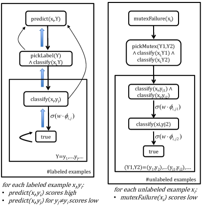
Figure 1: Declarative specifications of the models for supervised learning, on the left, and for a mutual-exclusivity constraint, on the right.

Figure 2: Plate diagrams for supervised learning on the left, and a mutual-exclusivity constraint on the right.

We begin with a simple example. The left-hand side of Figure 2 illustrates how traditional supervised classification can be expressed declaratively in a logic program. Following the conventions used in logic programming, capital letters are universally quantified variables. We extend traditional logic programs by allowing rules to be annotated with a set of features, which will be then weighted to define a strength for the rule (as we will describe below). The symbol true is a goal that always succeeds.

D-learner programs are associated with a backward-chaining proof process, can be read either as logical constraints, or as a non-deterministic program, which is invoked when a query is submitted. If the queries processed by the program are all of the form predict($x_{i}$,Y) where $x_{i}$ is a constant, the theory on the left-hand side of Figure 2 can be interpreted as saying: (1) To prove the goal of the form predict($x_{i}$,Y)—i.e., to predict a label $Y$ for the instance $x_{i}$—non-deterministically pick a possible class label $y_{j}$, and then prove the goal classify($x_{i}$,$y_{i}$); (2) proofs for every the goal classify($x_{i}$,$y_{j}$) immediately succeed, with a strength based on a weighted combination of the features in the set $\{f(w,y_{j}):hasFeature(x_{i},w)\}$. This set is encoded in the usual way as a sparse vector $\phi_{x_{i},y_{j}}$, with one dimension for every object of the form $f(w,y_{j})$ where $y_{j}$ is a class label and $w$ is a vocabulary word. For example, if the vocabulary contains the word hope and sports is a possible label, then one feature in $\phi_{x_{i},y_{j}}$ might be active exactly when document $x_{i}$ contains the word $hope$ and $y_{j}=\textit{sports}$. The set of proofs associated with this theory are described by the plate diagram on the left-hand side of Figure 2, where the upward-pointing blue arrows denote logical implication, and the repetition suggested by the plates has the same meaning as in graphical models. The black arrows will be explained below.

2.2 Semantics of D-Learner Constraints

The D-learner constraints are implemented in a logic programming language called ProPPR Wang et al. (2013), whose semantics are defined by a slightly different graph. The ProPPR graph contains the same set of nodes as the proof graph, but is weighted, and has a different edge set—namely, the downward-pointing black arrows, which run opposite to the implication edges. For this example, these edges describe a forest, with one tree for each labeled example $x_{i}$. Each tree in the forest begins branching at distance two from the root, and will have $N$ nodes labeled true where $N$ is the number of possible class labels. The forest is further augmented with some additional edges: in particular, we will add a self-loop to each true node, and a “reset” edge that returns to the root (the curved upward-pointing arrows) for each non-true node. (To simplify, the reset and self-loop edges are only shown in the first plate diagram.) The light upward-pointing edges will have an implicit weight of $\alpha$, for some fixed $0<\alpha<1$, unannotated edges have an implicit weight of one, and the weight of feature-annotated edges will be discussed below. Finally, if feature vector $\phi$ is associated with a rule, then the edges produced using that rule are annotated with the feature vector. (We abbreviate $\phi_{x_{i},y_{j}}$ with $\phi_{i,j}$ in the figure.) The weight of such an edge is $\sigma(\mathbf{w}\cdot\phi_{i,j})$, where $\mathbf{w}$ is a learned parameter vector, and $\sigma$ is a nonlinear “squashing” function (e.g., $\sigma(x)\equiv\frac{1}{1+e^{-x}}$). In the example, these edges are the ones that exit a node labeled classify($x_{i}$,$y_{j}$). These are labeled with the function $\sigma(\mathbf{w}\cdot\phi_{i,j})$, and recall that the vector $\phi_{i,j}$ encodes features associated with the document $x_{i}$ with the label $y_{j}$.

We can now define a Markov process, based on repeatedly transitioning from a node $v$ to its neighbors, using the normalized outgoing edges of $v$ as a transition function. This process is well-defined for any set of positive edge weights (and positivity can be ensured by the choice of $\sigma$) and any graph architecture, and will assign a probability score $\pi_{w}(v)$ to every node $v$. Conceptually, it can be viewed as a probabilistic proof process, with the “reset” corresponding to abandoning a proof Wang et al. (2013).

Imagine that $\mathbf{w}$ has been trained so that for an example $x_{i}$ with true label $y_{j*}$, $\mathbf{w}\cdot\phi_{i,j*}$ has the largest score over all the possible labels $y_{j}$. Note that every true node corresponds to a label $y_{j}$. It is not hard to see that the ordering of $\pi(v)$ over the true nodes in the graph for $x_{i}$ maintains a close correspondence to classification performance. In particular, even though the graph is locally normalized, the $\phi_{i,j}$-labeled edges compete with the upward-pointing “reset” edges that lead to the root, so a larger weight will direct more of the probability mass of the walk toward the true node associated with label $j*$. More specifically, the true node associated with label $y_{j*}$ will have the highest $\pi$ of any true node in the graph. Thus, in the example, there is a close connection between the problem of setting $\mathbf{w}$ to minimize empirical loss of the classifier, and setting $\mathbf{w}$ to satisfy constraints on the Markov-walk scores of the nodes in the graph.

In ProPPR, it is possible to train weights to maximize or minimize the score of a particular query response: i.e., one can say that for the query predict($x_{i},Y$) responses where $Y=y_{j*}$ are “positive” and responses where $Y=y_{j^{\prime}}$ for $j^{\prime}\not=j*$ are “negative”. Specifically a positive example $a$ incurs a loss of $\log_{\sum_{v\in{}V}\pi(v)}$, where $V$ is the set of true nodes that support answer $a$, and a negative example incurs a loss of $\log_{1-\sum_{v\in{}V}\pi(v)}$. The training data needed for the supervised learning case is indicated in the bottom of the left-hand of the plate diagram. Learning is performed by stochastic gradient descent Wang et al. (2013).

2.3 An example: Semi-supervised Learning

We finally turn to the right-hand parts of Figures 2 and 2, which are a D-learner specification for an SSL method. These rules are a consistency test to be applied to each unlabeled example $x_{i}$. In ordinary classification tasks, any two distinct classes $y_{j}$ and $y_{j^{\prime}}$ should be mutually exclusive. The theory on the right-hand side of Figure 2 asserts that a “mutual exclusion failure” (mutexFailure) occurs if $x_{i}$ can be classified into two distinct classes. The corresponding plate diagram is shown in Figure 2, simplified by omitting the “reset” edges and the self-loops on true nodes. To (softly) enforce this constraint, we need only to introduce negative examples for each unlabeled example $x_{i}$, specifying that proofs for the goal mutexFailure($x_{i}$) should have low scores.

Conceptually, this constraint encodes a common bias of SSL systems: the decision boundaries should be drawn in low-probability regions of the space. For instance, transductive SVMs maximize the “unlabeled data margin” based on the low-density separation assumption that a good decision hyperplane lies on a sparse area of the feature space Joachims (1999). In this case, if a decision boundary is close to an unlabeled example, then more than one classify goals will succeed with a high score.

3 Link-based Classification with D-Learner

The example above explains in detail how to specify one particular type of constraint which is widely used in the past SSL works. Of course, if this was the only type of constraint that could be specified, D-Learner would not be of great interest: the value of D-Learner is that it allows one to succinctly specify (and implement) many other plausible constraints that can potentially improve learning. Here we show its application in the task of link-based text classification.

3.1 The Task and Constraints

Many real-world datasets contain interlinked entities (e.g. publications linked by citation relation) and exhibit correlations among labels of linked entities. Link-based classification aims at improving classification accuracy by exploiting such link structures besides the attribute values (e.g., text features) of each entity. In this task, we classify each publication into a pre-defined class, e.g. Neural_Networks. Each publication has features in two views: text content view and citation view. Thus, each publication can be represented as features of its terms or features of its citations.

Similar to the classifier defined above, we have the text view classifier:
predictT(X,Y) $\leftarrow$pickLabel(Y) $\wedge$classifyT(X,Y). classifyT(X,Y) $\leftarrow$ true    $\{$ f(W,Y): hasFeature(X,W) $\}$.

And the citation view classifier:
predictC(X,Y) $\leftarrow$pickLabel(Y) $\wedge$classifyC(X,Y). classifyC(X,Y) $\leftarrow$ true    $\{$ g(Cited,Y): cites(X,Cited) $\}$.

Mutual-exclusivity constraints mutexFailureT and mutexFailureC of the text and citation classifiers are defined in the same way as done in Section 2.3.

Cotraining constraints. D-Learner coordinates the classifiers of two views to make consistent predictions on testing data by imposing penalty when they disagree:
coFailure(X) $\leftarrow$ pickMutex(Y1,Y2) $\wedge$classifyT(X,Y1) $\wedge$                      classifyC(X,Y2). coFailure(X) $\leftarrow$ pickMutex(Y1,Y2) $\wedge$classifyC(X,Y1) $\wedge$                      classifyT(X,Y2).

Table 1: Datasets for link-based classification task.

	CiteSeer	Cora	PubMed
# of publications	3,312	2,708	19,717
# of citation links	4,732	5,429	44,338
# classes	6	7	3
# of unique words	3,703	1,433	500

Propagation constraints. An initial narrative of label propagation (LP) algorithms is that the neighbors of a good labeled example should be classified consistently with it. To express this in the text view, D-Learner penalizes the violators by:
lpFailure1(X,Y) $\leftarrow$ sim1(X,Z)$\wedge$pickMutex(Y,!Y)$\wedge$predictT(Z,!Y).

where pickMutex(Y,!Y) can be replace with pickMutex(!Y,Y) to get another constraint, and sim1 is defined as:
sim1(X1,X2) $\leftarrow$ near(X1,Z)$\wedge$sim1(Z,X2). sim1(X,X) $\leftarrow$ true.

If X1 cites or is cited by Z, then near(X1,Z) is true. Thus, lpFailure1 encourages the publications that have a citation path to X to take the same label as X.

Extending the above one-step walk based sim1 clause, we define a “two-step” walk based one:
sim2(X1,X2) $\leftarrow$ near(X1,Z1)$\wedge$near(Z1,Z2)$\wedge$sim2(Z2,X2). sim2(X,X) $\leftarrow$ true.

Accordingly, the constraint using sim2 is referred to as lpFailure2. It encourages the publications cite or are cited by the same publication to have the same label.

Regularization constraints. D-Learner can implement the well-studied regularization technique in SSL by smoothing the behavior of a classifier on unlabeled data. Specifically, for an unlabeled example, we smooth its label and its neighbors’ labels by:
smoothFailure(X1) $\leftarrow$ pickMutex(Y1,Y2)$\wedge$              classifyT(X1,Y1)$\wedge$near(X1,X2)$\wedge$classifyT(X2,Y2).

3.2 Experiments

3.2.1 Settings

We use three datasets from Sen et al. (2008): CiteSeer, Cora and PubMed, with their statistical information given in Table 1. For each dataset, we use 1,000 publications for testing, and at most 5,000 publications for training. Among the training publications, we randomly pick 20 as labeled examples for each class, and the remaining ones are used as unlabeled. After the examples are prepared, we employ ProPPR to learn multi-class classifiers with $\alpha=0.1$. The maximum epoch number is 40, and we find the training usually converges in less than 10 epochs. Note that constraints are combined with equal weights, and we control the effect of different constraints by using different numbers of examples from them (details discussed later).

3.2.2 Results

We compare with two supervised learning baselines: SL-SVM and SL-ProPPR, which only employ the text view features to train classifiers with SVMs and ProPPR, respectively. For SL-SVM, a linear kernel is used to train multi-class classifiers. Another compared baseline is SSL-naive, which simply uses all examples of all constraints in the semi-supervised learning, regardless their actual effects. D-Learner invokes a tuning strategy to determine how to use the constraints.

We employ accuracy as the evaluation metric, which is defined as the ratio between the number of correct predictions and the number of total predictions (i.e. the number of testing examples). The results are given in Table 2. D-Learner consistently outperforms SL-ProPPR on all three datasets, and the relative improvements are about 1.5% to 5%. Compared with SL-SVM, D-Learner achieves better results on the Cora and PubMed datasets, with relative improvements about 12% and 6%, respectively. For the CiteSeer dataset, D-Learner’s performance is comparable to SL-SVM. Although each constraint has its own intuitive interpretation, SSL-naive does not perform well, particularly poor on CiteSeer and Cora, which suggests that the appropriate use of SSL is often domain-specific Zhu (2005), and needs more careful assessment on the heuristics.

Table 2: Link-based classification results.

	CiteSeer	Cora	PubMed
SL-SVM	0.558	0.520	0.665
SL-ProPPR	0.528	0.551	0.688
SSL-naive	0.109	0.334	0.672
D-Learner	0.551	0.581	0.699

3.2.3 Tuning with Bayesian Optimization

To exploit how to use those domain-specific constraints, D-Learner incorporates a Bayesian optimization based tuning method Snoek et al. (2012), in which a learning algorithm’s generalization performance is modeled as a sample from a Gaussian process. The released package, Spearmint, allows one to program a wrapper for the communication with the tuned algorithm, while searching the optimal parameters. Specifically, the wrapper passes the parameters suggested by Spearmint into the learning algorithm, then collects the results from the algorithm for Spearmint to generate a new suggestion.

Instead of adding a weight to control one constraint’s effect, we adopt a more straightforward way which tunes the example number of a constraint to use. Thus, we have 6 parameters: the example numbers of coFailure (#cF), lpFailure1 (#lpF1), lpFailure2 (#lpF2), mutexFailureT (#mFT), mutexFailureC (#mFC), and smoothFailure (#sF), as listed in Table 3. lpFailure2 is found helpful on all three datasets. The mutual-exclusivity constraint of text view is helpful on Cora and PubMed datasets. Cotraining classifiers of both citation view and text content view does not improve the results, it is because, in the three datesets, the average citation number of publications is about 1.5 to 2.5, which is too sparse to train a reliable citation view classifier.

4 Relation Extraction with D-Learner

4.1 The Task

We note that in many NLP tasks, there are a plausible number of task-specific constraints which can be easily formulated by a domain expert. In this section we will describe a number of constraints of relation extraction for entity-centric corpora. Each document in an entity-centric corpus describes aspects of a particular entity (called subject or title entity), e.g. each Wikipedia article is such a document. Relation extraction from an entity-centric document is reduced to predicting the relation between the subject entity (i.e. the first argument of the relation) and an entity mention (i.e. the second argument) in the document. For example, from a drug article “Aspirin”, if the target relation is “sideEffects”, we need to predict for each candidate (extracted from a single sentence) whether it is a side effect of “Aspirin”. If no such relation holds, we predict the special label “Other”. This task in medical domain was initially proposed in Bing et al. (2016, 2017), where a reader could find more details.

Table 3: Parameter tuning for link-based classification.

	Citeseer		Cora		PubMed
	Range	Optimal	Range	Optimal	Range	Optimal
#cF	[0, 2,192]	0	[0, 1,568]	0	[0, 4,940]	0
#lpF1	[0, 120]	0	[0, 140]	0	[0, 60]	0
#lpF2	[0, 120]	80	[0, 140]	140	[0, 60]	60
#mFT	[0, 2,192]	0	[0, 1,568]	1,568	[0, 4,940]	4,940
#mFC	[0, 2,192]	0	[0, 1,568]	0	[0, 4,940]	0
#sF	[0, 2,192]	0	[0, 1,568]	0	[0, 4,940]	0

4.2 Co-training Relation and Type Classifiers

The second argument of a relation is usually of a particular unary type. For example, the second argument of the “interactsWith” relation is always a drug. Therefore, a plausible idea is to impose an agreement constraint between relation and type classifiers, analogous to enforcing agreements between classifiers of different views.

With our declarative language, we can coordinate the tasks of predicting relation and type as follows:
coFailure(X)$\leftarrow$ predictR(X,Y)$\wedge$pickRealLabel(Y)$\wedge$             inRangeT(Y,T1)$\wedge$pickMutexT(T1,T2)$\wedge$predictT(X,T2),

where pickRealLabel(Y) consists of trivial rules for each non-“Other” relation label, and inRangeT(Y,T1) consists of trivial rules for each relation label and its value range type, pickMutexT(T1,T2) consists of trivial rules of each distinct pair of type labels, predictR and predictT are relation and type classifiers, respectively. In other words, coFailure($x_{i}$) says we should penalize cases where a mention $x_{i}$ is predicted having the real relation label Y (i.e. not “Other”), whose range is type T1, but the predicted type of $x_{i}$ is T2 which is mutually exclusive with T1. Thus, by specifying that proofs for the goal coFailure($x_{i}$) having low scores, classifiers that make this sort of error will be downweighted.

Mutual-exclusivity constraints mutexFailureT and mutexFailureR of type and relation classifiers are defined in the same way as we did before.

4.3 SSL Constraints for Relation Extraction

Document constraint. If an entity string appears as multiple mentions in a document, they should have the same relation label (relative to the subject), or some have “Other” label:
docFailure(X1,X2) $\leftarrow$ pickMutex(Y1,Y2)$\wedge$pickRealLabel(Y1)$\wedge$             pickRealLabel(Y2)$\wedge$classify(X1,Y1)$\wedge$classify(X2,Y2).

For example, if “heartburn” appears twice in the “Aspirin” document, we should make consistent predictions, i.e. “sideEffects” for them, or predict one or both as “Other”. Note that a mention can also refer to a coordinate-term list, such as “vomiting, headache and nausea”, of multiple NPs. In fact, we compute the intersection of the NP sets of two mentions, and if it is not empty, this constraint applies, such as for “vomiting, and headache” and “vomiting, and heartburn”.

Sentence constraint. For each sentence, we require that only one mention can be labeled as a particular relation (this requirement is usually satisfied in real data):
sentFailure(X1,X2) $\leftarrow$ pickRealLabel(Y1)$\wedge$pickRealLabel(Y2)$\wedge$                       classify(X1,Y1)$\wedge$classify(X2,Y2),

where X1 and X2 are a pair of mentions extracted from a single sentence. This constraint penalizes extracting multiple relation objects from a single sentence. For example, from the sentence “Some products that may interact with this drug include: Aliskiren and ACE inhibitors”, “some products” and “Aliskiren and ACE inhibitors” should not be labeled as the interactsWith relation simultaneously.

Section title constraint. In some entity-centric corpora, the content of a document is organized into sections. This constraint basically says, for two mentions of the same NP in the same section (currently determined simply by matching section titles) of two documents, they should have the same relation label, relative to their own document subjects:
titleFailure(X1,X2) $\leftarrow$ pickMutex(Y1,Y2)$\wedge$pickRealLabel(Y1)$\wedge$              pickRealLabel(Y2)$\wedge$classify(X1,Y1)$\wedge$classify(X2,Y2).

E.g., if “heartburn” appears in “Adverse reactions” sections of drugs “Aspirin” and “Singulair”, it is plausible to infer both mentions are “sideEffects”, or one or both are “Other”.

4.4 Experiments

4.4.1 Settings

We follow the experimental settings in Bing et al. (2017). The drug corpus is DailyMed containing 28,590 articles, and the disease corpus is WikiDisease containing 8,596 articles. 3 and 5 relations are extracted for drugs and diseases, respectively. A pipeline’s task then is to extract all correct values of the second argument of a given relation from a test document. The range types of the second arguments of relations are also defined in their paper. For details about preprocessing, features, distant labeling seeds, annoated evaluation and tuning datasets, please refer to Bing et al. (2017).

4.4.2 Training Classifiers

Without manually labeled training relation examples, we employ the seed triples from Freebase to distantly label articles in the corpora, as done in Bing et al. (2017). For instance, the triple sideEffects(Aspirin,heartburn) will label a mention “heartburn” from the Aspirin article as an example of sideEffects relation. The raw data by distant labeling is very noisy Riedel et al. (2010); Bing et al. (2015, 2016, 2017), so we employ the distillation method with LP in Bing et al. (2017) to get a cleaner set of relation examples, where the top K (the tuning for K will be described later) most confident, scored by LP, examples are used as training data. We also pick a set of mentions from the testing corpus that are not labeled as any relation as general negative examples.

The training type examples are collected by DIEL Bing et al. (2015), which extracts the instances of those range types from Freebase as seeds, and extends the seed set by LP. After that, we pick top K as training examples. Similarly, we also randomly pick a number of general negative type examples.

4.4.3 Compared Baselines

We compare against three existing methods: MultiR, Hoffmann et al. (2011) which models each relation mention separately and aggregates their labels using a deterministic OR; Mintz++ from Surdeanu et al. (2012), which improves on the original model from Mintz et al. (2009) by training multiple classifiers, and allowing multiple labels per entity pair; and MIML-RE Surdeanu et al. (2012) which has a similar structure to MultiR, but uses a classifier to aggregate the mention level predictions into an entity pair prediction. We used the publicly available code from the authors for the experiments. We tuned their parameters, including negative example number, epoch number (for both MultiR and MIML-RE), and training fold number (for MIML-RE), directly on the evaluation data and report their best performance.

We have 4 supervised learning baselines via distant supervision: DS-SVM, DS-ProPPR, DS-Dist-SVM, and DS-Dist-ProPPR. The first two use the distantly-labeled examples from the testing corpora as training data, while the last two use the distilled examples as training data, as done for D-Learner. For DS-ProPPR and DS-Dist-ProPPR, ProPPR is used to learn multi-class classifiers, as done for D-Learner. For DS-SVM and DS-Dist-SVM, binary classifiers are trained with SVMs, and DS-Dist-SVM is exactly the DIEJOB_Target in Bing et al. (2017).

4.4.4 Results

We evaluate the performance of different systems from an IR perspective: a title entity (i.e., document name) and a relation together act as a query, and the extracted NPs as retrieval results. The evaluation results are given in Table 4. The systems with “*” are directly tuned on the evaluation data. Other systems are tuned with a tuning dataset. For the disease domain, D-Learner achieves its best performance without using any examples from the coFailure constraint, while for the drug domain, it achieves its best performance without using any examples from docFailure, secFailure, and titleFailure constraints. The tuning details will be discussed later.

Table 4: Relation extraction results.

		Disease			Drug
	P	R	F1	P	R	F1
DS-SVM	0.228	0.335	0.271	0.170	0.188	0.178
DS-ProPPR	0.159	0.354	0.219	0.158	0.188	0.172
DS-Dist-SVM	0.231	0.337	0.275	0.299	0.300	0.300
DS-Dist-ProPPR	0.184	0.355	0.243	0.196	0.358	0.253
MultiR*	0.198	0.333	0.249	0.156	0.138	0.146
Mintz++*	0.192	0.353	0.249	0.177	0.178	0.178
MIML-RE*	0.211	0.360	0.266	0.167	0.160	0.163
D-Learner	0.378	0.271	0.316	0.403	0.356	0.378

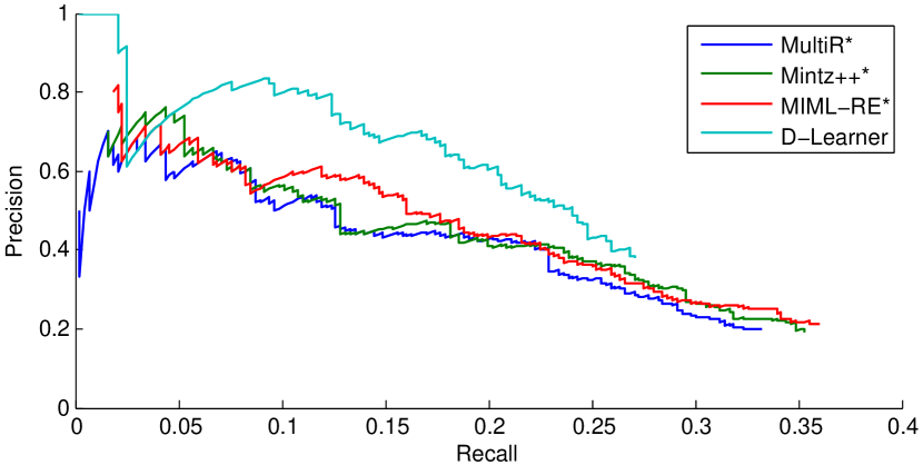
((a)) Disease domain.

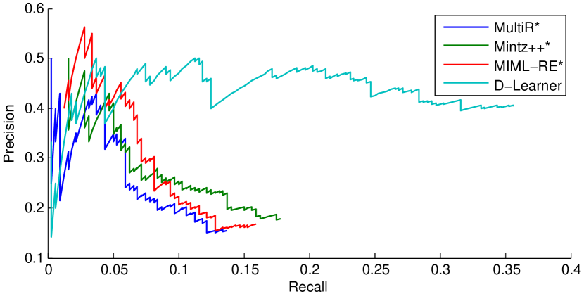
((b)) Drug domain.

Figure 3: Precision-recall curves.

D-Learner outperforms all the other systems. Compared with MultiR, Mintz++, and MIML-RE, the relative improvements under F1 are 19% to 27% in the disease domain, and 112% to 159% in the drug domain. This result shows that our D-Learner framework has overall superiority on the relation extraction task, mainly because of its capability of specifying these tailor-made constraints. The precision values of D-Learner are much higher than all compared systems on both domains. For recall, D-Learner performs much better than MultiR, Mintz++, and MIML-RE on the drug domain, and not as good as them on the disease domain.

The SVM-based baselines outperform the ProPPR-based baselines, which shows that the good performance of D-Learner on this task is not because of using ProPPR for its implementation. Comparisons between DS-X and DS-Dist-X show that the distillation step is useful for better results.

Precision-recall curves are given in Figures 3(a) and 3(b). For the disease domain, D-Learner’s precision is almost always better, at the same recall level, than any of the other methods. For the drug domain, D-Learner’s precision is generally better after the recall level 0.05.

4.4.5 Tuning with Bayesian Optimization

As listed in Table 5, we have 10 parameters: the number of training relation examples (#R), picked from the top of the ranked (by LP-based distillation) distantly labeled examples; the number of general negative relation examples (#NR); the numbers of type examples (#T) and general negative type examples (#NT); the example numbers of coFailure (#cF), mutexFailureR (#mFR), mutexFailureT (#mFT), docFailure (#dF), titleFailure (#tF), and sentFailure (#sF). The unlabeled constraint examples are randomly picked from the entire testing corpus. The 2nd and the 5th columns give the value ranges, and the 3rd and 6th columns give the step sizes while searching the optimal. Ten pages are annotated as the tuning data. We optimize the performance of D-Learner under F1, and the obtained optimal parameters are given in the 4th and 7th columns.

For both domains, D-Learner achieves better results by using a portion of top-ranked relation examples as training data. (This observation is consistent with the comparisons of DS-Dist-ProPPR vs. DS-ProPPR, and DS-Dist-SVM vs. DS-SVM.) It shows that using a smaller but cleaner set of training examples, combined with some SSL constraints and cotraining, can improve the performance.

For the disease domain, D-Learner performs better without cotraining type classifiers, thus, the optimal type related parameters, i.e. #T, #NT, #cF, and #mFT, for disease are 0. While for the drug domain, cotraining can bootstrap the performance of relation extraction. One explanation is that for a domain, e.g. drug, in which the second argument values of relations are less ambiguous (e.g. symptom entity for “sideEffect”), the cotrained type classifiers are accurate so that they can help the relation classifier learner explore useful features that are not captured by relation training examples. For the disease domain, the second argument values of relations have more ambiguity (e.g. “age” and “gender” for the relation “riskFactors”), which causes the learnt type classifiers inaccurate and unhelpful for the relation classifiers. With respect to the tailor-made constraints for relation extraction, i.e., docFailure, sentFailure, and titleFailure, D-Learner also behaves differently on the two domains. For the drug domain, it is optimal not using any examples from them, but for the disease domain, using all examples from them is preferred.

Table 5: Parameter tuning for relation extraction.

		Disease			Drug
	Range	Step	Optimal	Range	Step	Optimal
#R	(0, 5k]	10	2.1k	(0, 5k]	10	580
#NR	[0, 10k]	100	5.5k	[0, 10k]	100	1.2k
#T	[0, 10k]	200	0	[0, 10k]	200	10k
#NT	[0, 20k]	1k	0	[0, 20k]	1k	20k
#cF	[0, 100k]	10k	0	[0, 100k]	10k	100k
#mFR	[0, 20k]	2k	20k	[0, 20k]	2k	20k
#mFT	[0, 20k]	2k	0	[0, 20k]	2k	20k
#dF	[0, 30k]	2k	30k	[0, 20k]	2k	0
#sF	[0, 80k]	2k	80k	[0, 20k]	2k	0
#tF	[0, 30k]	2k	30k	[0, 20k]	2k	0

Note that the above conclusions on the effect of relation extraction constraints and cotraining type classifiers are under the integral setting of D-Learner, i.e. using both constraints and cotraining simultaneously. More tuning experiments show that for the drug domain, only using those relation extraction constraints also improves the performance, however, the improvement is not as significant as only using the cotraining setting; For the disease domain, only using the cotraining setting also improves the results, but not as much as only using those constraints. While using both constraints and cotraining in the integral setting, it does not necessarily end up with a value-added effect.

For both domains, the mutexFailure examples are found always helpful. Note that when $\textnormal{\#T}=0$, the mutexFailureT constraint becomes meaningless, thus, $\textnormal{\#mFT}=0$ for the disease domain. Another point to mention is that, as shown in Table 5, the optimal values of some parameters are the maximums in their ranges, which indicates that D-Learner is likely to achieve even better performance if more examples of these constraints are used.

5 Conclusions and Future Work

We proposed a general approach, D-Learner, to modeling SSL constraints. It can approximate traditional supervised learning and many natural SSL heuristics by declaratively specifying the desired behaviors of classifiers. With a Bayesian Optimization based tuning strategy, we can collectively evaluate the effectiveness of these constraints so as to obtain tailor-made SSL settings for individual problems. The efficacy of this approach is examined in two tasks, link-based text classification and relation extraction, and encouraging improvements are achieved. There are a few open questions to explore: adding hyperparameters (e.g., different weights for different constraints); adding more control over the supervised loss versus the constraint-based loss; and testing the approach on other tasks.

References

- Belkin et al. (2006) Mikhail Belkin, Partha Niyogi, and Vikas Sindhwani. Manifold regularization: A geometric framework for learning from labeled and unlabeled examples. The Journal of Machine Learning Research, 7:2399–2434, 2006.
- Bing et al. (2015) Lidong Bing, Sneha Chaudhari, Richard Wang C, and William W Cohen. Improving distant supervision for information extraction using label propagation through lists. In Proceedings of the 2015 Conference on Empirical Methods in Natural Language Processing, pages 524–529, Lisbon, Portugal, September 2015. Association for Computational Linguistics.
- Bing et al. (2016) Lidong Bing, Mingyang Ling, Richard C. Wang, and William W. Cohen. Distant IE by bootstrapping using lists and document structure. In Proceedings of the Thirtieth AAAI Conference on Artificial Intelligence, February 12-17, 2016, Phoenix, Arizona, USA., pages 2899–2905, 2016.
- Bing et al. (2017) Lidong Bing, Bhuwan Dhingra, Kathryn Mazaitis, Jong Hyuk Park, and William W. Cohen. Bootstrapping distantly supervised ie using joint learning and small well-structured corpora. In Proceedings of the Thirty First AAAI Conference on Artificial Intelligence, February 4-9, 2017, San Francisco, California, USA., 2017.
- Grandvalet and Bengio (2004) Yves Grandvalet and Yoshua Bengio. Semi-supervised learning by entropy minimization. In Advances in neural information processing systems, pages 529–536, 2004.
- Hoffmann et al. (2011) Raphael Hoffmann, Congle Zhang, Xiao Ling, Luke Zettlemoyer, and Daniel S Weld. Knowledge-based weak supervision for information extraction of overlapping relations. In Proceedings of the 49th Annual Meeting of the Association for Computational Linguistics: Human Language Technologies-Volume 1, pages 541–550. Association for Computational Linguistics, 2011.
- Joachims (1999) Thorsten Joachims. Transductive inference for text classification using support vector machines. In Proceedings of the Sixteenth International Conference on Machine Learning, ICML ’99, pages 200–209, San Francisco, CA, USA, 1999. Morgan Kaufmann Publishers Inc.
- Mintz et al. (2009) Mike Mintz, Steven Bills, Rion Snow, and Dan Jurafsky. Distant supervision for relation extraction without labeled data. In Proceedings of the Joint Conference of the 47th Annual Meeting of the ACL and the 4th International Joint Conference on Natural Language Processing of the AFNLP: Volume 2-Volume 2, pages 1003–1011. Association for Computational Linguistics, 2009.
- Riedel et al. (2010) Sebastian Riedel, Limin Yao, and Andrew McCallum. Modeling relations and their mentions without labeled text. In Machine Learning and Knowledge Discovery in Databases, pages 148–163. Springer, 2010.
- Sen et al. (2008) Prithviraj Sen, Galileo Mark Namata, Mustafa Bilgic, Lise Getoor, Brian Gallagher, and Tina Eliassi-Rad. Collective classification in network data. AI Magazine, 29(3):93–106, 2008.
- Snoek et al. (2012) Jasper Snoek, Hugo Larochelle, and Ryan P Adams. Practical bayesian optimization of machine learning algorithms. In F. Pereira, C. J. C. Burges, L. Bottou, and K. Q. Weinberger, editors, Advances in Neural Information Processing Systems 25, pages 2951–2959. Curran Associates, Inc., 2012.
- Surdeanu et al. (2012) Mihai Surdeanu, Julie Tibshirani, Ramesh Nallapati, and Christopher D. Manning. Multi-instance multi-label learning for relation extraction. In Proceedings of the 2012 Joint Conference on Empirical Methods in Natural Language Processing and Computational Natural Language Learning, EMNLP-CoNLL ’12, pages 455–465, Stroudsburg, PA, USA, 2012. Association for Computational Linguistics.
- Talukdar and Crammer (2009) Partha Pratim Talukdar and Koby Crammer. New regularized algorithms for transductive learning. In Machine Learning and Knowledge Discovery in Databases, pages 442–457. Springer, 2009.
- Wang et al. (2013) William Yang Wang, Kathryn Mazaitis, and William W Cohen. Programming with personalized pagerank: a locally groundable first-order probabilistic logic. In Proceedings of the 22nd ACM international conference on Conference on information & knowledge management, pages 2129–2138. ACM, 2013.
- Weston et al. (2012) Jason Weston, Frédéric Ratle, Hossein Mobahi, and Ronan Collobert. Deep learning via semi-supervised embedding. In Neural Networks: Tricks of the Trade - Second Edition, pages 639–655. 2012.
- Zhou et al. (2003) Dengyong Zhou, Olivier Bousquet, Thomas Navin Lal, Jason Weston, and Bernhard Schölkopf. Learning with local and global consistency. In Advances in Neural Information Processing Systems 16 [Neural Information Processing Systems, NIPS 2003, December 8-13, 2003, Vancouver and Whistler, British Columbia, Canada], pages 321–328, 2003.
- Zhu et al. (2003) X. Zhu, Z. Ghahramani, and J. Lafferty. Semi-supervised learning using Gaussian fields and harmonic functions. In Proceedings of ICML-03, the 20th International Conference on Machine Learning, 2003.
- Zhu (2005) Xiaojin Zhu. Semi-supervised learning literature survey. 2005.