Experimental simulation of quantum temporal steering beyond rotating-wave approximation

Abstract

Characterizing the dynamics of open systems usually starts with a perturbative theory and involves various approximations, such as the Born, Markov and rotating-wave approximation (RWA). However, the approximation approaches could introduce more or less incompleteness in describing the bath behaviors. Here, we consider a quantum channel, which is modeled by a qubit (a two-level system) interacting with a bosonic bath. Unlike the traditional works, we experimentally simulate the system-bath interaction without applying the Born, Markov, and rotating-wave approximations. To our knowledge, this is the first experimental simulation of the quantum channels without any approximations mentioned above, by using linear optical devices. The results are quite useful and interesting, which not only reveal the effect of the counter-rotating terms but also present a more accurate picture of the quantum channel dynamics. Besides, we experimentally investigate the dynamics of the quantum temporal steering (TS), i.e., a temporal analogue of Einstein-Podolsky-Rosen steering. The experimental and theoretical results are in good agreement and show that the counter-rotating terms significantly influence the TS dynamics. There are obviously different dynamics of TS in non-RWA and RWA channels. However, we emphasize that the results without RWA are closer to realistic situations and thus more reliable. Due to the close relationship between TS and the security of the quantum cryptographic protocols, our findings are expected to have useful applications in secure quantum communications and future interesting TS studies.

Department of Physics, Hangzhou Normal University, Hangzhou, Zhejiang 310036, China

State Key Laboratory of Precision Spectroscopy, Department of Physics, East China Normal University, Shanghai 200062, China

Department of Mathematics, Hangzhou Normal University, Hangzhou 310036, China
^⋆e-mail:sunzhe@hznu.edu.cn
^†e-mail:yangcp@hznu.edu.cn

Einstein-Podolsky-Rosen (EPR) steering is one of the most essential features in quantum mechanics. For a bipartite system in an entangled state, EPR steering problems refer to the quantum nonlocal correlations, which allow one of the subsystems to remotely prepare or steer the other one via local measurements. EPR steering is ususlly treated as an intermediate scenario lying in between the entanglement and the Bell nonlocality. As a result, some entangled states cannot be employed to achieve steering tasks, and some steerable states do not violate Bell-like inequalities [1, 2]. Recently, quantum steering problems have attracted considerable interest [3, 4, 5, 6, 7, 8, 9, 10, 11, 12, 13, 14, 15, 16, 17, 18, 19, 20, 21, 22]. Apart from the fundamental interests of steering in quantum mechanics [1, 2, 3, 4, 5, 6, 7, 8, 9, 10, 11, 12], there are lots of application motivations for EPR steering which is thought to be the driving power of quantum secure communication and teleportation [13, 14, 15]. For example, steering allows quantum key distribution (QKD) if one party trusts his own devices but not those of the other party [14]. An outstanding advantage is that this steering-dominated scenario is easier to implement, when compared with the completely-device-independent protocols [15].

Several inequalities in terms of sufficient conditions of steerability were employed to detect steerable states [1, 2, 3, 4], and such inequalities have been tested by several experiments [5, 6, 7, 8, 9]. Beyond inequalities, a number of possible measures were developed to quantify the quantum steerability [16, 17]. Very recently, Skrzypczyk et al. proposed a powerful measure named the steerable weight [18, 19]. Moreover, steerability was found to be equivalent to joint measurability [20, 21]. A close relationship between steerability and quantum-subchannel discrimination was discovered in [22].

Among the steering studies, a novel and important direction is to consider quantum steering in time, i.e., the so-called temporal steering (TS) [23]. Different from discussing the spatially-separated systems, TS problems focus on a single system at different times. In this frame, a system is sent to a distant receiver (say Bob) through a quantum channel, then a detector or manipulator (say Alice) performs some operations (including measurements on the system) before Bob receives the system and performs his measurement. The nonzero TS accounts for how strongly Alice’s choice of measurements at an initial time can influence the final state captured by Bob. In addition, TS also reveals a unique link between a quantum system’s past and future features. No third party can steer as strongly as Bob or gather full information about the final state. Based on this quantum origin, the TS inequality [23, 24, 25] becomes a very useful tool in verifying the suitability of a quantum channel for a certain QKD process. Compared with the spatial steering inequalities, TS inequality presents a superior applicability. Thus, the entanglement based scenarios are no longer necessary, and one can directly carry out the famous BB84 protocol and other related protocols [14, 23, 25, 26].

In order to quantify TS, a concept of temporal steerable weight was introduced in the literature [27], where the authors found that TS characterized by the weight can be used to define a sufficient and practical measure of strong non-Markovianity. This implies the evident dependence of TS dynamics on the properties of quantum channels. Moreover, it was found that TS is intrinsically associated with realism and joint measurability [28, 29].

In this paper, we investigate the influence of a quantum channel on the TS behavior. This is a particular TS problem rather than EPR steering, because the formation of the quantum correlation between the system’s initial and final state lies on the quantum channel. For example, during a unitary evolution, Alice is able to perfectly steer the final state received by Bob. A nontrivial case of TS refers to a non-unitary dynamics when Alice’s influence is erased partially or completely. Because TS is sensitive to the characteristics of the channel, a natural question arises: what kind of channel should we take into account?

Usually, the description of the dynamics of open systems starts with a perturbative theory and involves various approximations, such as the Born, Markov and rotating-wave approximation (RWA). However, it is widely believed that the approximation approaches introduce more or less the incompleteness of the description of the bath. An efficient numerical method that avoids using the above approximations was developed by Tanimura et al. [30, 31], who established a set of hierarchical equations that includes all orders of system-bath interactions. The hierarchy equation method has been successfully employed to describe the quantum dynamics of various physical and chemical systems [32, 33] as well as some quantum devices [34, 35].

The aims of this paper are as follows. Firstly, we propose a linear-optical setup to experimentally simulate a quantum channel modeled by a quantum two-level system (i.e., qubit) interacting with a bosonic bath, without applying Born, Markov and rotating-wave approximations. The experimental parameters accounting for the dynamics of the qubit are set by means of the hierarchy equation method. To the best of our knowledge, this is the first experimental simulation of this kind of quantum channel in a linear optical setup. Our experimental simulation offers a fruitful testbed for the studies of open quantum systems. Secondly, we experimentally investigate the TS problems in this channel. Our study indeed provides a more realistic representation of the environment influence than the usual quantum channels such as the amplitude damping channel, where the environment was only treated simply. Moreover, we found that there is a lack of experimental study of TS problems up to now. Some existing study [36] was only based on a phenomenologically-designed channel and thus it is impossible to highlight the important role of the system-bath interaction. In contrast, the channel under our study, governed by a system-bath Hamiltonian without RWA, allows us not only to reflect the special roles of the counter-rotating terms, but also to consider the system-bath couplings in arbitrarily strong regimes.

Results

System-bath model. We consider a qubit system interacting with a bosonic bath, described by a full Hamiltonian:

$$H=H_{\text{S}}+H_{\text{B}}+H_{\text{Int}},$$ (1)

where $H_{\text{S}}=\frac{\omega_{0}}{2}\sigma_{z}$ is the free Hamiltonian of the qubit (assuming $\hbar=1$), with $\sigma_{z}$ being the Pauli operator of the qubit and $\omega_{0}$ standing for the transition frequency between the two levels of the qubit; $H_{\text{B}}=\sum_{k}\omega_{k}b_{k}^{\dagger}b_{k}$ is the free Hamitonian of the bosonic bath with $b_{k}^{\dagger}$ and $b_{k}$ being the bosonic creation and annihilation operators of the $k$th mode of frequency $\omega_{k}$; and

$$H_{\text{Int}}=\sum_{k}\sigma_{x}\left(g_{k}b_{k}+g_{k}^{\ast}b_{k}^{\dagger}\right)$$ (2)

is the interaction Hamiltonian between the qubit and the bath with $g_{k}$ being the coupling strength between the qubit and the $k$th mode of the bath. One essential aspect of our study is that the interaction Hamiltonian $H_{\text{Int}}$ is in a non-RWA form. Because of the difficulty in studying this kind of non-RWA interaction, previous studies have used a RWA treatment for simplicity by assuming the interaction Hamiltonian as

$$H_{\text{Int}}^{\text{RWA}}=\sum_{k}\left(g_{k}\sigma_{+}b_{k}+g_{k}^{\ast}\sigma_{-}b_{k}^{\dagger}\right),$$ (3)

where the effect of the counter-rotating terms were omitted. Recently, it was found that the counter-rotating terms are necessary in order to accurately describe the spin-boson interaction [37] and using the conventional RWA approach may lead to faulty results [38].

Assume that the whole system is initially in the state $\rho_{\text{Tot}}\left(0\right)=\rho_{\text{S}}\left(0\right)\otimes\rho_{\text{B}}$, where $\rho_{\text{S}}\left(0\right)$ is the initial state of the qubit and chosen as a maximally mixed state $\rho_{\text{S}}\left(0\right)=\mathbb{I}/2$. The bath is considered to be initially in a vacuum state $\rho_{\text{B}}=|$vac$\rangle_{\text{BB}}\left\langle\text{vac}\right|,$ with $|$vac$\rangle_{\text{B}}\equiv\otimes_{k}|0\rangle_{k}$. The system-bath coupling spectrum is assumed as a Lorentz-type

$$J\left(\omega\right)=\frac{1}{2\pi}\frac{\gamma\lambda^{2}}{\left(\omega-\omega_{0}\right)^{2}+\lambda^{2}},$$ (4)

where $\lambda$ is the broadening width of the bosonic mode of frequency $\omega$, which is connected to the bath correlation time $\tau_{\text{B}}=\lambda^{-1}$. The relaxation time scale $\tau_{\text{S}}$, on which the state of the system changes, is related to $\gamma$ by $\tau_{\text{S}}=\gamma^{-1}.$ The $\gamma$ partly reflects the system-bath coupling strength, because one will obtain the effective coupling strength as $g_{\text{eff}}^{2}=\frac{1}{2}\gamma\lambda$ after integrating the spectrum $J\left(\omega\right)$ over the entire region of $\omega$.

The evolution under the total Hamiltonian (1) can be translated into the language of quantum channel. Thus the evolution map of the basis vectors can be described as

$$|g\rangle_{\text{S}}|\text{vac}\rangle_{\text{B}} \rightarrow \sqrt{p}|g\rangle_{\text{S}}|\text{even}\rangle_{\text{B},g}+\sqrt{1-p}|e\rangle_{\text{S}}|\text{odd}\rangle_{\text{B},g},$$

$$|e\rangle_{\text{S}}|\text{vac}\rangle_{\text{B}} \rightarrow \sqrt{q}|e\rangle_{\text{S}}|\text{even}\rangle_{\text{B},e}+\sqrt{1-q}|g\rangle_{\text{S}}|\text{odd}\rangle_{\text{B},e},$$

where $|g\rangle_{\text{S}}$ ($|e\rangle_{\text{S}}$) represents the ground (excited) state of the qubit while the vector $|$even$\rangle_{\text{B},i}$ ($|$odd$\rangle_{\text{B},i}$) describes the evolved vector of the bath, which is actually a superposition of all the number states (e.g., $\otimes_{k}|n_{k}\rangle_{k}$) with an even (odd) excitation number (i.e., $\sum_{k}n_{k}$ is even or odd). Note that the subscript $i\,$($=e,\,g$) of $|$even$\rangle_{\text{B},i}$ ($|$odd$\rangle_{\text{B},i}$) corresponds to the initial vector $|i\rangle_{\text{S}}|$vac$\rangle_{\text{B}}$. The vectors satisfy the orthogonality ${}_{\text{B},i}\langle$even$|$odd$\rangle_{\text{B},j}=0$ (including $i=j$ and $i\neq j$). They also satisfy the normalizing condition ${}_{\text{B},i}\langle$even$|$even$\rangle_{\text{B},i}=1$ and ${}_{\text{B},i}\langle$odd$|$odd$\rangle_{\text{B},i}=1$. The overlap ${}_{\text{B},i}\langle$even$|$even$\rangle_{\text{B},j}$ or ${}_{\text{B},i}\langle$odd$|$odd$\rangle_{\text{B},j}$ ($i\neq j$) outputs a complex number. The probabilities $p$ and $q$ are time-dependent, with $p\left(t\right)\in[0,1]$ and $q\left(t\right)\in[0,1]$. Then the reduced density matrix of the qubit becomes

$$\rho_{\text{S}}(t)=\left[\begin{array}[]{cc}\rho_{11}\left(t\right)&\rho_{12}\left(t\right)\\ \rho_{12}^{\ast}\left(t\right)&\rho_{22}\left(t\right)\end{array}\right],$$ (6)

where $\rho_{11}\left(t\right)=q\rho_{11}\left(0\right)+(1-p)\rho_{22}\left(0\right)$, $\rho_{22}\left(t\right)=(1-q)\rho_{11}\left(0\right)+p\rho_{22}\left(0\right)$, and $\rho_{12}\left(t\right)=\rho_{12}\left(0\right)\sqrt{pq}Z_{1}\left(t\right)+\rho_{21}\left(0\right)\sqrt{(1-q)(1-p)}Z_{2}\left(t\right)$. Here $\rho_{i,j}\left(0\right)$ ($i,j=1,2$) stands for the matrix elements of the qubit’s initial state, while $Z_{1}\left(t\right)\equiv$ ${}_{\text{B},g}\langle$even$|$even$\rangle_{\text{B},e}$ and $Z_{2}\left(t\right)\equiv$ ${}_{\text{B},e}\langle$odd$|$odd$\rangle_{\text{B},g}$ are the time-dependent complex numbers.

Experimental setup and implementation of the non-RWA channel. Our experimental setup is sketched in Fig. 1. In Fig. 1(a), pairs of photons with a 810 nm wavelength are produced by pumping a type-I beta-barium-borate (BBO) crystal with ultraviolet pulses at $405$ nm centered wavelength. Then one photon is led into a state-preparation process. That is, the first polarized beam splitter (PBS₁) selects the horizontally-polarized state $|H\rangle$ of the photon, and then a half wave plate (HWP) and a quarter-wave plate (QWP) can rotate $|H\rangle$ into one of the six eigenstates of the Pauli operators.

Fig. 1(b) accomplishes the task of the non-RWA quantum channel. We use the horizontal and vertical polarization modes $|H\rangle$ and $|V\rangle$ to encode the qubit’s basis states. The bath acts by a collective performance of four path modes $|i\rangle_{\text{p}},$ with $i\in\{0,1,2,3\}$. In order to briefly introduce the implementation of the channel, let us start from the output of PBS₂, where the $H$ and $V$ components are spatially separated so that each one can be rotated with the wave plate HWP₁ by angle $\theta_{1}\in[0,\pi/4]$ and the wave plate HWP₂ by angle $\theta_{2}$ $\in[0,\pi/4]$. After rotating by the wave plate HWP₁, the $|H\rangle$ mode becomes a superposition as $|H\rangle\rightarrow\cos 2\theta_{1}|H\rangle+\sin 2\theta_{1}|V\rangle$. By transmitting it along a loop, the superposition state undergoes PBS₂ again and couples with the spatial modes $|0\rangle_{\text{p}}$ and $|1\rangle_{\text{p}}$ encoded as the path numbers in Fig. 1(b), resulting in the state $\cos 2\theta_{1}|H\rangle|0\rangle_{\text{p}}+\sin 2\theta_{1}|V\rangle|1\rangle_{\text{p}}$.

It is worth noting that we make use of two Soleil-Babinet compensators (SBC₁ and SBC₂) in order to append a phase $\phi_{i}=\nu\tau_{i}$ to the passing components $H$ ($V$). Here, $\nu$ is the photon frequency and $\tau_{i}=L_{k}n_{l}/c$ is the traveling time of the photon across the SBC, where $L_{k}$ ($k=1,2$) denotes the thickness of SBC_1,2, $n_{l}$ ($l=H,V$) indicates the indices of refraction (corresponding to the $H$ and $V$ polarizations), and $c$ is the vacuum speed of light. Hence there are four phases $\phi_{1,2,3,4}\in[0,2\pi]$ appended to the polarization states of photons passing SBC₁ and SBC₂. This innovative design enables us to realistically describe the varying phase of the off-diagonal elements of the system’s density matrix.

In Fig. 1(b), there are several birefringent calcite beam displacers (BD_1,2,3,4) which deviate the $H$ component and transmit the $V$ one. Among them, we insert some wave plates to implement operations on the polarization states. The angles of HWP_3,4 are adjusted as $\theta_{3}\in[0,\pi/4]$ and $\theta_{4}\in[0,\pi/4]$ to transform a single component ($H$ or $V$) into a superposition form, while the angles of HWP_5,6,7,8 are fixed at $\theta_{5,6,7,8}=\pi/4$ to convert $H$ into $V$ or vice versa. The input-output states of Fig. 1(b) are mapped as follows(see details in the method section):

$$|H\rangle|0\rangle_{\text{p}} \rightarrow \cos 2\theta_{1}e^{i\phi_{1}}|H\rangle|0\rangle_{\text{p}}+\sin 2\theta_{1}e^{i\phi_{2}}|V\rangle\left|\Psi\right\rangle_{1,3},$$

$$|V\rangle|0\rangle_{\text{p}} \rightarrow \cos 2\theta_{2}e^{i\phi_{3}}|V\rangle\left|\Psi\right\rangle_{0,2}-\sin 2\theta_{2}e^{i\phi_{4}}|H\rangle|3\rangle_{\text{p}},$$

where $\left|\Psi\right\rangle_{1,3}\equiv\cos 2\theta_{3}|1\rangle_{\text{p}}-\sin 2\theta_{3}|3\rangle_{\text{p}}$ and $\left|\Psi\right\rangle_{0,2}\equiv\cos 2\theta_{4}|2\rangle_{\text{p}}-\sin 2\theta_{4}|0\rangle_{\text{p}}$. By comparing Eq. (LABEL:HV_map) with Eq. (LABEL:nonRWA_map), it can be seen that the reduced density operator of the system in Eq. (6) is successfully reproduced, by setting the parameters $q=\cos^{2}2\theta_{1}$, $p=\cos^{2}2\theta_{2}$, $Z_{1}=\sin\left(2\theta_{4}\right)e^{i(\phi_{3}-\phi_{1})}$, and $Z_{2}=\sin\left(2\theta_{3}\right)e^{i(\phi_{2}-\phi_{4})}$. It is noted that according to the hierarchy equation method [30, 34], the qubit state at an arbitrary time $t$ can be simulated by adjusting the parameters $\theta_{i}$ and $\phi_{i}$ according to the theoretical results obtained by the hierarchy equation method.

In Fig. 1(c), the density matrix of the output state is reconstructed by quantum tomography process where ten different coincidence measurement bases are set by QWPs, HWPs and PBSs. Eight of the bases are set along paths 0 and 3, while the rest are set along the paths 1 and 2. Finally, the photons are detected by single-photon detectors equipped with 10 nm interference filters.

As an application, our proposed experimental setup (Fig. 1) can be used to implement the channel governed by the RWA treatment of the interaction Hamiltonian in Eq. (3). Based on the evolution map in Eq. (LABEL:HV_map), one can set the HWP angles $\theta_{1}=0$, $\theta_{4}=\pi/4$, and adjust $\theta_{2}\in[0,\pi/4]$ according to the theoretical results with RWA. Furthermore, the phases $\phi_{1,3}$ is adjusted in $[0,2\pi]$ according to the theoretical results, and $\phi_{2,4}$ is set randomly. Then the evolution map in the Schrödinger picture reads:

$$~{}|H\rangle|0\rangle_{\text{p}}\rightarrow e^{i\phi_{1}}|H\rangle|0\rangle_{\text{p}},$$

$$~{}|V\rangle|0\rangle_{\text{p}}\rightarrow\sqrt{P_{\text{AD}}}e^{i\phi_{3}}|V\rangle|0\rangle_{\text{p}}+\sqrt{1-P_{\text{AD}}}e^{i\phi_{4}}|H\rangle|3\rangle_{\text{p}},$$

(8)

where $P_{\text{AD}}=\cos^{2}(2\theta_{2})$, and the spacial modes $|0\rangle_{\text{p}}$ and $|3\rangle_{\text{p}}$ correspond to the paths $0$ and $3$ in Fig. 1(b), respectively. If we further set the phases $\phi_{1,3,4}=0$ according to the interaction picture, Eq. (8) describes the so-called amplitude decay channel which is just the channel implemented in Ref. [39, 40]. The authors in [39] tested strong coupling cases in order to explore abundant non-Markovianity. However, it was theoretically predicated that the channels with or without RWA can cause quite different non-Markovian behavior especially in strong-coupling cases [41]. From this point of view, considering the quantum channels without RWA is of importance and an interesting question.

Another well-known channel, the so-called phase damping channel considered in [40], is also easy to implement in our scheme. Based on Eq. (LABEL:HV_map), by setting $\theta_{1,2}=0$, $\phi_{1,2,3,4}=0$ and adjusting $\theta_{4}\in[0,\pi/4]$, one can have the following evolution map:

$$~{}|H\rangle|0\rangle_{\text{p}}\rightarrow|H\rangle|0\rangle_{\text{p}},$$

$$~{}|V\rangle|0\rangle_{\text{p}}\rightarrow\sqrt{P_{\text{PD}}}|V\rangle|0\rangle_{\text{p}}-\sqrt{1-P_{\text{PD}}}|V\rangle|2\rangle_{\text{p}},$$ (9)

where $P_{\text{PD}}=\sin^{2}(2\theta_{4})$, and the spacial modes $|0\rangle_{\text{p}}$ and $|2\rangle_{\text{p}}$ correspond to the paths $0$ and $2$ in Fig. 1(b), respectively.

TS parameter. In the TS problem, a system is sent to a distant receiver (say Bob) through a quantum channel. Before Bob receives the system, a detector or manipulator (say Alice) performs some measurements on the system. Then the TS problem refers to the characterization of the influence of Alice’s measurement at an initial time $t_{A}$ (let $t_{A}=0$ in this paper) on the final state captured by Bob at a later time $t_{B}$. The TS in the qubit systems can be detected by a concept named as TS parameter $S_{N},$ which is defined in terms of a temporal analogue of the steering inequality [23, 25],

$$S_{N}\equiv\sum\limits_{i=1}^{N}E\left(\left\langle B_{i,t_{B}}\right\rangle_{A_{i,t_{A}}}^{2}\right)\leq 1,$$ (10)

where $A_{i,t_{A}}$ ($B_{i,t_{B}}$) stands for the $i$th observable measured by Alice (Bob) at $t_{A}$ ($t_{B}$) and the number of observable is $N=2$ or $3$.

$$E\left(\left\langle B_{i,t_{B}}\right\rangle_{A_{i,t_{A}}}^{2}\right)\equiv\sum\limits_{a=\pm 1}P\left(a|A_{i,t_{A}}\right)\left\langle B_{i,t_{B}}\right\rangle_{A_{i,t_{A}}=a}^{2},$$ (11)

with $P\left(a|A_{i,t_{A}}\right)$ being the probability of Alice’s measurement outcome $a=+1$ or $-1$. The Bob’s expectation value, conditioned on Alice’s measurement outcome, is defined as

$$\left\langle B_{i,t_{B}}\right\rangle_{A_{i,t_{A}}=a}\equiv\sum\limits_{b=\pm 1}bP\left(B_{i,t_{B}}=b|A_{i,t_{A}}=a\right),$$ (12)

where $P\left(B_{i,t_{B}}=b|A_{i,t_{A}}=a\right)$ denotes the condition probability of Bob’s measurement outcome $b$ (at $t_{B}$) on the evolved state starting from the collapsed version after Alice’s measurement with the outcome $a$ (at $t_{A}$). In this paper, we take the case of $N=2$ into account. The violation of the inequality in Eq. (10), i.e. $S_{2}>1$, is a sufficient condition for the steerability. Therefore, during an evolution, one can define the steerable durations conditioned by $S_{2}>1$.

Experimental and numerical results of TS parameter. We consider that Alice chooses a pair of the Pauli operators $\left\{\sigma_{i\text{ }},\sigma_{j}\right\}$ $(i,j=x,y,z)$ as the observables ($A_{i}$) measured on the initial state $\rho_{\text{S}}=\mathbb{I}/2$ of the qubit. After the measurement, the qubit state collapses to one of the six eigenstates of the Pauli operators with a probability $P\left(a|A_{i,t_{A}}\right)=1/2$. This process is usually difficult to implement in experiments, since it requires a set of nondestructive measurements. An equivalent way, adopted in this experiment, is to assume that Alice prepares qubit states by rotating the polarization mode $\left|H\right\rangle$ into one of the six eigenstates of the Pauli operators, and correspondingly multiplies a probability of $P\left(a|A_{i,t_{A}}\right)$. This preparation is completed by sequentially using the PBS₁, a HWP, and a QWP [see Fig. 1(a)]. Then the qubit in the prepared state is sent through the quantum channel [simulated in Fig. 1(b)] to Bob, who performs tomography measurements [Fig. 1(c)]. Therefore, Bob obtains the condition probabilities $P\left(B_{i,t_{B}}=b|A_{i,t_{A}}=a\right)$ and calculates $S_{2}$. Theoretically speaking, $S_{2}$ is a function of the time $t$, the channel parameter $\gamma$, and the parameter $\lambda$. Actually, in our experiment, the dynamics of $S_{2}$ is simulated by adjusting the angles of HWPs and the thicknesses of SBCs. The experimental errors are estimated from the statistical variation of photon counts, which satisfy the Poisson distribution.

Figure 2 shows $S_{2}$ vs evolution time scaled by $\omega_{0}$. In Fig. 2(a) and Fig. 2(b), the measurement bases are $\left|+\right\rangle$ ($\left|-\right\rangle$) and $\left|0\right\rangle$ ($\left|1\right\rangle$), which correspond to the eigenstates of $\sigma_{x\text{ }}$and $\sigma_{z}$, respectively. Our experimental and theoretical results are in good agreement and show the oscillation of TS parameter $S_{2}$ with time. More important is the steering limit, i.e., $S_{2}=1$, which is marked by a red-dashed horizontal line in Fig. 2. Above this limit, steerability is valid. The vertical dashed lines highlight the steerable durations corresponding to $S_{2}>1$. For the sake of comparison, we study two kinds of channels, i.e., the non-RWA channel and the RWA channel. The former is modeled by the Hamiltonian (2) and experimentally simulated according to the evolution map in Eq. (LABEL:HV_map), while the latter is modeled by the Hamiltonian (3) and experimentally simulated based on the evolution map in Eq. (8). In both of the cases of RWA and non-RWA channels, $S_{2}$ is suppresed below the steering limit in most of the evolution periods due to the quantum decoherence effects. However, the difference between the two cases is obvious. There are more peaks of $S_{2}$ over the steering limit in the RWA case [Fig. 2(b)] than the non-RWA case [Fig. 2(a)], which implies that the RWA channel appears to provide longer steerable durations. Similar conclusions can be made by comparing the results in Fig. 2(c) and Fig. 2(d), where another set of measurement bases are chosen, i.e., $\left|+\right\rangle$ ($\left|-\right\rangle$) and $\left|R\right\rangle$ ($\left|L\right\rangle$) (eigenstates of $\sigma_{x}$ and $\sigma_{y}$, respectively). However we should point out that the extra steerable durations in RWA cases are inauthentic, due to the essential defects in characterizing the system-bath interaction by using RWA.

Experimental and numerical results of TS weight. We also experimentally test the steerable weight of TS, i.e., $W_{\text{TS}}$ (see the definition in the method section), as illustrated in Fig. 3. The experimental implementations in the input-state preparation (at Alice’s side) and the tomography measurement on the output states (at Bob’s side) are the same as those in Fig. 2. The non-RWA case [Fig. 3(a)] and RWA case [Fig. 3(b)] are investigated. The parameters $\gamma$ and $\lambda$ are chosen as same as those in Fig. 2. Consequently, we compare the results shown in Figs. 3(a) and (b) with those in Figs. 2(c) and (d). Since $W_{\text{TS}}$ is defined according to the sufficient and necessary condition of the exsitence of TS, the data of $W_{\text{TS}}$ precisely tells us when the TS exists and disappears, especially for the durations below the TS limit $S_{2}=1$ [Fig. 2(c) and (d)], where the criterion $S_{2}$ is disabled to detect TS.

By comparison of Fig. 3(a) with Fig. 3(b), more interesting phenomena are found, i.e., there are obvious “sudden death” and “revival” of TS in the non-RWA channel, whereas they never appear in the RWA channel where TS tends to zero asymptotically. We shall emphasize that the quantum correlation like TS inevitably undergoes a sudden change to zero rather than a gradual decrease, especially when the characterization of the system-bath interaction becomes close to the actual situation. This also reminds us of the previous famous report on the sudden death of entanglement [42].

Discussion

With the proposed setup, we have experimentally implemented a non-RWA quantum channel and simulated the dynamics of a qubit system interacting with a bosonic bath, without applying Born, Markov and rotating-wave approximations. This kind of quantum channel provides a more realistic description of the environmental impact and allows a variety of investigation on coherence dynamics in open systems. Based on this channel, we have studied the important TS problem experimentally, which is attracting much attention recently. By means of the TS inequality, the experimental data agree well with the theoretical results, showing that quantum decoherence can significantly shorten the steerable durations. Furthermore, our investigation shows that although the RWA channel seems to provide longer steerable durations than the non-RWA case, the results without RWA are closer to realistic situations and thus more reliable.

By investigating the TS weight, we observed some new interesting phenomena in the non-RWA channel, i.e., the “sudden death” and “revival” of the TS, which however do not appear in the RWA channel. The RWA channel presents a false superiority compared with the non-RWA case.

Characterizing the quantum channel as precisely as possible is necessary and important in the study of quantum steering dynamics. Our studies show that an often-used approximation method such as the RWA leads to a deviation from the facts. It remains an open question to test other quantum correlation dynamics in the non-RWA quantum channel. On the other hand, since quantum steering inequalities are closely linked with the security of the quantum cryptographic protocols, our findings are expected to have valuable applications in secure quantum communications.

Methods

Implementation of the evolution map in Eq. (LABEL:HV_map). The input-output states for the setup in Fig. 1(b) are shown as follows:

$$|H\rangle \overset{\text{PBS}_{2},\text{HWP}_{1}}{\longrightarrow} \cos 2\theta_{1}|H\rangle|2\rangle+\sin 2\theta_{1}|V\rangle|1\rangle\overset{\text{SBC}_{1,2}}{\longrightarrow}\cos 2\theta_{1}e^{i\phi_{1}}|H\rangle|2\rangle+\sin 2\theta_{1}e^{i\phi_{2}}|V\rangle|1\rangle$$ (13)

$$\overset{\text{BD}_{1,2}}{\longrightarrow} \cos 2\theta_{1}e^{i\phi_{1}}|H\rangle|0\rangle+\sin 2\theta_{1}e^{i\phi_{2}}|V\rangle|1\rangle$$

$$\overset{\text{HWP}_{5,3}}{\longrightarrow} \cos 2\theta_{1}e^{i\phi_{1}}|V\rangle|0\rangle+\sin 2\theta_{1}e^{i\phi_{2}}(\cos 2\theta_{3}|V\rangle-\sin 2\theta_{3}|H\rangle)|1\rangle$$

$$\overset{\text{BD}_{3,4}}{\longrightarrow} \cos 2\theta_{1}e^{i\phi_{1}}|V\rangle|0\rangle+\sin 2\theta_{1}e^{i\phi_{2}}(\cos 2\theta_{3}|V\rangle|1\rangle-\sin 2\theta_{3}|H\rangle|3\rangle)$$

$$\overset{\text{HWP}_{7,8}}{\longrightarrow} \cos 2\theta_{1}e^{i\phi_{1}}|H\rangle|0\rangle+\sin 2\theta_{1}e^{i\phi_{2}}(\cos 2\theta_{3}|V\rangle|1\rangle-\sin 2\theta_{3}|V\rangle|3\rangle),~{}~{}~{}~{}~{}~{}~{}~{}~{}~{}$$

$$|V\rangle \overset{\text{PBS}_{2},\text{HWP}_{2}}{\longrightarrow} \cos 2\theta_{2}|V\rangle|2\rangle-\sin 2\theta_{2}|H\rangle|1\rangle\overset{\text{SBC}_{1,2}}{\longrightarrow}\cos 2\theta_{2}e^{i\phi_{3}}|V\rangle|2\rangle-\sin 2\theta_{2}e^{i\phi_{4}}|H\rangle|1\rangle$$ (14)

$$\overset{\text{BD}_{1,2}}{\longrightarrow} \cos 2\theta_{2}e^{i\phi_{3}}|V\rangle|2\rangle-\sin 2\theta_{2}e^{i\phi_{4}}|H\rangle|3\rangle$$

$$\overset{\text{HWP}_{6,4}}{\longrightarrow} \cos 2\theta_{2}e^{i\phi_{3}}(\cos 2\theta_{4}|V\rangle-\sin 2\theta_{4}|H\rangle)|2\rangle-\sin 2\theta_{2}e^{i\phi_{4}}|V\rangle|3\rangle$$

$$\overset{\text{BD}_{3,4}}{\longrightarrow} \cos 2\theta_{2}e^{i\phi_{3}}(\cos 2\theta_{4}|V\rangle|2\rangle-\sin 2\theta_{4}|H\rangle|0\rangle)-\sin 2\theta_{2}e^{i\phi_{4}}|V\rangle|3\rangle$$

$$\overset{\text{HWP}_{7,8}}{\longrightarrow} -\sin 2\theta_{2}e^{i\phi_{4}}|H\rangle|3\rangle+\cos 2\theta_{2}e^{i\phi_{3}}(\cos 2\theta_{4}|V\rangle|2\rangle-\sin 2\theta_{4}|V\rangle|0\rangle),~{}~{}~{}~{}~{}~{}~{}~{}~{}~{}\qquad$$

where the annotations above the arrows represent the devices through which the operations on the states are performed.

TS weight. Alice measures the observable $A_{i}$ on the system’s state at an initial time $t_{A}$, and gets the outcome $a$ with a probability of $P\left(a|A_{i,t_{A}}\right)$. Assume that there are $N$ observables, i.e. $A_{i}$ with $i=1,...,N$, and each of them is $m$ dimension (the case of $m=2$ is considered in this paper). After the measurement, the system’s state is mapped to $\rho_{a|A_{i}}$. Then, the system is sent to Bob through a quantum channel $\Lambda$. At time $t_{B}$, Bob receives the system and performs tomography measurements to obtain the state $\varsigma_{a|A_{i}}=\Lambda\left(\rho_{a|A_{i}}\right)$. In order to precisely quantify TS, a concept named TS weight, i.e. $W_{\text{TS}}$, is introduced via a semidefinite program as [19, 27]:

$$W_{\text{TS}}\equiv 1-\max\text{ Tr}\sum\limits_{\lambda}\varrho_{\lambda},$$ (15)

subject to

$$\tilde{\varsigma}_{a|A_{i}}-\sum\limits_{\lambda}D_{\lambda}\left(a|A_{i}\right)\varrho_{\lambda}\geq 0,\text{ \ }\forall a,A_{i},$$ (16)

and

$$\varrho_{\lambda}\geq 0,$$ (17)

where $\tilde{\varsigma}_{a|A_{i}}\equiv P\left(a|A_{i,t_{A}}\right)\varsigma_{a|A_{i}}$ stands for the un-normalized states received by Bob. The task of Bob is to check whether the states he receives can be written in a hidden-state form, i.e. $\sum_{\lambda}D_{\lambda}\left(a|A_{i}\right)\varrho_{\lambda}$ in Eq. (16), where $\lambda$ ($=1,...,m^{N}$) indicates a classical random variable. $\varrho_{\lambda}$ indicates a set of positive semidefinite matrices held by Bob, and $D_{\lambda}\left(a|A_{i}\right)$ is the deterministic single-party conditional probability according to Alice’s measurement outcome [19, 27]. Nonzero $W_{\text{TS}}$ implies that Bob cannot classically fabricate Alice’s measurement results, and thus the quantum temporal correlation (i.e., the TS) exists between Alice and Bob. Note that $W_{\text{TS}}$ comes from a sufficient and necessary characterization of steerability and quantifies the TS precisely.

References

Z.S. is supported by the National Natural Science Foundation of China under Grants No. 11375003, the Zhejiang Natural Science Foundation under Grant No. LY17A050003, the Program for HNUEYT under Grant No. 2011-01-011. C.P.Y is supported in part by the Ministry of Science and Technology of China under Grant No. 2016YFA0301802, the National Natural Science Foundation of China under Grant Nos. [11074062, 11374083]. Z.S., X.Q.X, J.S.J, and C.P.Y. are also supported by the Zhejiang Natural Science Foundation under Grant No. LZ13A040002 and the funds from Hangzhou City for the Hangzhou-City Quantum Information and Quantum Optics Innovation Research Team. The authors thank Prof. Chuan-Feng Li for valuable suggestions and Dr. Kai Sun and Dr. Xiaoming Hu for helpful discussions in the experimental implementation.

S.J.X. and Z.S. provided the idea. S.J.X., Y.Z., Z.S., and C.P.Y. designed the experiment. S.J.X., Y.Z., and Z.S. conducted the experiment and analyzed the data. Z.S., L.Y., X.Q.X., J.M.L., K.F.C., and C.P.Y. developed the theory. Z.S. and J.S.J. finished the numerical simulation. The manuscript was jointly written by the authors.

The authors declare no competing financial interests.

Figure 1: Experimental setup and the stages of the experiment. (a) The photon pairs with a 810 nm wavelength are produced via spontaneous parametric down-conversion. One of the two photons is used as the trigger for the coincident counts. The other photon is led to the preparation unit consisting of a polarized beam splitter (PBS₁), a half wave plate (HWP), and a quarter-wave plate (QWP). In the TS problems, this photon is prepared into one of the six eigenstates of the Pauli operators $\sigma_{x,y,z}$. (b) Simulation of the quantum channel without RWA in Eq. (LABEL:nonRWA_map). The angles of HWP_1,2,3,4 are adjusted in $[0,\pi/4]$, while the angles of HWP_5,6,7,8 are set at $\pi/4$. Two Soleil-Babinet compensators (SBC₁ and SBC₂) add relative phases to the passing components $H$ and $V$, respectively. The birefringent calcite beam displacers (BD_1,2,3,4) couple the polarization states $\left|H\right\rangle$ and $\left|V\right\rangle$ with the spacial modes $\left|i\right\rangle_{\text{p}}$ ($i=0,\,1,\,2,\,3$). (c) Quantum state tomography is implemented by two QWPs, four HWPs, and two PBSs. Finally, two single-photon detectors equipped with two 10 nm interference filters (IFs) are used for the photon counting.

Figure 2: TS parameter $S_{2}$ versus scaled time $\omega_{0}t$ in the non-RWA and RWA channels. (a) and (b) correspond to the measuring bases $|+\rangle~{}(|-\rangle)$ and $|0\rangle~{}(|1\rangle)$ which are the eigenstates of $\sigma_{x}$ and $\sigma_{z}$, respectively. While, (c) and (d) correspond to the measuring bases $|+\rangle~{}(|-\rangle)$ and $|R\rangle~{}(|L\rangle)$ which are the eigenstates of $\sigma_{x}$ and $\sigma_{y}$, respectively. The channel parameters, i.e., the system-bath coupling parameters $\gamma=2.5\omega_{0}$ and the broadening width of the bath mode $\lambda=0.05\omega_{0}$, which result in an effective strength of the system-bath coupling, i.e., $g_{\text{ eff}}=0.25\omega_{0}$. Horizontal red dashed lines indicate the steering limit. Vertical dashed lines point out the steerable durations corresponding to $S_{2}>1$. Inset: enlarged drawing with more data for the peaks of $S_{2}$ close to or beyond the steering limit.

Figure 3: TS weight vs scaled time $\omega_{0}t$ in the non-RWA and RWA channels. The measuring bases in (a) and (b) are $|+\rangle~{}(|-\rangle)$ and $|0\rangle~{}(|1\rangle)$ which are the eigenstates of $\sigma_{x}$ and $\sigma_{z}$, respectively. The values of parameters $\gamma$ and $\lambda$ are chosen as same as those in Fig. 2.

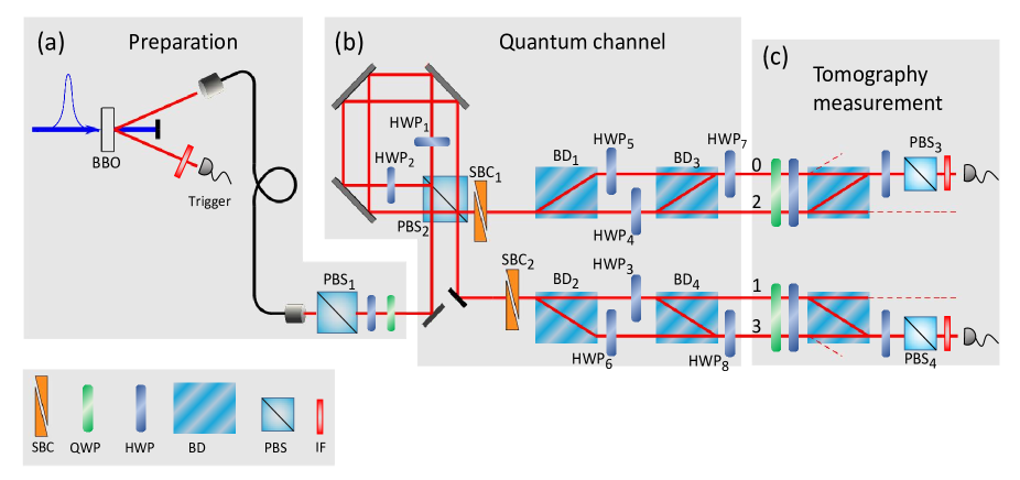
Figure 1:

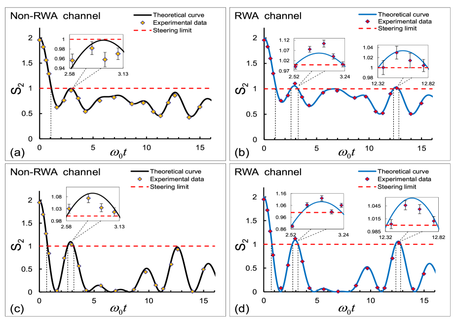
Figure 2:

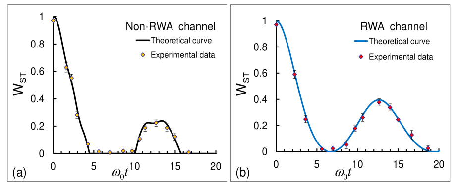
Figure 3:

References

- [1] Wiseman, H. M., Jones, S. J. Doherty, A. C. Steering, entanglement, nonlocality, and the Einstein-Podolsky-Rosen paradox. Phys. Rev. Lett. 98, 140402 (2007).
- [2] Jones, S. J., Wiseman, H. M. Doherty, A. C. Entanglement, Einstein-Podolsky-Rosen correlations, Bell nonlocality, and steering. Phys. Rev. A 76, 052116 (2007).
- [3] Marciniak, M., Rutkowski, A., Yin, Z., Horodecki, M. Horodecki, R. Unbounded Violation of Quantum Steering Inequalities. Phys. Rev. Lett. 115, 170401 (2015).
- [4] Zhu, H., Hayashi, M. Chen, L., Universal Steering Inequalities. Phys. Rev. Lett. 116, 070403 (2016).
- [5] Smith, D., Gillett, G., de Almeida, M., Branciard, C., Fedrizzi, A., Weinhold, T., Lita, A., Calkins, B., Gerrits, T., Wiseman, H., Nam, S. W. White, A. Conclusive quantum steering with superconducting transition edge sensors. Nat. Commun. 3, 625 (2012).
- [6] Kocsis, S., Hall, M. J. W., Bennet, A. J. Pryde, G. J. Experimental measurement-device-independent verification of quantum steering. Nat. Commun. 6, 5886 (2015).
- [7] Handchen, V., Eberle, T., Steinlechner, S., Samblowski, A., Franz, T., Werner, R. F. Schnabel, R. Observation of one-way Einstein-Podolsky-Rosen steering. Nat. Photon. 6, 596 (2012).
- [8] Sun, K., Ye, X. J., Xu, J. S., Xu, X. Y., Tang, J. S., Wu, Y. C., Chen, J. L., Li, C. F. Guo, G. C. Experimental Quantification of Asymmetric Einstein-Podolsky-Rosen Steering. Phys. Rev. Lett. 116, 160404 (2016).
- [9] Saunders, D. J., Jones, S. J., Wiseman, H. M., Pryde, G. J. Experimental EPR-steering using Bell-local states. Nat. Phys. 6, 845,849 (2010).
- [10] Armstrong, S., Wang, M., Teh, R. Y., Gong, Q. H., He, Q. Y., Janousek, J., Bachor, H. A., Reid, M. D. Lam, P. K. Multipartite Einstein-Podolsky-Rosen steering and genuine tripartite entanglement with optical networks. Nature Phys. 11, 167 (2015).
- [11] Bowles, J., Vértesi, T., Quintino, M. T. Brunner, N. One-way Einstein-Podolsky-Rosen steering. Phys. Rev. Lett. 112, 200402 (2014).
- [12] Walborn, S. P., Salles, A., Gomes, R. M., Toscano, F. Souto Ribeiro, P. H. Revealing Hidden Einstein-Podolsky-Rosen Nonlocality. Phys. Rev. Lett. 106, 130402 (2011).
- [13] He, Q. Y., Rosales-Zarate, L., Adesso, G. Reid, M. D. Secure Continuous Variable Teleportation and Einstein-Podolsky-Rosen Steering. Phys. Rev. Lett. 115, 180502 (2015).
- [14] Branciard, C., Cavalcanti, E. G., Walborn, S. P., Scarani, V. Wiseman, H. M. One-sided device-independent quantum key distribution: Security, feasibility, and the connection with steering. Phys. Rev. A 85, 010301(R) (2012).
- [15] Acin, A., Brunner, N., Gisin, N., Massar, S., Pironio, S. Scarani, V. Device-independent security of quantum cryptography against collective attacks. Phys. Rev. Lett. 98, 230501 (2007).
- [16] Jevtic, S., Pusey, M., Jennings, D. Rudolph, T. Quantum Steering Ellipsoids. Phys. Rev. Lett. 113, 020402 (2014).
- [17] Kogias, I., Lee, A. R., Ragy, S. Adesso, G. Quantification of Gaussian Quantum Steering. Phys. Rev. Lett. 114, 060403 (2015).
- [18] Pusey, M. F. Negativity and steering: A stronger Peres conjecture. Phys. Rev. A 88, 032313 (2013).
- [19] Skrzypczyk, P., Navascués, M. Cavalcanti, D. Quantifying Einstein-Podolsky-Rosen Steering. Phys. Rev. Lett. 112, 180404 (2014).
- [20] Quintino, M. T., Vértesi, T. Brunner, N. Joint Measurability, Einstein-Podolsky-Rosen Steering, and Bell Nonlocality. Phys. Rev. Lett. 113, 160402 (2014).
- [21] Uola, R., Moroder, T. Gühne, O. Joint Measurability of Generalized Measurements Implies Classicality. Phys. Rev. Lett. 113, 160403 (2014).
- [22] Piani, M. Watrous, J. Necessary and Sufficient Quantum Information Characterization of Einstein-Podolsky-Rosen Steering. Phys. Rev. Lett. 114, 060404 (2015).
- [23] Chen, Y. N., Li, C. M., Lambert, N., Chen, S. L., Ota, Y., Chen, G. Y. Nori, F. Temporal steering inequality. Phys. Rev. A 89, 032112 (2014).
- [24] Emary, C., Lambert, N. Nori, F. Leggett-Garg Inequalities, Rep. Prog. Phys. 77, 016001 (2014).
- [25] Bartkiewicz, K., Černoch, A., Lemr, K., Miranowicz, A. Nori, F. Temporal steering and security of quantum key distribution with mutually unbiased bases against individual attacks. Phys. Rev. A 93, 062345 (2016).
- [26] Tomamichel, M. Renner, R. Uncertainty Relation for Smooth Entropies. Phys. Rev. Lett. 106, 110506 (2011).
- [27] Chen, S. L., Lambert, N., Li, C. M., Miranowicz, A., Chen, Y. N. Nori, F. Quantifying non-markovianity with temporal steering, Phys. Rev. Lett. 116, 020503 (2016).
- [28] Li, C. M., Chen, Y. N., Lambert, N., Chiu, C. Y. Nori, F. Certifying single-system steering for quantum-information processing. Phys. Rev. A 92, 062310 (2015).
- [29] Karthik, H. S., Prabhu Tej, J., Usha Devi, A. R. Rajagopal, A. K. Joint measurability and temporal steering. J. Opt. Soc. Am. B 32, A34 (2015).
- [30] Tanaka, M. Tanimura, Y. Multistate electron transfer dynamics in the condensed phase: Exact calculations from the reduced hierarchy equations of motion approach. J. Chem. Phys. 132 214502 (2010).
- [31] Dijkstra, A. G. Tanimura, Y. Non-Markovian Entanglement Dynamics in the Presence of System-Bath Coherence. Phys. Rev. Lett. 104, 250401 (2010).
- [32] Ishizaki, A. Tanimura, Y. Dynamics of a Multimode System Coupled to Multiple Heat Baths Probed by Two-Dimensional Infrared Spectroscopy. J. Phys. Chem. A 111, 9269 (2007).
- [33] Jin, J. S., Zheng, X. Yan, Y. J. Exact dynamics of dissipative electronic systems and quantum transport: Hierarchical equations of motion approach. J. Chem. Phys. 128, 234703 (2008).
- [34] Ma, J., Sun, Z., Wang, X. Nori, F. Entanglement dynamics of two qubits in a common bath. Phys. Rev. A 85, 062323 (2012).
- [35] Sun, Z., Zhou, L. W., Xiao, G. Y., Poletti, D. Gong, J. B. Finite-time Landau-Zener processes and counterdiabatic driving in open systems: Beyond Born, Markov, and rotating-wave approximations. Phys. Rev. A 93, 012121 (2016).
- [36] Bartkiewicz, K., Černoch, A., Lemr, K., Miranowicz, A. Nori, F. Experimental temporal quantum steering. Sci. Rep. 6, 38076 (2016).
- [37] Albert, V. V. Quantum Rabi Model for N-State Atoms. Phys. Rev. Lett. 108, 180401 (2012).
- [38] Larson, J. Absence of Vacuum Induced Berry Phases without the Rotating Wave Approximation in Cavity QED. Phys. Rev. Lett. 108, 033601 (2012).
- [39] Fanchini, F. F., Karpat, G., Cakmak, B., Castelano, L. K., Aguilar, G. H., Jiménez Farías, O., Walborn, S. P., Souto Riberio, P. H. de Oliveira, M. C. Non-Markovianity through Accessible Information. Phys. Rev. Lett. 112, 210402 (2014).
- [40] Farí O. J., Aguilar, G.H., Valdés-Hernández, A., Ribeiro, P. H., Davidovich, L. Walborn, S.P. Observation of the emergence of multipartite entanglement between a bipartite system and its environment. Phys. Rev. Lett. 109, 150403 (2012).
- [41] Sun, Z., Liu, J., Ma, J. Wang, X. Quantum speed limits in open systems: Non-Markovian dynamics without rotating-wave approximation, Sci. Rep. 5, 8444 (2015).
- [42] Yu, T. Eberly, J. H. Finite-Time Disentanglement Via Spontaneous Emission. Phys. Rev. Lett. 93, 140404 (2004).