Increased persistence via asynchrony in oscillating ecological populations with long-range interaction

Abstract

Understanding the influence of structure of dispersal network on the species persistence and modeling a much realistic species dispersal in nature are two central issues in spatial ecology. A realistic dispersal structure which favors the persistence of interacting ecological systems has been studied in [Holland & Hastings, Nature, 456:792–795 (2008)], where it is shown that a randomization of the structure of dispersal network in a metapopulation model of prey and predator increases the species persistence via clustering, prolonged transient dynamics, and amplitudes of population fluctuations. In this paper, by contrast, we show that a deterministic network topology in a metapopulation can also favor asynchrony and prolonged transient dynamics if species dispersal obeys a long-range interaction governed by a distance-dependent power-law. To explore the effects of power-law coupling, we take a realistic ecological model, namely the Rosenzweig-MacArthur model in each patch (node) of the network of oscillators, and show that the coupled system is driven from synchrony to asynchrony with an increase in the power-law exponent. Moreover, to understand the relationship between species persistence and variations in power-law exponent, we compute correlation coefficient to characterize cluster formation, synchrony order parameter and median predator amplitude. We further show that smaller metapopulations with less number of patches are more vulnerable to extinction as compared to larger metapopulations with higher number of patches. We believe that the present work improves our understanding of the interconnection between the random network and deterministic network in theoretical ecology.

I Introduction

What determines the persistence of interacting spatially separated sub-populations? Or in other words, how long will these interacting sub-populations survive in a given time frame? This is indeed an important question in landscape ecology, where spatially separated sub-populations or patches of the same species create metapopulation structure via dispersal network Han98:Nature . Metapopulations are generally dynamic in nature ilmari2003long with frequent local extinctions, and dispersal within patches to allow recolonization, thereby preventing global extinction johst2002metapopulation . Metapopulation dynamics can be used to understand various ecological processes, including a variety of ecological and evolutionary dynamics that includes population size gyllenberg1992single , species persistence roy2005temporal , spatial distribution roy2008generalizing , epidemic spread mccallum2002disease , gene flow sultan2002metapopulation and local adaptation joshi2001local . It is necessary to understand the consequences of dispersal network structure because depending on it the metapopulation dynamics evolve hansson1991dispersal .

Dispersal is crucial for the survival of metapopulation as species that are connected through dispersal are less prone to extinction than that of disconnected ones holyoak1996persistence . On the contrary, there is a very high chance of global extinction if the patches are synchronized due to dispersal heino1997synchronous . Dispersal can be called a “double-edged sword” hudson1999moran because it can facilitates persistence at the local scale, but also leads to synchrony, and hence an increased probability of extinction. Therefore, there should be sufficient asynchrony in the patches to ensure species persistence hanski1995metapopulation ; ellner2001habitat . During asynchrony, as the species populations among the patches are different, so species can move from patches with higher abundance to connected patches thereby supporting the destination patches.

There has been a large number of studies including experimental dey2006stability ; ringsby2002asynchronous and theoretical holland2008strong on the ways to introduce asynchrony in metapopulation. Most significantly, Holland & Hastings holland2008strong have shown the role of dispersal network heterogeneity in species persistence by inducing asynchrony in the system. They have instigated asynchrony among the sub-populations by varying the network topology from regular to random and demonstrated that in general heterogeneous networks have longer periods of asynchronous dynamics, leading typically to lower amplitude fluctuations in population abundances.

The main question we address here is: Is there some other way to induce asynchrony and hence increased persistence in the system without using a heterogeneous network topology? Incorporating long-range interactions obeying distance-dependent power-law between the habitat patches we probe this question. In contrast to holland2008strong , here we have considered the role of distance between patches in the model with a regular network topology.

The motivation behind this is that in nature species are not likely to move to all the patches equally. Generally, species dispersal is dependent on the distance between habitat patches. Dispersal can be classified into “short-distance dispersal” (SDD) and “long-distance dispersal” (LDD). In nature, both SDD and LDD are prevalent with large intensity of short dispersals as compared to long dispersals. Long-distance dispersers greatly suffer from dispersal mortality as in a large ecological network not all the patches are likely to be accessible from a particular patch BoBe09:Oikos . Hence, the density of species moving to furthest patches decreases with increasing distance between patches, which can be seen in species like amphibians alex2005dispersal , butterflies baguette2003long , mites BoBe09:Oikos , etc. Although LDD events are typically rare, they are crucial to metapopulation survival bohrer2005effects ; trakhtenbrot2005importance .

Most metapopulation models consider only SDD while underestimating LDD hanski1999metapopulation ; baguette2003long . This leads to falsely estimating the scale of a metapopulation effect by reducing the extent of global dynamics to regional dynamics. Therefore, it is necessary to correctly incorporate LDD together with SDD into studies. One can incorporate both SDD and LDD into spatial ecological models by using distance-dependent power-law coupling. Previous empirical studies have shown that inverse power-law gave a better fit to empirical dispersal data hill1996effects ; thomas1997butterfly ; baguette2000population . Power-law dispersal is more general and universal coupling scheme which is motivated by many real-world systems. In the long-range coupling, each patch is connected to all the other patches with an effective dispersal strength according to power-law whose interaction strength is governed by an exponent (denoted by $s$). Studies have been performed using long-range interaction obeying power-law coupling in ferromagnetic spin models PhysRevB.54.R12661 , hydrodynamic interaction of active particles PhysRevLett.106.058104 ; C0SM01121E , ecological networks PhysRevE.94.032206 , biological networks PhysRevLett.74.3297 , etc. The power-law exponent $s$ represents how likely the species is to travel to a further habitat. A higher value of $s$ suggests that the likelihood of a species to travel to a further habitat is less as compared to a lower value of $s$.

Here we analyze an ecological network of habitat patches whose local dynamics are governed by the Rosenzweig-MacArthur model RoMa63 and the dispersal between the patches is governed by a long-range interaction obeying a distance-dependent power-law. The effective strength of long-range interaction between habitat patches decreases with increasing power-law exponent. In this paper, we show the dramatic transformation in the spatiotemporal dynamics when species are connected by power-law. We compute numerical measures like cluster distribution, interpatch synchrony, predator amplitude and transient time to understand species persistence. Our key finding is the asynchronicity that is generated, surprisingly, even in a regular network by incorporating power-law dispersal. Furthermore, by varying the network size we find that metapopulations with larger number of patches are more persistence (hence less prone to extinction) in comparison with metapopulations with less number of patches.

We organize the paper as follows: First, we discuss the structure of ecological network and the model used to govern the local dynamics, along with the coupling used to model dispersal dynamics between patches in Sec. II. Then, we present the effects of power-law on the spatiotemporal dynamics of the model in Sec. III by calculating several dynamical measures. Here, we also show the effect of network size in species persistence. Finally, in Sec. IV we discuss the importance of our findings.

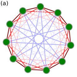
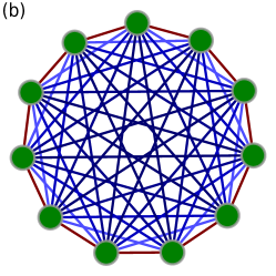
Figure 1: (Color online) All patches are connected to all patches in the network, and dispersal is bi-directional following the long-range interaction as modeled in Eq. (1). Color of the edges represents power-law strength ($r^{-s}$) between patches with: (a) $s=0.5$ and (b) $s=1.5$. Higher $s$ suggests that the species is less likely to move to further patches. Each spatially separated patches are marked with filled circles. Here we consider an ecological network with 11 patches.

II The Network Model

We consider an $n$-patch/node prey-predator system where uncoupled dynamics in each patch are governed by a non-dimensional form of the well known Rosenzweig-MacArthur model RoMa63 . A schematic picture of the ecological network is depicted in Fig. 1. In the network, we assume that dynamics within each patch are identical and the dispersal dynamics of prey-predator are modeled as follows:

$$\frac{dh_{i}}{dt} =h_{i}(1-\theta h_{i})-\frac{p_{i}h_{i}}{1+h_{i}}$$

$$\;\;\;\;+d_{h}\left(\frac{1}{\xi(s)}\sum_{r=1}^{m}\frac{h_{i-r}+h_{i+r}}{r^{s}}-h_{i}\right),$$ (1a)

$$\frac{dp_{i}}{dt} =\frac{\phi p_{i}h_{i}}{1+h_{i}}-\eta p_{i}+d_{p}\left(\frac{1}{\xi(s)}\sum_{r=1}^{m}\frac{p_{i-r}+p_{i+r}}{r^{s}}-p_{i}\right),$$ (1b)

where $i=1,2,\dots,n$ is the patch index, the prey and predator density are represented by $h_{i}$ and $p_{i}$, respectively for the $i$-th patch with all indices are taken modulo $n$ (the total number of patches in the network). The local (uncoupled) dynamics in each patch are governed by the following parameters: $\theta$ is the strength of prey self-regulation, $\phi$ is the predator conversion efficiency, and $\eta$ is the predator mortality rate. The spatial dynamics are governed by: dispersal rate $d_{h}\text{ and }d_{p}$ for prey and predator, respectively, the dispersal range $m$, and $\xi(s)=2\sum_{r=1}^{m}r^{-s}$ is the normalization constant. The interaction between the neighboring patches follows a dispersal rate whose intensity decays with the distance $r$ between patches as inverse power law $r^{-s}$. Here, $s\geq 0$ is the power-law strength PhysRevLett.74.3297 and $r$ $(r=1,\dots,m)$ is the distance between $i$-th and $j$-th patches, which is defined to be the minimum number of edges required to move from the $i$-th patch to the $j$-th patch along the arc with $m=(n-1)/2$ for odd number of patches.

The significance of this model (1) of ecological network with long-range coupling is that one can take into account both SDD and LDD along with their intensities. Also it is possible to control the effective LDD by varying the parameter $s$ only. For instance, when $s=0$, a species is equally likely to move into any patch resulting in the equal intensities of SDD and LDD, whereas when $s>0$, a species is less likely to move to a farther patch as compared to a nearby patch resulting in less intensity of LDD as compared to SDD. However, this form of connectivity is different from the usual ecological network models with a fixed dispersal rate holland2008strong ; GoHa08 ; GoHa11 ; hastings2001transient ; wall2013synchronization .

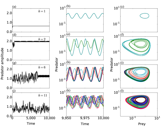
Figure 2: (Color online) Time series of ((a), (d), (g), (j)) total predator amplitude and ((b), (e), (h), (k)) predator species, and ((c), (f), (i), (l)) phase portrait of predator vs prey for different cluster solutions. Local dynamics are governed by strong prey self-regulation $\theta=0.3$ and predator mortality rate $\eta=1$ comparable to prey birth rates. Dispersal rates are: $d_{h}=2^{-5}$ and $d_{p}=2^{-6}$. Other parameters are: ((a), (b), (c)) $s=0,\phi=2,k=1$; ((d), (e), (f)) $s=0,\phi=3,k=2$; ((g), (h), (i)) $s=1,\phi=3,k=6$; and ((j), (k), (l)) $s=2,\phi=3,k=11$.

III Results

We explore the spatiotemporal dynamics of the coupled Rosenzweig-MacArthur model (1) with variations in the parameter $s$. We always fix the dispersal range to be $m=(n-1)/2$ (i.e., we consider a globally coupled network) and vary $s$. In other words, all the patches are accessible by a disperser from any patch, however the dispersal density between them will depend on the distance between the patches and hence on the value of $s$. Therefore, we start with a globally coupled network ($s=0$) and vary the $s$, effectively reducing the strength of long-range interactions.

Our main goal is to show that asynchrony can be introduced into the system by varying the power-law exponent $s$. We investigate the effect of $s$ on species persistence and calculate measures like cluster identification, parameter of synchrony, median predator amplitude and mean transient fraction to justify our key findings. We also study how predator dispersal $d_{p}$ and $\phi$ affect the results. Before we proceed, let us discuss the integration scheme we used to solve Eqs. (1). We perform the numerical integration using backward-differentiation formula method in CVODE cohen1996cvode ; holland2008strong . Prey initial conditions are independently and identically distributed, with $\log_{10}(h_{i}(0))$ uniformly distributed on the interval $(-5,1+\log_{10}\hat{h})$. Similarly, predator initial conditions are independently and identically distributed, with $\log_{10}(p_{i}(0))$ uniformly distributed on the interval $(-5,1+\log_{10}\hat{p})$, where, $\hat{h}=\frac{\eta}{\phi-\eta}$ and $\hat{p}=(1+\hat{h})(1-\theta\hat{h})$ holland2008strong .

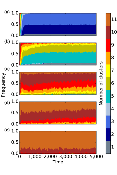
Figure 3: (Color online) Distribution of cluster states for different values of $s$: (a) $s=0$; (b) $s=0.3$; (c) $s=0.6$; (d) $s=0.9$; and (e) $s=1.2$. The local dynamics are governed by weak predation $(\phi=2.7)$, strong prey self-regulation $(\theta=0.3)$ and predator mortality rate $(\eta=1)$ comparable to prey birth rates. The spatial parameters are $d_{h}=2^{-5}$ and $d_{p}=2^{-6}$. Number of clusters increases with increasing values of $s$. The above results in each sub-figures correspond to $100$ numerical simulations carried out independently.

III.1 Cluster analysis

It is interesting to observe that Eqs. (1) can show a variety of spatial dynamics, ranging from global synchrony to global asynchrony. Cluster analysis is used to study the synchronous dynamics of the system. To compare the dynamics between a pair of patches $(i,j)$, linear correlation coefficient $\rho_{ij}$ of prey time series at time $t$ is calculated as follows:

$$\rho_{ij}=\frac{<h_{i}h_{j}>-<h_{i}><h_{j}>}{\sqrt{<h_{i}^{2}>-<h_{i}>^{2}}\sqrt{<h_{j}^{2}>-<h_{j}>^{2}}},$$

where, $<\dots>$ is average over the window $[t,t+4\overline{T}]$, with $\overline{T}$ as the mean period of a predator-prey cycle for a given simulation, averaged over all patches. We calculate the linear correlation coefficient $\rho_{ij}$ at each unit time.

Two patches would behave identically with time if they have $\rho_{ij}>0.999$. So, we segregate the patches into clusters and define a cluster to be a set of patches with $\rho_{ij}>0.999$. We call a $k$-cluster to be the maximum number of clusters. In this way, a $k$-cluster solution could be formed where the $n$ patches could be assigned to $k~{}(\leq n)$ clusters of patches with identical dynamics. We compute the frequency of $k$-cluster solution with time, where the frequency at time $t$ is defined as:

$$\mbox{Frequency of $k$-cluster solution}=\frac{\mbox{No. of $\leq k$-clusters }}{\mbox{No. of simulations}}$$

Apart from global synchrony (we may call one cluster solution) and global asynchrony (n-cluster solution), Eqs. (1) can result in intermediate solutions between two and ($n-1$)-clusters of synchronous patches with variations in $s$. These $k$-cluster solutions may vary over time thereby converging to a single $k$-cluster solution with higher asynchrony in the initial transient phase. We observe different kinds of cluster behaviors which can be clearly seen in Fig. 2. It is important to keep in mind that there might be several $k$-cluster solutions (c.f. Fig. 3) for $2\leq k\leq n$ even for same parameter values. This is due to the fact that the network being a higher dimensional system it has multiple steady states, thereby making it necessary to carry out a large ensemble of simulations with a collection of different initial conditions. Figure 3 shows the variation in solutions for different power-law exponent $s$. Surprisingly we see that the system is driven from synchrony to asynchrony by varying the long-range interaction through $s$ even with a regular network topology. We can say that the species is more persistent when $s$ is increased, as asynchronous patches are less prone to extinction than synchronous patches because synchronous patches are more vulnerable to environmental perturbation as minimum level of all sub-populations occur simultaneously at some time holyoak1996persistence . Asynchrony also results in rescue effect as the species can move from a patch with higher population to a patch with lower population thereby recolonizing the population.

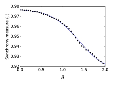
Figure 4: (Color online) Synchrony order parameter ($\sigma$) with variations in $s$. The other parameters are $d_{h}=2^{-10}$, $d_{p}=2^{-10}$, $\phi=2$, $\eta=1$, and $\theta=0.3$. Network size is 11. Points are fitted by a polynomial of degree 4 (blue curve). The synchrony order parameter ($\sigma$) decreases with increasing $s$. The above result corresponds to $100$ numerical simulations carried out independently.

III.2 Measure of interpatch synchrony

We also measure the amount of change in interpatch synchrony with variations in $s$ (see Fig. 4). To quantify the effect of change in long-range interaction in system dynamics, we apply a synchrony order parameter (denoted by $\sigma$) komin2011synchronization for a time period of 10000 and vary $s$, where:

$$\sigma=\sqrt{1-\Bigg{\langle}\frac{\sum_{i=1}^{n}[h_{i}(t)-\overline{h}(t)]^{2}}{\sum_{i=1}^{n}h_{i}(t)^{2}}\Bigg{\rangle}},$$

with $\overline{h}(t)=\frac{1}{n}\sum_{i=1}^{n}h_{i}(t)$ and $\Big{\langle}\dots\Big{\rangle}$ denotes the average over mentioned time. The value of the parameter $\sigma$ varies between 0 and 1. It is equal to 0 when there is no synchrony and 1 if the patches are perfectly synchronized. The value is in between 0 and 1 when the patches are partially synchronized. We find that with an increase in $s$, the synchrony order parameter decreases. As shown in Fig. 4, the interpatch synchrony decreases with increasing $s$ and hence species persistence increases as we increase $s$. We fit a curve with the synchrony parameter values $\sigma$ for visual guidance.

III.3 Total predator amplitude

As the species in a patch is oscillating with time there will be instances of time when the population would be at its minimum. The species would be at risk if the minimum densities occur at the same time instance for all the patches. However, the chances of extinction can be reduced if the minimum populations corresponding to different patches occur at considerably different time. In other words, we could say that a population would have higher extinction risk if the fluctuations are high. To quantify these fluctuations we calculate total predator amplitude, following holland2008strong which is defined as:

$$\mbox{Total predator amplitude}=\log_{10}\left(\frac{max(\sum_{i=1}^{n}p_{i})}{min(\sum_{i=1}^{n}p_{i})}\right),$$

over the window of interest $4\overline{T}$. The way the total predator amplitude is defined, we could say its value would be high when the populations are synchronized while the value would be low if the populations are asynchronous. Figures 2(a), (d), (g) and (j) shows the amplitude fluctuations with time for different parameter values. The amplitude fluctuations would depend on the number of clusters as higher number of clusters would correspond to lower total predator amplitude which can be clearly seen in Fig. 2.

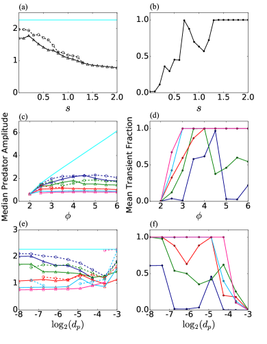
Figure 5: (Color online) Predator amplitude and transient duration: ((a), (c), (e)) Median total predator amplitude during transient (triangles, solid lines) and asymptotic (open circles, dashed lines) solution phases for a regular network; ((b), (d), (f)) mean transient fraction for different parameters. The cyan line in ((a), (c), (e)) corresponds to global synchronous solution for the chosen parameter values: ((a), (b)) $\phi=3.0,\eta=1,\theta=0.3,d_{h}=2^{-5},d_{p}=2^{-6}$; ((c), (d)) $\eta=1,\theta=0.3,d_{h}=2^{-5},d_{p}=2^{-6}$; and ((e), (f)) $\phi=3.0,\eta=1,\theta=0.3,d_{h}=2^{-5}$. The color coding’s are as follows: $s=0.0$ (dark blue); $s=0.5$ (green); $s=1.0$ (red); $s=1.5$ (light blue); and $s=2.0$ (pink). The above result corresponds to 150 numerical simulations carried out independently.

We divided the time series into two phases: transient and asymptotic phases, where transient phase is defined as the time before all the patches display constant or periodic phase evolution. The remaining time is defined to be the asymptotic phase. There are instances when the populations would have never reached the asymptotic phase for the given duration ($t=10000$). We used an automated algorithm as described in Ref. holland2008strong to estimate transient time from numerically integrated solutions of Eqs. (1).

The main idea behind dividing the time into two phases rather than only considering the asymptotic phase is because studies hastings2004transients ; hastings2001transient have shown the necessity to consider both of them. In most of the studies it is assumed that ecological systems that are observed in nature correspond in some way to stable equilibria hastings2004transients . This is not the case because for example, if we want to study the persistence of plankton species huisman1999biodiversity , the seasonality effectively reduces the relevant timescale to less than one year especially in temperate lakes, then we have to consider the model behavior within a singe season and then restart the model the next season, rather than looking at the long term result of the model. Also in the case of adaptive management of renewable resources, it is necessary to understand the short-term responses than the long-term outcomes hastings2004transients .

As we have divided time into two phases: transient and asymptotic, we separate the total predator amplitude into two time series and then we take the median of these time series which we call as median predator amplitude (MPA) for transient and asymptotic phases. Figure 5 depicts MPA and transient time for different parameters. It is important to note that here MPA is taken to be the average of 150 ensemble of simulations because different initial conditions might lead to different spatiotemporal dynamics. As MPA tells us how much the total population is fluctuating, so a higher MPA would correspond to a lower species persistence and vice versa. Figures. 5(a) and 5(b) represent variations in MPA and transient time respectively with $s$. Interestingly, near $s=0$ (i.e., when dispersal is independent of distance) we observe both transient and asymptotic MPA to have a higher amplitude closer to that of a global synchronous solution which has a high extinction risk because populations in all the patches have identical dynamics and any perturbation when the population is very low might lead to global extinction. This global extinction can be avoided if populations in all the patches do not behave exactly the same with time (i.e., they are asynchronous). Importantly, with increasing $s$, there is a decrease in amplitudes leading to higher species persistence. Surprisingly, MPA at transient phase is lower than MPA at asymptotic phase which suggests that the species have higher extinction risk during asymptotic phase than at the transient phase. The reason behind missing data point for MPA in asymptotic phase is that for higher values of $s$ the system never reaches asymptotic phase in 10000 units of time. For lower values of $s$, we see very low transient time in Fig. 5(b) and with increasing $s$, mean transient fraction saturates to 1. These higher transient time corresponds to asynchronous solutions with large number of clusters as also depicted in Fig. 3.

We also investigate the effect of predator efficiency $\phi$ on MPA and transient time. Therefore, we plotted MPA and transient time for different values of $s$ with respect to $\phi$ in Figs. 5(c) and 5(d). One can conclude that by varying predator efficiency, $\phi$, the system can be driven from low to high MPA. For higher predator efficiencies, the global synchronous solution has higher order of magnitudes thereby making global extinction very much likely. An important result is, for any value of $\phi$, MPA decreases and transient fraction increases or saturates to one with $s$ from which it can be concluded that the system is driven to higher persistence. However, for a very low value of $\phi$ (i.e., $\phi=2$), the system has globally synchronous solution for any value of $s$, thereby having a very high chance of global extinction. From Fig. 5, one might say that the system with higher values of $s$ spend much more time on lower-amplitude transient solutions.

Another important parameter to consider in this study is the predator dispersal rate $d_{p}$. Increasing the predator dispersal from a low value, the system moves from longer to shorter transients. For almost all dispersal rates in Figs. 5(e) and 5(f), the system moves from high to low MPA and shorter to longer transients when $s$ has increased. For $s=0$, there is almost no transient resulting in no transient MPA for some predator dispersal rate, as shown in Figs. 5(e) and 5(f). The transient fraction saturates to one for higher values of $s$. However, for high value of dispersal rate, we observe global synchronous solution irrespective of $s$.

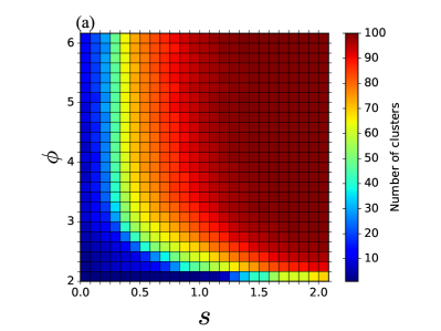
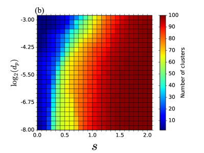
Figure 6: (Color online) Variation of cluster solutions with spatial and dispersal parameters: (a) Dispersal rates are $d_{h}=2^{-5}$ and $d_{p}=2^{-6})$ and (b) prey dispersal rate $d_{h}=2^{-5}$. Local dynamics are governed by weak predation $\phi=3.0$, strong prey self-regulation $\theta=0.3$ and predator mortality rate $\eta=1$. Each grid summarizes 120 numerical simulations carried out independently.

III.4 Combined effect of system parameters and $s$ in a large network

Until now we performed our study with an ecological network of 11 nodes. Here, we consider a relatively large network of 101 nodes and study their dynamics. In this case, we see a variety of $k$-cluster solutions varying from global synchrony ($k=1$) to global asynchrony ($k=101$). We varied the predator efficiency and predator dispersal rate and took the mean of $k$-cluster solutions at time $t=5000$ for 120 simulations. Figures 6(a) and 6(b) represent how the cluster solutions depend on a local parameter $\phi$ and a dispersal parameter $d_{p}$ for a large network of size 101 nodes. For a very low value of predator efficiency ($\phi=2$) in Fig. 6(a), we see the least number of clusters as compared to other values of $\phi$. Increasing the predator efficiency $\phi$ leads to higher number of clusters, however this is not true when $s$ is very low. With increasing $s$, the number of clusters increases thereby making the system asynchronous leading to higher persistence. Surprisingly, at $s=0$, the number of clusters is very low irrespective of $\phi$. This tells us that when dispersal is independent of distance, the rate of synchronization is very high and as a consequence it may lead to global extinction.

Figure 6(b) depicts how the average number of $k$-clusters vary with predator dispersal rate ($d_{p}$) and power-law exponent ($s$). Higher predator dispersal leads to lower number of $k$-clusters as compared to lower predator dispersal, which is also intuitive because higher dispersal leads to higher synchronization in sub-populations leading to less number of clusters. However, for higher values of $s$ (i.e., near $s=2$), the population is asynchronised, which is independent of the predator dispersal rate. At $s=0$, irrespective of the dispersal rates the number of clusters is very low from which we can infer that even in low dispersal rate the synchrony is very high when dispersal is independent of distance.

III.5 Effect of network size

Next, we study the influence of network size on the MPA and transient time. Figure 7 illustrates how the MPA and transient time vary with the network size for a particular $s$. It can be seen that the transient fraction increases and MPA during transient regime decreases with increase in the network size. For $s>0$, the transient fraction saturates to one as the network size increases. Remarkably, we find that with increasing network size the MPA decreases thereby suggesting that smaller networks have higher MPA and thus a lower species persistence.

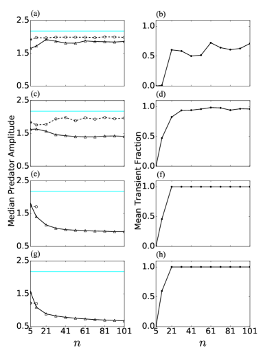
Figure 7: (Color online) Predator amplitude and transient duration as a function of network size. Median total predator amplitude during transient (triangles, solid lines) and asymptotic (open circles, dashed lines) solution phases for a regular network. The cyan line corresponds to global synchronous solution for the chosen parameter values: $\eta=1,\;\theta=0.3,\;d_{h}=2^{-5}$, and $d_{p}=2^{-6}$. (a,b) $\phi=3,\;s=0$; (c,d) $\phi=3,\;s=0.3$; (e,f) $\phi=3,\;s=0.5$; and (g,h) $\phi=3,\;s=1.0$. The above result corresponds to 150 numerical simulations carried out independently.

The motivation behind considering variable network size in our study is to understand the effect of metapopulation size in the dynamics of the considered ecological network HaMoGy96:Amnat . We find that small metapopulations (i.e., with less number of patches) further increases the risk of global extinction because smaller networks are much easier to synchronize as compared to larger networks. Since, a small network will have less number of $k$-cluster solution as compared to a large network. Hence, large metapopulations which are spread over large landscapes (with more spatially separated patches), more known areas and connectivities are less prone to extinction as they are difficult to synchronize and hence carries the characteristic of higher species persistence.

IV Discussions and Conclusions

Synchrony and stability are often considered as conflicting outcomes of dispersal briggs2004stabilizing . Stability here refers to the state when populations linked by dispersal are more persistent and hence less prone to extinction than the isolated ones. However, synchrony on the other hand can result in global extinction. In many studies it has been shown that heterogeneous network is required to generate stability and asynchrony simultaneously holland2008strong ; singh2004role ; loreau2003biodiversity ; briggs2004stabilizing . On the contrary, we use a regular network with power-law coupling to induce stability and asynchrony.

We have presented the importance of distance-dependent dispersal in the ecological dynamics. We have shown how the ecological dynamics vary when the power-law exponent $s$ is changed. For $s=0$, the species has equal likelihood of going to any habitat patch resulting in high synchrony. In other words, considering the same intensity of both SDD and LDD can lead to a high synchronous solution which has a high chance of global extinction. One might argue why not consider only SDD, i.e, to allow the connection between patches that are the nearest ones. But that would underestimate the metapopulation effect. Because in reality, one cannot deny the fact that there are some rare LDD that play a key role in patch recolonization. So, we have incorporated power-law dispersal in our model with $s>0$, as it takes into account the fact that the intensity of dispersal reduces with distance alex2005dispersal .

Keeping in mind the intensity of both SDD and LDD, we have introduced heterogeneity in the system through dispersal strength which is distance-dependent power-law. Using cluster analysis by calculating correlation coefficient, we have shown that changes in the power-law exponent $s$ can surprisingly change the ecological dynamics. As there is a consistent increase in the number of clusters when the power-law exponent is increased. Larger $k$-cluster solutions have a longer period of asynchronous dynamics and most of these solutions have longer transients, which indicates the species persistence in metapopulations in ecologically relevant time scales hastings2004transients ; hastings2001transient . There are also several measures to quantify how good is the synchronization. In this paper, the interpatch synchronization is quantified by using the synchrony order parameter. Our results indicate that with an increase in the power-law exponent the synchrony order parameter reduces, resulting lower synchrony/higher asynchrony with increase in $s$.

In addition, we have also shown how the MPA for transient time decreases with increasing power-law exponent. Hence, for larger values of power-law exponent the species has less likelihood of extinction during the transient phase rather than the asymptotic phase as the amplitudes are higher at the asymptotic phases. Moreover, we also explore the combined effect of system parameters and power-law exponent on the species persistence in a large network by calculating the number of clusters. Once we have a larger value of power-law exponent it always supports higher asynchrony by forming more number of clusters with variations in either local or spatial parameters.

We further demonstrated that a larger network size supports a lower MPA in comparison with small network size. This suggests that large metapopulations have less risk of global extinction in comparison with small metapopulation with few connectivities. This finding is significant in the context of biodiversity as larger connectivity supports species persistence.

Future research can be initiated to observe these results experimentally using the network of microcosms similar to the experimental setup in holyoak1996persistence , where it has been experimentally shown how asynchronicity enhances species persistence with a different network topology.

- (1) I. Hanski, Nature 396, 41 (1998)
- (2) V. Ilmari Pajunen and I. Pajunen, Ecography 26, 731 (2003)
- (3) K. Johst, R. Brandl, and S. Eber, Oikos 98, 263 (2002)
- (4) M. Gyllenberg and I. Hanski, Theoretical Population Biology 42, 35 (1992)
- (5) M. Roy, R. D. Holt, and M. Barfield, The American Naturalist 166, 246 (2005)
- (6) M. Roy, K. Harding, and R. D. Holt, Journal of Theoretical Biology 255, 152 (2008)
- (7) H. McCallum and A. Dobson, Proceedings of the Royal Society of London B: Biological Sciences 269, 2041 (2002)
- (8) S. E. Sultan and H. G. Spencer, The American Naturalist 160, 271 (2002)
- (9) J. Joshi, B. Schmid, M. Caldeira, P. Dimitrakopoulos, J. Good, R. Harris, A. Hector, K. Huss-Danell, A. Jumpponen, A. Minns, et al., Ecology Letters 4, 536 (2001)
- (10) L. Hansson, Biological journal of the Linnean Society 42, 89 (1991)
- (11) M. Holyoak and S. P. Lawler, Ecology 77, 1867 (1996)
- (12) M. Heino, V. Kaitala, E. Ranta, and J. Lindström, Proceedings of the Royal Society of London B: Biological Sciences 264, 481 (1997)
- (13) P. J. Hudson and I. M. Cattadori, Trends in Ecology & Evolution 14, 1 (1999)
- (14) I. Hanski, T. Pakkala, M. Kuussaari, and G. Lei, Oikos, 21(1995)
- (15) S. P. Ellner, E. McCauley, B. E. Kendall, C. J. Briggs, P. R. Hosseini, S. N. Wood, A. Janssen, M. W. Sabelis, P. Turchin, R. M. Nisbet, et al., Nature 412, 538 (2001)
- (16) S. Dey and A. Joshi, Science 312, 434 (2006)
- (17) T. H. Ringsby, B.-E. Saether, J. Tufto, H. Jensen, and E. J. Solberg, Ecology 83, 561 (2002)
- (18) M. D. Holland and A. Hastings, Nature 456, 792 (2008)
- (19) D. E. Bowler and T. G. Benton, Oikos 118, 403 (2009)
- (20) M. Alex Smith and D. M Green, Ecography 28, 110 (2005)
- (21) M. Baguette, Ecography 26, 153 (2003)
- (22) G. Bohrer, R. Nathan, and S. Volis, Journal of Ecology 93, 1029 (2005)
- (23) A. Trakhtenbrot, R. Nathan, G. Perry, and D. M. Richardson, Diversity and Distributions 11, 173 (2005)
- (24) I. Hanski, Metapopulation Ecology (Oxford University Press, 1999)
- (25) J. Hill, C. Thomas, and O. Lewis, Journal of Animal Ecology, 725(1996)
- (26) C. D. Thomas and I. Hanski, in Metapopulation Biology: Ecology, Genetics and Evolution, edited by I. Hanski and M. Gilpin (Academic Press, 1997) pp. 359–386
- (27) M. Baguette, S. Petit, and F. Quéva, Journal of Applied Ecology 37, 100 (2000)
- (28) S. A. Cannas and F. A. Tamarit, Phys. Rev. B 54, R12661 (Nov 1996)
- (29) N. Uchida and R. Golestanian, Phys. Rev. Lett. 106, 058104 (Feb 2011)
- (30) R. Golestanian, J. M. Yeomans, and N. Uchida, Soft Matter 7, 3074 (2011)
- (31) T. Banerjee, P. S. Dutta, A. Zakharova, and E. Schöll, Phys. Rev. E 94, 032206 (Sep 2016)
- (32) S. Raghavachari and J. A. Glazier, Phys. Rev. Lett. 74, 3297 (Apr 1995)
- (33) M. L. Rosenzweig and R. H. MacArthur, The American Naturalist 97, 209 (1963)
- (34) E. E. Goldwyn and A. Hastings, Theoretical Population Biology 73, 395 (2008)
- (35) E. E. Goldwyn and A. Hastings, Journal of Theoretical Biology 289, 237 (2011)
- (36) A. Hastings, Ecology Letters 4, 215 (2001)
- (37) E. Wall, F. Guichard, and A. R. Humphries, Theoretical Ecology 6, 405 (2013)
- (38) S. D. Cohen and A. C. Hindmarsh, Computers in Physics 10, 138 (1996)
- (39) N. Komin, A. C. Murza, E. Hernández-García, and R. Toral, Interface Focus 1, 167 (2011)
- (40) A. Hastings, Trends in Ecology & Evolution 19, 39 (2004)
- (41) J. Huisman and F. J. Weissing, Nature 402, 407 (1999)
- (42) I. Hanski, A. Moilanen, and M. Gyllenberg, The American Naturalist 147, 527 (1996)
- (43) C. J. Briggs and M. F. Hoopes, Theoretical Population Biology 65, 299 (2004)
- (44) B. K. Singh, J. S. Rao, R. Ramaswamy, and S. Sinha, Ecological Modelling 180, 435 (2004)
- (45) M. Loreau, N. Mouquet, and A. Gonzalez, Proceedings of the National Academy of Sciences 100, 12765 (2003)