Dynamics of domain walls in weak ferromagnets

Abstract

Pis^′ma Zh. Exp. Teor. Fiz. 29, No. 10, 605-610 (20 May 1979)

It is shown that the total set of equations, which determines the dynamics of the domain bounds (DB) in a weak ferromagnet, has the same type of specific solution as the well-known Walker’s solution for ferromagnets. We calculated the functional dependence of the velocity of the DB on the magnetic field, which is described by the obtained solution. This function has a maximum at a finite field and a section of the negative differential mobility of the DB. According to the calculation, the maximum velocity $c\approx 2\times 10^{6}$ cm/sec in YFeO₃ is reached at $H_{m}\approx 4\times 10^{3}$ Oe.

I

The Landau-Lifshitz equations for a double sublattice weak ferromagnet can be represented in the form 

$$\dot{\bm{M}}_{i} =\gamma\left[\bm{M}_{i},\frac{\delta W}{\delta\bm{M}_{i}}\right]+\alpha\left[\bm{M}_{i},\dot{\bm{M}_{i}}\right],\ i=1,2$$ (1)

$$W =\frac{a}{2}m^{2}+\frac{b_{1}}{2}l_{x}^{2}+\frac{b_{3}}{2}l_{z}^{2}+d_{1}m_{z}l_{x}-d_{3}m_{x}l_{z}-\bm{m}\cdot\bm{H}+A\left(\nabla\bm{l}\right)^{2}+A^{\prime}\left(\nabla\bm{m}\right)^{2}$$

$$\bm{m} =\frac{\bm{M}_{1}+\bm{M}_{2}}{2M},\ \bm{l}=\frac{\bm{M}_{1}-\bm{M}_{2}}{2M},\ \frac{\delta}{\delta q}\equiv\frac{\partial}{\partial q}-\nabla\frac{\partial}{\partial\nabla q}$$

To describe the dynamics of the domain bound, let us go over to the angular variables $\theta$, $\phi$, $\epsilon$, and $\beta$ in which ($\epsilon\ll 1$, $\beta\ll 1$):

$$l_{x} =\sin\theta\cos\phi,\ l_{y}=\sin\theta\sin\phi,\ l_{z}=\cos\phi,\ m_{z}=-\epsilon\sin\theta$$ (2)

$$m_{x} =\epsilon\cos\theta\cos\phi-\beta\sin\theta\sin\phi,\ m_{y}=\epsilon\cos\beta\sin\phi+\beta\sin\theta\cos\phi.$$

To write Eqs. (1) we use the Lagrange formalism in the variables $\theta$, $\phi$, $\epsilon$, and $\beta$. The Lagrange function $L$, the dissipative function $F$, and the corresponding Euler equations are

$$L=\frac{M}{\gamma}\left[\dot{\phi}\epsilon\sin\theta-\dot{\beta}\cos\theta\right]-W(\theta,\psi,\epsilon,\beta)$$ (3)

$$F=\frac{\alpha M}{2\gamma}\left[\dot{\theta}^{2}+\sin^{2}\theta\left(\dot{\phi}^{2}+\dot{\beta}^{2}\right)+\dot{\epsilon}^{2}+4\epsilon\sin\theta\cos\theta\dot{\phi}\dot{\beta}\right]$$ (4)

$$\frac{\partial}{\partial t}\frac{\partial L}{\partial\dot{\theta}}=\frac{\delta L}{\delta\theta}-\frac{\partial F}{\partial\dot{\theta}},\text{ etc.}$$ (5)

II

At $H=(0,0,H)$ we have a specific solution of the nonlinear equations (5) Walker and Dillon (1963)^,  : $\theta=\pi/2$, $\beta=0$, $\phi(r,t)$, and $\epsilon(r,t)$. As a result of substituting this solution in Eqs. (5), two of the equations (obtained by varying $\theta$ and $\beta$) become identities and the other two have the form

$$\dot{\epsilon}+\alpha\dot{\phi}=\frac{c^{2}}{\omega_{E}}\nabla^{2}\phi+\omega_{1}\sin\phi\cos\phi-\omega_{d}\epsilon\sin\phi,$$ (6a)

$$\alpha\dot{\epsilon}-\dot{\phi}=\frac{{c^{\prime}}^{2}}{\omega_{E}}\nabla^{2}\epsilon-\omega_{E}\epsilon+\omega_{d}\cos\phi-\omega_{H}$$ (6b)

where

$$\begin{aligned} \omega_{1}&=\frac{\gamma b_{1}}{M},\ \omega_{d}=\frac{\gamma d_{1}}{M}\equiv\gamma H_{d},\ \omega_{H}=\gamma H,\\ \omega_{E}&=\frac{\gamma a}{M}\equiv 2\gamma H_{E},\ c^{2}=4\gamma^{2}AH_{E}/M,\ {c^{\prime}}^{2}=4\gamma^{2}A^{\prime}H_{E}/M\end{aligned}$$

First, let us determine the approximate solution of Eqs. (6a) and (6b). In Eq. (6b) the terms $\left({c^{\prime}}^{2}/\omega_{E}\right)\nabla^{2}\epsilon$ and $\alpha\dot{\epsilon}$ can be deleted in comparison to $\omega_{E}$. The parameters of smallness of the deleted terms are $\left(a_{0}/\Delta\right)^{2}$ and $\left(\alpha a_{0}/\Delta\right)^{2}$, where $a_{0}\left(c/\omega_{E}\right)=\left(2A/a\right)^{1/2}=10^{-8}$ cm and $\Delta$ is the thickness of the moving domain bound. Thus, we have from Eq. (6b)

$$\epsilon=\frac{1}{\omega_{E}}\left(-\omega_{d}\cos\phi+\omega_{H}+\dot{\phi}\right)$$ (7)

Substituting it in Eq. (6a), we obtain

$$\ddot{\phi}-c^{2}\nabla^{2}\phi+\omega_{A}^{2}\sin\phi\cos\phi=\dot{\omega}_{H}-\omega_{d}\omega_{H}\sin\phi-\alpha\omega_{E}\dot{\phi}$$ (8)

where $\omega_{A}^{2}=\omega_{d}^{2}-\omega_{E}\omega_{1}$. At $H=0$ and $\alpha=0$ this equation becomes the well-known Sine-Gordon equation. Its one-dimensional solution, which satisfies the boundary con- ditions $\phi(x\rightarrow-\infty)=0$, $\phi(x\rightarrow+\infty)=\pi$, has the form

$$\phi(x,t)=2\arctan e^{\frac{x-vt}{\Delta}},\ \Delta^{-1}=\frac{\omega_{A}/c}{\sqrt{1-(v/c)^{2}}},$$ (9)

where $v<c$. This function satisfies Eq. (8) at $H=const\neq 0$ and $\alpha\neq 0$, but for a specific value of $v(H)$, satisfies the equation, $\omega_{d}\omega_{H}=\alpha\omega_{E}\delta^{-1}v$, which can be easily verified by substituting Eq. (9) in Eq. (8). From the last equation using Eq. (9) we obtain Gyorgy and Hagedorn (1968)^,:

$$v(H)=c\frac{HH_{d}}{a}\left[4H_{E}^{2}H_{A}^{2}+a^{-2}H^{2}H_{d}^{2}\right]^{-1/2}.$$ (10)

The physical nature of such a dependence $v(H)$ can be described if we use the mechanical analogy of the motion of DB. If the dependence of $H$ and $v$ on $t$ is sufliciently small (the characterisitic frequencies of their variation are much smaller than $\omega_{d}$), we can obtain from Eq. (8) the following equation for the velocity of DB

$$\frac{\mathrm{d}}{\mathrm{d}t}(mv)+\frac{(mv)}{r}=2M_{s}H,$$ (11)

where

$$m=\frac{2M_{s}}{H_{d}\gamma^{2}\Delta(v)}=\frac{m_{0}}{\sqrt{1-(v/c)^{2}}},\ \tau=\frac{1}{\alpha\omega_{E}}.$$

All the terms in Eq. (11) have a clear mechanical meaning; $mv/\tau$ is the frictional force acting on the domain bounds, $2M_{s}H$ is the pressure exerted on the domain bounds, etc. At $\left(d/dt\right)(mv)=0$ Eq. (11) gives Eq. (10). Thus, the velocity of the domain bounds saturates as $H\rightarrow\infty$ because of the “relativistic” dependence of the mass $m$ of the DB on its velocity. Chetkin et al. Chetkin et al. (1977); Chetkin and de La Campa (1978) observed experimentally and investigated the effect of saturation of the velocity of DB in YFeO₃; they Chetkin and de La Campa (1978) as well as Bar’yakhtar et al. Baryakhtar et al. (1978) theoretically estimated the limiting velocity of the DB in orthoferrites.

III

At $v\sim c$ the deleted terms in Eq. (6b) should be taken into account. Let us analyze asymptotically Eqs. (6a) and (6b) by the method proposed and developed in Refs. [Schlömann, 1971] and [Eleonskiy and Kirova, 1975]. Let us linearize Eqs. (6a) and (6b) near the stationary points $\phi=O$ and $\pi$, which correspond to the domains, and let us find solutions of the linear equations in the form $\mathrm{exp}\left[\pm\left(\omega_{E}/c\right)k(x-v_{\mp}t)\right]$ at $(x-v_{\mp}t)\rightarrow\mp\infty$. The conditions for the existence of nontrivial solutions have the form

$$\left(\frac{v}{c}\right)^{2}\left(1+a^{2}\right)-\frac{av}{c}k\left[2-k^{-2}\left(1+\frac{\omega^{2}_{A}}{\omega^{2}_{E}}\mp\frac{\omega_{H}\omega_{d}}{\omega_{E}^{2}}\right)\right]-1+k^{2}-\left(1-k^{-2}\right)\left(\frac{\omega^{2}_{A}}{\omega^{2}_{E}}\mp\frac{\omega_{H}\omega_{d}}{\omega_{E}^{2}}\right)=0.$$ (12)

Let us assume that there is a solution of the nonlinear equations (6a) and (6b) in the form $\phi(x-vt)$, $\epsilon(x-vt)$ and that the function $\phi(x-vt)$ is symmetric; thus the equality $v_{+}(k)=v_{-}(-k)=v$, where $v_{+}(k)$ and $v_{-}(k)$ are determined by Eq. (12), gives (in the linear approximation of $\alpha$ and $H/H_{E}$):

$$v = c\left(1+p-pk^{-2}-k^{2}\right)^{1/2},$$ (13a)

$$H = H_{MC}k\left(1-pk^{-2}\right)^{1/2}\left(1-k^{2}\right)^{-1/2}\left(1+p-2k^{2}\right),$$ (13b)

where

$$H_{MC}=a\frac{4H_{E}^{2}}{H_{d}},\ p=\left(\frac{\omega_{A}}{\omega_{E}}\right)^{2}.$$

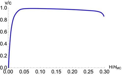
Figure 1: A plot of the $v(H)$ function constructed according to Eq. (13) at $p=10^{4}$, a part of the $v(H)$ curve $\left[(H/H_{MC})>0.2\right]$ requires further study since here the condition $\epsilon\ll 1$ is violated.

These equations determine the function $v(H)$ in the parametric form. The characteristic shape of this curve is given in Fig. 1. The maximum of this curve, which has the coordinates : $v_{m}=c(1-\sqrt{p})$, $H_{m}=H_{MC}p^{1/4}\left(1-\sqrt{p}\right)^{2}$, corresponds to $k_{m}=p^{1/2}(p\ll 1)$ and the point $H=0$, $v=0$ corresponds to $k_{m}=p^{1/6}(p\ll 1)$. The quantity $k_{m}/k_{0}\approx p^{1/4}$ characterizes the thickness ratio of the DB at $v=v_{m}$ and $v=0$. The function (13) coincides with Eq. (10) at $k_{0}<k<k_{m}$ or at $0<H<H_{m}$. The last inequality is the condition of applicability of Eqs. (8) and (10). The motion of the DB, in which $\bm{l}$ rotates in the $ac$ plane, is determined by more complicated equations than (6a) and (6b), but the function $v(H)$, which is determined by Eqs. (10), (13a), and (13b), remains valid in this case (if $d_{1}=-d_{3}$). In them it must be assumed that $\omega_{a}=\left(b_{1}-b_{3}\right)/M$.

IV

We give the numerical estimates. In YFeO₃ $A\approx 4\times 10^{-7}$ erg/cm, $H_{E}=6.4\times 10^{6}$ Oe, $H_{d}=10^{5}$ Oe, and $p\approx 10^{-4}$. The “scale” of the field H MC can be expressed in terms of the mobility $\mu$ when $H\rightarrow 0$: $\mu=\left(c/H_{MC}\right)p^{1/2}$. Hence, $H_{MC}=\left(c\sqrt{p}/\mu\right)$. According to Ref. [Uait, 1971], $\mu\simeq 5\times 10^{3}$ cm/sec$\cdot$Oe. Using these values, we obtain $c\approx 2\times 10^{6}$ cm/sec, $H_{MC}\approx 4\times 10^{4}$ Oe, $V_{m}=0.99$ s, and $H_{m}\approx 4\times 10^{3}$ Oe.

References

Note (1)For definiteness, we examine a crystal of rhombic
symmetry.
Walker and Dillon (1963)L. Walker and J. Dillon, Magnetism 3, 450
(1963).
Note (2)It has the same meaning as the well-known Walker’s
solution Walker and Dillon (1963) for ferromagnets, although its equations are more
complex.
Gyorgy and Hagedorn (1968)E. Gyorgy and F. Hagedorn, Journal of Applied Physics 39, 88 (1968).
Note (3)A similar dependence was obtained in Ref. [\rev@citealpnumgyorgy1968analysis], where the authors assumed that the
dynamics of the weak ferromagnetic moment are described by the same equations
as the dynamics of the ferromagnet and the magnetization remains constant
during the motion of the domain bounds.
Chetkin et al. (1977)M. Chetkin, A. Shalygin, and A. Kampa, Fizika Tverdogo
Tela 19, 3470 (1977).
Chetkin and de La Campa (1978)M. Chetkin and A. de La Campa, JETP Letters 27, 157
(1978).
Baryakhtar et al. (1978)V. Baryakhtar, B. Ivanov,
and A. Sukstanskii, Fizika Tverdogo
Tela 20, 2177 (1978).