Ab initio relaxation times and time-dependent Hamiltonians within the steepest-entropy-ascent quantum thermodynamic framework

Abstract

Quantum systems driven by time-dependent Hamiltonians are considered here within the framework of steepest-entropy-ascent quantum thermodynamics (SEAQT) and used to study the thermodynamic characteristics of such systems. In doing so, a generalization of the SEAQT framework valid for all such systems is provided, leading to the development of an ab initio physically relevant expression for the intra-relaxation time, an important element of this framework and one that had as of yet not been uniquely determined as an integral part of the theory. The resulting expression for the relaxation time is valid as well for time-independent Hamiltonians as a special case and makes the description provided by the SEAQT framework more robust at the fundamental level. In addition, the SEAQT framework is used to help resolve a fundamental issue of thermodynamics in the quantum domain, namely, that concerning the unique definition of process-dependent work and heat functions. The developments presented lead to the conclusion that this framework is not just an alternative approach to thermodynamics in the quantum domain but instead one that uniquely sheds new light on various fundamental but as of yet not completely resolved questions of thermodynamics.

I Introduction

The last three decades have seen experimental evidence (e.g., BRUN1 ; TURCH1 ; BOLL ; WALS ; CHUPP ; MAJU ; BENAT ; LISI ; KLAPD ; HOOP ; BATAL ) emerge at atomistic scales, which suggests the existence of irreversible changes even at these scales. Whether or not these changes are related to the measurement axiom of quantum mechanics (QM), the so-called “collapse of the wave function”, i.e., an abrupt collapse leading to irreversible change, or to something else entirely different is still a matter of debate. What is clear is that the collapse of the wave function postulate has drawn significant criticism EVER1 ; EVER2 ; MARG1 ; MARG2 ; PARK1 ; PARK2 ; GUERL ; GLEY ; SAYR and has led to an interpretation which replaces the abrupt collapse by a more gentle differentiable dynamical evolution. The result has been two theories, i.e., that of quantum open systems (QOS) KRAUS ; LIND ; GORI ; BREUER and that of typicality GEMM1 ; GOLD1 ; LUBK ; GOLD2 ; REIM ; POPE from which it is said that the Second Law of thermodynamics emerges. The former, which is a special case of the latter, relies on a partition between the primary system and the environment (e.g., the measuring device) and the total evolution in state is assumed to be unitary (i.e., linear) and generated by the Hamiltonian of the system-environment composite.

An alternative to an assumed collapse whether abrupt or more gradual is a possibly meaningful, nonlinear dynamics, which results when the postulates of QM are complemented by the Second Law, which, instead of emerging from QM, supplements it. In such an approach, the evolution of state can occur non-unitarily consistent with both the postulates of QM and thermodynamics. One such approach is that of intrinsic quantum thermodynamics (IQT) HATS1 ; HATS2 ; HATS3 ; HATS4 ; BERET1 ; SIMM ; BERET2 ; BERET3 ; BERET4 ; BERET5 and its mathematical framework steepest-entropy-ascent quantum thermodynamics (SEAQT) BERET6 ; BERET7 ; BERET8 ; BERET9 ; BERET10 ; LI1 ; LI2 ; LI3 ; CANO1 ; SMITH ; CANO2 ; LI4 ; LI5 ; BERET11 ; LI6 . It is this approach and the ones described above that are representative of the contrasting views of the origins of irreversible changes that form the basis of the field of quantum thermodynamics GEMM1 ; VINJ ; VONS1 , which has developed over the last four decades and has grown exponentially in the last decade and a half. In fact, the term quantum thermodynamics was first coined by Beretta et al. BERET1 ; SIMM ; BERET2 ; BERET3 ; BERET4 in the early 1980s with the publication of the dynamical aspects of IQT.

It is the mathematical framework of this latter theory, i.e., SEAQT, which is the basis of the developments presented here. Differing from other known approaches, the SEAQT framework results from a unified treatment of quantum mechanics and thermodynamics at a single level of description based on a generalized scheme of quantal dynamics in which the standard unitary dynamics governed by a given Hamiltonian is supplemented by a intra-dissipative (non-unitary) dynamics obtained from the requirement of maximum entropy production at every single instant of time. Remarkably enough, this enables the Second Law of thermodynamics to appear straightforwardly at a fundamental level of description (cf. for a contrasting view based on a quantum Maxwell demon, see LEB16 ; LES16 ; LLO97 ). As such, the SEAQT framework, which has been shown to encompass all of the well-known classical and quantum non-equilibrium frameworks BERET10 and is applicable even far from equilibrium, provides a conceptually consistent and mathematically and relatively compact framework for systematically analyzing non-equilibrium processes at any spatial and temporal scale. This first-principles, thermodynamic-ensemble-based approach has recently been extended via the concept of hypoequilibrium state and a corresponding set of intensive properties LI1 to provide the global features of the microscopic description as well as that of the nonequilibrium evolution of state of a system when combined with a set of nonequilibrium extensive properties. In contrast to the definitions of other nonequilibrium thermodynamic approaches, the SEAQT intensive property definitions are fundamental as opposed to phenomenological, are applicable to all nonequilibrium states, and enable the generalization of the equilibrium and near-equilibrium description (e.g., the Gibb’s relation, the Clausius inequality, the Onsager relations, and the quadratic dissipation potential) to the far-from-equilibrium realm. In addition, reduced computational burdens make the study of physically complex non-equilibrium phenomena at micro-scales possible where otherwise they may not be given the much heavier computational burdens associated with conventional approaches based purely on mechanics (i.e., quantum or classical) and/or stochastics (e.g., ensemble Monte Carlo). This framework can also facilitate the development of micro-scale analytical expressions, and its extension from the quantum to the classical regime is accomplished without resort to any extra (semi) classical approximations and manipulations, which are normally non-uniquely made. As a consequence, this approach provides a robust platform for exploring the thermodynamics of the quantal-classical transition regime and for affecting the scale-up of systems consisting of a few qubits to those of much greater extent, doing so with a single unified multi-scale thermodynamic picture of the kinematics and dynamics involved.

Both reactive and non-reactive quantum and classical systems have been investigated successfully using SEAQT LI1 ; LI2 ; LI3 ; CANO1 ; SMITH ; CANO2 ; LI4 ; LI5 ; BERET11 ; LI6 and some validations with experiment have been made CANO1 ; SMITH . It has furthermore been shown that not only does the equation of motion of SEAQT predict the unique thermodynamic path, which the system takes, BERET2 ; BERET3 but that the kinetics of this path (i.e., movement along it) and its dynamics (i.e., the time it takes for this movement) can be treated separately LI2 . Physically, this means that the system follows the same trajectory in state space regardless of the relaxation time $\tau$ chosen for the equation of motion. Whether a constant or a functional of the density operator $\hat{\rho}$ upon which the equation of motion is based, the dynamics of the process and, as a consequence a value for $\tau$, is determined via experiment CANO1 ; SMITH ; BERET11 or, for example, kinetic theory LI2 ; LI4 ; LI6 . What has been missing to date is $\tau$ as a functional of $\hat{\rho}$. Although Beretta BERET9 by analogy provides a lower limit for the relaxation time relative to the time-energy Heisenberg uncertainty principle, this limit does not in general, as has been shown in CANO1 ; SMITH ; CANO2 ; LI4 ; LI6 , provide a practical value for $\tau$. The purpose of the present paper is to provide such a functional and as a consequence a generalization of the SEAQT framework both for time-independent and time-dependent Hamiltonians. This development appears in Section IV. An added benefit of this development is that since the SEAQT framework inherently satisfies all the laws of mechanics and thermodynamics, generalized concepts for process-dependent heat and work transfers and process-independent internal energy changes in the quantum domain are provided. This appears in Section III and results in the First Law of thermodynamics and its resulting energy balance being uniquely well defined in the quantum domain, remarkably enough with the help of the Second Law, which the SEAQT framework embodies. We begin in Section II with an introduction to the SEAQT equation of motion and the limits placed on the relaxation times associated with the Hamiltonian and dissipation terms of this equation.

II Relaxation Time Limits and the SEAQT Equation of Motion

In the SEAQT framework for a single isolated system with a time-independent Hamiltonian, the time evolution of a density operator is given by BERET9

$$\frac{\partial\hat{\rho}}{\partial t}\,=\,\frac{i}{\hbar}\,[\hat{\rho},\hat{H}]+\hat{\mathbf{D}}_{1}(\hat{\rho},\hat{H},\{\hat{N}_{j}\})\,,$$ (1)

where $\hat{H}$ is the Hamiltonian, $\hat{\rho}$ the density or state operator, and $\hat{N}_{j}$ the $j$th particle number operator (or magnetic moment or other operator representing additional generators of the motion if any). The first term on the right-hand side governs the reversible dynamics conserving both the energy and entropy (the so-called von-Neumann term), while the second term describes the energy-conserving but internally entropy-generating and, thus, irreversible dynamics and is given by

$$\hat{\mathbf{D}}_{1}(\hat{\rho},\hat{H},\{\hat{N}_{j}\})\; =\;-\frac{1}{2\tau}\left[\sqrt{\hat{\rho}}\,\hat{D}+\hat{D}^{\dagger}\sqrt{\hat{\rho}}\right]$$ (1a)

$$\hat{D}\; =\;\left.\sqrt{\hat{\rho}}\,\hat{B}\,\ln(\hat{\rho})\right|_{\perp\,{\mathcal{L}}\{\sqrt{\hat{\rho}}\,\openone,\,\sqrt{\hat{\rho}}\,\hat{H},\,[\sqrt{\hat{\rho}}\,\hat{N}_{j}]\}}\,.$$ (1b)

In standard quantum mechanics, which neglects the entropy-generating term $\hat{\mathbf{D}}_{1}$, Eq. (1) obviously reduces to the well-known von-Neumann equation, giving rise to the unitary time evolution $\hat{\rho}(t)=\hat{U}\,\hat{\rho}(t_{0})\,\hat{U}^{\dagger}$ with $\hat{U}(t,t_{0})=e^{-i(t-t_{0})\hat{H}/\hbar}$. In (1a)-(1b) the intra-relaxation time $\tau=\tau(\hat{\rho})$ is a positive functional of $\hat{\rho}$, but has not uniquely been determined as of yet BERET9 . The idempotent operator $\hat{B}$ is introduced which assigns unity for each non-zero eigenvalue of $\hat{\rho}$, while zero for each vanishing eigenvalue of $\hat{\rho}$, thus, ensuring that the entropy operator $\hat{S}=-k_{\mbox{\tiny B}}\hat{B}\,\ln(\hat{\rho})$ is well-defined even when some eigenvalues of $\hat{\rho}$ vanish. By construction, the operator $\hat{D}$ is the component of $\hat{\mathbf{D}}_{1}$ perpendicular to the linear manifold ${\mathcal{L}}$ spanned by a set of operators $\{\sqrt{\hat{\rho}}\,\openone,\,\sqrt{\hat{\rho}}\,\hat{H},\,[\sqrt{\hat{\rho}}\,\hat{N}_{j}]\}$. The operator $\hat{\mathbf{D}}_{1}$ is then interpreted as driving the density operator $\hat{\rho}(t)$ at every instant of time in the direction of steepest entropy ascent ($ds/dt|_{\text{\tiny max}}>0$ with the entropy $s=-k_{\text{\tiny B}}\,\text{Tr}\{\hat{\rho}\,\ln\hat{\rho}\}$) relative to manifold specified by the time invariants $\{{\mathcal{U}}=\text{Tr}(\hat{\rho}\hat{H}),[{\mathcal{N}}_{j}=\text{Tr}(\hat{\rho}\hat{N}_{j})]\}$. Here ${\mathcal{U}}$ is the internal energy of the system and ${{\mathcal{N}}_{j}}$ the number of particles of the $j$th constituent.

Eq. (1) can be rewritten in the alternative form BERET9

$$\frac{\partial\hat{\rho}}{\partial t}=\sqrt{\hat{\rho}}\,\hat{E}(t)+\hat{E}^{\dagger}(t)\,\sqrt{\hat{\rho}}\,,$$ (2)

which will be used below. Here the decomposition $\hat{E}=\hat{E}_{H}+\hat{E}_{D}$ is composed of the von-Neumann part $\hat{E}_{H}=(i/\hbar)\sqrt{\hat{\rho}}\,\{\hat{H}+c(\hat{\rho})\openone\}$ corresponding to standard quantum mechanics with $c(\hat{\rho})\in{\mathbb{R}}$ being an arbitrary functional of $\hat{\rho}$ and the entropy-generating part $\hat{E}_{D}=-\hat{D}/(2\tau)$. As a consequence, the total dynamics given in (1) is non-unitary as long as the initial state $\hat{\rho}(t_{0})$ is in form of a mixed state. For any any pure state $\hat{\rho}(t_{0})=|\psi(t_{0})\rangle\langle\psi(t_{0})|$, the dynamics becomes unitary with $\hat{E}\to\hat{E}_{H}$. In this case, the operator $\hat{D}$ identically vanishes at every instant so that no entropy is generated during the time evolution. It is also straightforward to show that since $\sqrt{\hat{\rho}}$ is perpendicular to both components of $\hat{E}$,

$$0=\text{Tr}\left(\frac{\partial\hat{\rho}}{\partial t}\right)=\text{Tr}\left\{(\hat{E}+\hat{E}^{\dagger})\,\sqrt{\hat{\rho}}\right\}=2\,\left(\hat{E}|\sqrt{\hat{\rho}}\right)\,,$$ (3)

where the inner product $(\hat{F}|\hat{G})=\{\text{Tr}(\hat{F}^{\dagger}\hat{G}+\hat{G}^{\dagger}\hat{F})\}/2$ in symmetrized form is defined in the space $L({\mathcal{H}})$ of linear operators on the Hilbert space ${\mathcal{H}}$.

The operator $\hat{E}_{H}$ can directly be related to the time-energy uncertainty relation by first setting the real number $c(\hat{\rho})=-{\mathcal{U}}$ such that $\hbar^{2}(\hat{E}_{H}|\hat{E}_{H})=(\sqrt{\hat{\rho}}\,\Delta\hat{H}|\sqrt{\hat{\rho}}\,\Delta\hat{H})=\sigma^{2}_{\scriptscriptstyle H}$ with $\Delta\hat{H}=\hat{H}-{\mathcal{U}}\openone$ the deviation operator of $\hat{H}$ and $\sigma_{\scriptscriptstyle H}$ the standard deviation relative to $\hat{H}$ BERET9 . It then turns out that $\tau^{-2}_{\scriptscriptstyle H}:=4\,(\hat{E}_{H}|\hat{E}_{H})\geq\tau^{-2}_{\scriptscriptstyle A}$ with the help of the uncertainty relation $\sigma_{\scriptscriptstyle H}\,\tau_{\scriptscriptstyle A}\geq\hbar/2$ where the characteristic time $\tau_{\scriptscriptstyle A}$ for a given observable $\hat{A}$ (not explicitly time-dependent) may be interpreted as the amount of time it takes the expectation value of $\hat{A}$ to change by one standard deviation $\sigma_{\scriptscriptstyle A}=|d\langle\hat{A}\rangle/dt|\,\tau_{\scriptscriptstyle A}$ MES76 ; GRI05 . Accordingly, the time $\tau_{\scriptscriptstyle H}$, which results from the time-energy uncertainty relation with strict equality, is simply chosen above as the minimum value of the characteristic times, the $\tau_{\scriptscriptstyle A}$’s, for all possible observables, i.e., $\hat{A}$’s. Analogously, in BERET9 , it is assumed that the entropy-generating part $\hat{E}_{D}$ also satisfies the uncertainty relation, which renders the corresponding characteristic time $\tau_{\scriptscriptstyle D}=\tau\,(\hat{D}|\hat{D})^{-1/2}$ for which a value is found from the uncertainty equality BERET9 . This minimum value $(\tau_{\scriptscriptstyle D})_{\text{\tiny min}}$ provides the intra-relaxation time $\tau$ in question with its minimum value $\tau_{\text{\tiny min}}$.

However, this value $\tau_{\text{\tiny min}}$ has been shown to be significantly too small for generic experimental values of the relaxation time $\tau$, and so the substitution of $\tau_{\text{\tiny min}}$ into (1a) cannot be supported by the experimental data. Also theoretically, it has been verified that a minimum-uncertainty state must be a pure state STO72 ; BAL98 . In other words, the intra-relaxation time $\tau(\hat{\rho})$ for a mixed state $\hat{\rho}$ is required to be fundamentally greater than its minimum-uncertainty value. As a result, it is not physically consistent to impose the value $\tau_{\text{\tiny min}}$ upon the time evolution given in (2) for a generic mixed state. To address this, we introduce a different approach below for the determination of the intra-relaxation time, which is more physically relevant.

III Generalization of the SEAQT Equation of Motion for a Time-dependent Hamiltonian

Now to generalize Eq. (2) for the case of a time-dependent Hamiltonian $\hat{H}(t)$, the corresponding von-Neumann part $\hat{E}_{H}$ is first determined. From the von-Neumann equation valid also for this case, it easily follows that $\hat{E}_{H}=(i/\hbar)\sqrt{\hat{\rho}}\,\Delta\hat{H}(t)$, thus leading to

$$(\hat{E}_{H}|\sqrt{\hat{\rho}}\,\openone)=0\;\;;\;\;(\hat{E}_{H}|\sqrt{\hat{\rho}}\,\hat{H})=(\hat{E}_{H}|\sqrt{\hat{\rho}}\,\Delta\hat{H})=0\,.$$ (4)

Also note that $(\sqrt{\hat{\rho}}\,\openone|\sqrt{\hat{\rho}}\,\Delta\hat{H})=0$, i.e., these two operators are perpendicular to each other. It is also true that the energy-time uncertainty relation with the minimum-uncertainty equality holds true for this case (cf. KIM17 ). For purposes of comparison below, the unitary operator of time-evolution $\hat{U}(t)=\hat{T}e^{-i\int_{0}^{t}\hat{H}(t)/\hbar}$ of standard quantum mechanics obtained from the von-Neumann equation is briefly discussed. Here, the operator $\hat{T}$ denotes the time-ordering. In most of cases, it is a highly non-trivial exercise to derive a closed form expression for this operator. Nonetheless, it is instructive to transform this time-ordered form to an ordinary exponential form as in the case of a time-independent Hamiltonian. Thus, the exponential operator identity is applied such that LAM98

$$\hat{T}\,\exp\left\{\int_{0}^{t}d\tau\,\hat{\mathcal{B}}_{t}(\tau)\right\}\,=\,\exp\left\{\sum_{n=1}^{\infty}\hat{K}_{n}(t)\right\}\,,$$ (5)

where some of the lower-order terms are explicitly given by

$$\hat{K}_{1}(t)\,=\,\hat{C}_{1}(t)\;\;\; ;\;\;\;\hat{K}_{2}(t)\,=\,\frac{1}{2}\,\hat{C}_{2}(t)$$

$$\hat{K}_{3}(t)\,=\,\frac{1}{3}\,\hat{C}_{3}(t)+\frac{1}{12}\,\left[\hat{C}_{2}(t),\hat{C}_{1}(t)\right]\;\;\; ;\;\;\;\hat{K}_{4}(t)\,=\,\frac{1}{4}\,\hat{C}_{4}(t)+\frac{1}{12}\,\left[\hat{C}_{3}(t),\hat{C}_{1}(t)\right]\,.$$

Here the commutators are written as

$$\hat{C}_{n}(t)\,=\,\int_{0}^{t}d\tau_{1}\int_{0}^{\tau_{1}}d\tau_{2}\cdots\int_{0}^{\tau_{n-1}}d\tau_{n}\,\left[\hat{\mathcal{B}}_{t}(\tau_{1}),\left[\hat{\mathcal{B}}_{t}(\tau_{2}),\left[\cdots,\left[\hat{\mathcal{B}}_{t}(\tau_{n-1}),\hat{\mathcal{B}}_{t}(\tau_{n})\right]\cdots\right]\right]\right]\,,$$ (5b)

where $\hat{C}_{1}(t)=\int_{0}^{t}d\tau\,\hat{\mathcal{B}}_{t}(\tau)$ with $\hat{\mathcal{B}}_{t}(\tau)=-(i/\hbar)\hat{H}(\tau)$. In fact, the operators $\hat{K}_{n}(t)$ for all $n$ can be evaluated exactly. As an example of the time evolution in closed form, consider the two-level system given by $\hat{H}_{0}(t)=(\hbar\omega/2)\{\hat{\sigma}_{z}+a(t)\,\hat{\sigma}_{x}\}$ where the $\hat{\sigma}_{j}$’s denote Pauli matrices and a dimensionless quantity $a(t)\in{\mathbb{R}}$ is periodic in time $t$. The system’s time evolution is then explicitly given by $\hat{U}_{0}(t)=\hat{U}_{y}\,\utilde{\hat{U}}(t)\,\hat{U}_{y}^{\dagger}$ with $\hat{U}_{y}=e^{(i\pi/4)\,\hat{\sigma}_{y}}$ and the $(2\times 2)$ matrix $\utilde{\hat{U}}(t)$ by ARA84 ; HAE98 ; BAR00

$$\utilde{\hat{U}}(t)=\left(\begin{array}[]{ccc}R(t)\,\{1+i\,g_{0}\,S(t)\}&&-i\,\epsilon\,R(t)\,S(t)\\ -i\,\epsilon\,\bar{R}(t)\,\bar{S}(t)&&\bar{R}(t)\,\{1-i\,\bar{g}_{0}\,\bar{S}(t)\}\end{array}\right)\,,$$ (6)

where $\epsilon=\hbar\omega/2$, and $\bar{R}$, $\bar{S}$ and $\bar{g}_{0}$ denote the complex conjugates of $R$, $S$ and $g_{0}$, respectively. Here $R(t)=\exp[-i\int_{0}^{t}\,\{f(t^{\prime})+g(t^{\prime})\}\,dt^{\prime}]$, and $S(t)=\int_{0}^{t}\,\{R(t^{\prime})\}^{-2}\,dt^{\prime}$ where $f(t)=-(\hbar\omega/2)\,a(t)$ and $g(t)$, with $g_{0}=g(0)$, is a particular solution to the generalized Riccati equation $\partial_{t}\,g(t)-ig^{2}(t)-2if(t)\,g(t)+i\epsilon^{2}=0$ GRA07 .

Next, the corresponding entropy-generating part $\hat{E}_{D}$ of Eq. (2) is determined. To begin with, the energy balance of the First Law of thermodynamics is written as (see, e.g., ABE12 )

$$d{\mathcal{U}}=\sum_{n}{\mathcal{E}}_{n}\,dp_{n}+\sum_{n}p_{n}\,d{\mathcal{E}}_{n}\,,$$ (7)

where the ${\mathcal{E}}_{n}$’s are the eigenenergies and the $p_{n}$’s their respective probabilities. This balance provides a condition required for determining the direction of $\hat{E}_{D}$. The first term on the right is interpreted as the heat input $\delta Q_{\text{in}}$ from the environment and the second as the work $\delta W_{\text{in}}$ performed on the system (cf. see VIL08 ; VIL11 ; JAR08 for a discussion of the work for classical systems). Now, consider the case of a time-independent Hamiltonian. Accordingly, with no work input ($\delta W_{\text{in}}=0$), the balance reduces to $d{\mathcal{U}}=\delta Q_{\text{in}}$, and it is easily be shown with the help of (2) that

$$d{\mathcal{U}}/dt=\text{Tr}\{\hat{H}\,(d\hat{\rho}/dt)\}=2\left(\hat{E}\right.|\left.\sqrt{\hat{\rho}}\hat{H}\right)\,.$$ (8)

Therefore, for an isolated system with no heat exchange ($\delta Q_{\text{in}}=0$), $(\hat{E}|\sqrt{\hat{\rho}}\hat{H})=0$, which means that the two operators $\hat{E}$ and $\sqrt{\hat{\rho}}\hat{H}$ are perpendicular to each other. Subsequently, it is also straightforward to show that $(\hat{E}_{H}|\sqrt{\hat{\rho}}\hat{H})=0$ so that it follows that $(\hat{E}_{D}|\sqrt{\hat{\rho}}\hat{H})=0$ as well. Therefore, the invariance of ${\mathcal{U}}$ may simply be seen as resulting from the energy balance in a system with no heat nor work input. Likewise, for additional non-Hamiltonian invariants (if any),

$$d{\mathcal{N}}_{j}/dt=\text{Tr}\{\hat{N}_{j}\,(d\hat{\rho}/dt)\}=2\left(\hat{E}\right.|\left.\sqrt{\hat{\rho}}\hat{N}_{j}\right)\,,$$ (9)

and $d{\mathcal{N}}_{j}/dt$ also vanishes. With $(\hat{E}_{H}|\sqrt{\hat{\rho}}\hat{N}_{j})=0$, this results in $(\hat{E}_{D}|\sqrt{\hat{\rho}}\hat{N}_{j})=0$. Thus, it is seen that all invariants $\{{\mathcal{U}},[{\mathcal{N}}_{j}]\}$ uniquely determine the direction of $\hat{E}$.

Next, a similar scenario is developed for a system with no heat input but non-zero work input. For this case, the internal energy is no longer a time-invariant. In fact, it is assumed that there is no invariant available to the Hamiltonian system given by $\hat{H}(t)$. The quantity $\text{Tr}(\hat{H}d\hat{\rho})$, as given in (8), can then no longer be interpreted as $\delta Q_{\text{in}}$. To illustrate this, the aforementioned system $\hat{H}_{0}(t)$ is now considered. Its instantaneous eigenvalues and eigenvectors are explicitly given by

$${\mathcal{E}}_{1}(t)=(\hbar\omega/2)\sqrt{1+a^{2}(t)}\;\; \;\;|1(t)\rangle={\mathcal{N}}_{+}\left[a(t)|+\rangle+\{\sqrt{1+a^{2}(t)}-1\}|-\rangle\right]$$ ; (10a)

$${\mathcal{E}}_{2}(t)=-(\hbar\omega/2)\sqrt{1+a^{2}(t)}\;\; \;\;|2(t)\rangle={\mathcal{N}}_{-}\left[a(t)|+\rangle-\{\sqrt{1+a^{2}(t)}+1\}|-\rangle\right]\,.$$ ; (10b)

Here the (time-dependent) normalizing numbers are given by ${\mathcal{N}}_{\pm}=[2\,\{1+a^{2}(t)\mp\sqrt{1+a^{2}(t)}\}]^{-1/2}$ with the signs $+/-$ in accordance with their order on both sides. The internal energy is then shown to be ${\mathcal{U}}_{0}(t)=\text{Tr}(\hat{H}_{0}\hat{\rho})=\hbar\omega\,[\rho_{11}+a(t)\,\{\text{Re}(\rho_{12})\}-1/2]$ where the symbol $\rho_{jk}$ denotes the $(j,k)$-th component of a $(2\times 2)$-Hermitian matrix $\hat{\rho}$ and $\text{Re}(\rho_{12})$ is the real part of $\rho_{12}$. This easily yields $\text{Tr}(\hat{H}_{0}d\hat{\rho})=\hbar\omega\,[d\rho_{11}+a(t)\,d\{\text{Re}(\rho_{12})\}]$, while $\text{Tr}(\hat{\rho}\,d\hat{H}_{0})=\hbar\omega\{\text{Re}(\rho_{12})\}da$. In contrast, by expressing $\hat{\rho}$ within the instantaneous eigenbasis $\{|1(t)\rangle,|2(t)\rangle\}$ of $\hat{H}_{0}(t)$, its diagonal elements $p_{1}=1/2+[\rho_{11}+a\{\text{Re}(\rho_{12})\}-1/2]\,(1+a^{2})^{-1/2}$ and $p_{2}=1-p_{1}$ can straightforwardly be obtained. This gives

$$\delta Q_{\text{in}} = \sum_{n}{\mathcal{E}}_{n}\,dp_{n}\,=\,\hbar\omega\left[d\rho_{11}+d\{a\,\text{Re}(\rho_{12})\}-\frac{a\,\{\rho_{11}+a\,\text{Re}(\rho_{12})-1/2\}\,da}{1+a^{2}}\right]$$ (11a)

$$\delta W_{\text{in}} = \sum_{n}p_{n}\,d{\mathcal{E}}_{n}\,=\,\hbar\omega\left[\frac{a\,\{\rho_{11}+a\,\text{Re}(\rho_{12})-1/2\}\,da}{1+a^{2}}\right]\,.$$ (11b)

In this case, it is seen that $\delta Q_{\text{in}}\neq\text{Tr}(\hat{H}_{0}d\hat{\rho})$ and $\delta W_{\text{in}}\neq\text{Tr}(\hat{\rho}\,d\hat{H}_{0})$. Thus, the association of $\delta Q_{\text{in}}$ with $\text{Tr}(\hat{H}_{0}d\hat{\rho})$ and $\delta W_{\text{in}}$ with $\text{Tr}(\hat{\rho}\,d\hat{H}_{0})$ as is routinely done in the literature (cf. VONS1 ; GEMM1 ) is not warranted for the case of a time-dependent Hamiltonian.

IV Formal Development of the Relaxation Time Functional

The previous generalization is now discuss more systematically. To do so, consider

$$\delta\lambda(t):=\text{Tr}\{\hat{H}(t)\,d\hat{\rho}\}=\sum_{n}{\mathcal{E}}_{n}\,\langle n|(d\hat{\rho})|n\rangle\,,$$ (12)

expressed in terms of the instantaneous eigenvectors $\{|n\rangle\}$ of $\hat{H}(t)$. From the identity that $\langle n|(d\hat{\rho})|n\rangle=d(\langle n|\hat{\rho}|n\rangle)-(d\langle n|)\hat{\rho}|n\rangle-\langle n|\hat{\rho}(d|n\rangle)$ with $d(\langle n|\hat{\rho}|n\rangle)=dp_{n}$, it is easily seen that $\delta\lambda\neq\delta Q_{\text{in}}=\sum_{n}{\mathcal{E}}_{n}dp_{n}$ for $\hat{H}(t)$ whereas $\delta\lambda=\delta Q_{\text{in}}$ for its time-independent counterpart. Thus, for the case of $\delta Q_{\text{in}}=0$ and a time-dependent Hamiltonian, $\delta\lambda\neq 0$ always. Based on Eq. (8), this leads to the conclusion that $\hat{E}$ is not perpendicular to $\sqrt{\hat{\rho}}\,\hat{H}(t)$, which means that the procedure following Eq. (8) above for determining the direction of $\hat{E}$ cannot be employed. However, as seen from (4), the von-Neumann part $\hat{E}_{H}$ remains perpendicular to $\sqrt{\hat{\rho}}\,\hat{H}(t)$; and as a consequence, without the intra-entropy-generation provided by the SEAQT framework (i.e., with $\hat{E}\to\hat{E}_{H}$), one must conclude that $\text{Tr}\{\hat{H}(t)\,(d\hat{\rho}/dt)\}=2\,(\hat{E}_{H}|\sqrt{\hat{\rho}}\,\hat{H})=0$ [cf. (12)], which necessarily contradicts $\delta\lambda\neq 0$ or $\delta Q_{\text{in}}=0$. This is a fundamental conceptual problem within the thermodynamics embedded in the scheme of standard quantum mechanics. Furthermore, the entropy-generating part $\hat{E}_{D}$ cannot be perpendicular to $\sqrt{\hat{\rho}}\,\hat{H}(t)$ for the case of a time-dependent Hamiltonian or else $\delta\lambda=0$, resulting in $\delta Q_{\text{in}}\neq 0$ which again is a contradiction.

To resolve this conceptual inconsistency and as a result develop a consistent thermodynamics of the quantum domain, the intra-entropy-generation available in SEAQT is used to uniquely determine the direction of $\hat{E}_{D}$ and as a consequence that of $\hat{E}$. To that end, it is again assumed that $\delta Q_{\text{in}}=0$, i.e.,

$$\sum_{n}\left(\frac{d}{dt}\langle n|\hat{\rho}|n\rangle\right)\,{\mathcal{E}}_{n}\stackrel{{\scriptstyle!}}{{=}}0\,,$$ (13)

so that from the energy balance, $d{\mathcal{U}}=\delta W_{\text{in}}$. Eq. (13) is subsequently rewritten as

$$\sum_{n}\left\langle n|(d\hat{\rho}/dt)|n\right\rangle\,{\mathcal{E}}_{n}=-2\sum_{n}\text{Re}\left\{\langle n|\hat{\rho}\,(d/dt)|n\rangle\right\}\,{\mathcal{E}}_{n}\,.$$ (13a)

The left-hand side is nothing else than $\text{Tr}\{\hat{H}(t)\,(d\hat{\rho}/dt)\}=2\,(\hat{E}|\sqrt{\hat{\rho}}\,\hat{H})$ as discussed above. With the help of $(\hat{E}_{H}|\sqrt{\hat{\rho}}\,\hat{H})=0$, Eq. (13a) reduces to

$$(\hat{E}_{D}|\sqrt{\hat{\rho}}\,\hat{H})=-\text{Re}\sum_{n}{\langle n|\hat{\rho}\,(d/dt)|n\rangle}\,{{\mathcal{E}}_{n}}\,,$$ (13b)

where the right-hand side is non-vanishing in contrast to its counterpart for the time-independent Hamiltonian, which vanishes. Substituting the identity of completeness $\sum_{m}|m\rangle\langle m|=\openone$ into the right-hand side of (13b), recognizing that $\langle n|\partial_{t}|n\rangle$ is purely imaginary as a result of $\langle n|\partial_{t}|n\rangle+\langle\partial_{t}n|n\rangle=0$, and then applying the relation of instantaneous eigenstates given by GON13

$$\langle m|\partial_{t}|n\rangle=\langle m|\{\partial_{t}\hat{H}(t)\}|n\rangle/({\mathcal{E}}_{n}-{\mathcal{E}}_{m})$$ (14)

which is valid for $m\neq n$, one finally obtains the exact expression

$$(\hat{E}_{D}|\sqrt{\hat{\rho}}\,\hat{H})\;=\;-\text{Re}\sum_{n}\sum_{m\,(\neq n)}\rho_{nm}\,\langle m|\{\partial_{t}\hat{H}(t)\}|n\rangle/(1-{\mathcal{E}}_{m}/{\mathcal{E}}_{n})\,.$$ (13c)

For simplicity, it is assumed here that the system is non-degenerate (${\mathcal{E}}_{n}\neq{\mathcal{E}}_{m}$ if $n\neq m$). Eq. (13c) can then be rewritten in terms of the commutator $[\;,\;]_{-}$ as

$$(\hat{E}_{D}|\sqrt{\hat{\rho}}\,\hat{H})\;=\;\sum_{n}\sum_{m\,(\neq n)}\frac{\rho_{nm}}{2\,({\mathcal{E}}_{n}-{\mathcal{E}}_{m})}\;\langle m|\left[\hat{H},\{\partial_{t}\hat{H}(t)\}\right]_{-}|n\rangle\,.$$ (13d)

It should be noted that Eq. (13d) can straightforwardly be generalized to a system with a continuous energy spectrum ILK17 . Furthermore, the validity of (13d) can easily be verified from the previous example for $\hat{H}_{0}(t)$ in such a way that the left-hand side of (13d) is explicitly given by

$$(\hat{E}_{D}|\sqrt{\hat{\rho}}\,\hat{H})=\frac{1}{2}\sum_{n}\langle n|(d\hat{\rho}/dt)|n\rangle\;{\mathcal{E}}_{n}=\frac{\hbar\omega}{2}\,\{\partial_{t}\,\rho_{11}+a(t)\,\text{Re}(\partial_{t}\,\rho_{12})\}\,$$ (15a)

and the right-hand side becomes

$$\frac{1/2}{{\mathcal{E}}_{1}-{\mathcal{E}}_{2}}\,\left\{\rho_{12}\,\langle 2|\left[\hat{H},\{\partial_{t}\hat{H}(t)\}\right]_{-}|1\rangle-\rho_{21}\,\langle 1|\left[\hat{H},\{\partial_{t}\hat{H}(t)\}\right]_{-}|2\rangle\right\}$$ (15b)

which can immediately be reduced to $\hbar\omega\dot{a}\,\{4\,(1+a^{2})\}^{-1}\,\{2a\,\rho_{11}-a+2a^{2}\,\text{Re}(\rho_{12})\}$ where $\rho_{12}=\langle 1|\hat{\rho}|2\rangle$ with $|1\rangle$ and $|2\rangle$ explicitly given by (10a)-(10b). The equality of this last expression with the right-hand-side of Eq. (15a) confirms that $\delta Q_{\text{in}}=0$ in (11a), which is consistent with the assumption of no heat transfer for this system.

For purposes of the development below, Eq. (13c) is now rewritten by first noting that Eq. (3) is also valid for a generic time-dependent Hamiltonian. With the help of (4), this immediately yields that $(\hat{E}_{D}|\sqrt{\hat{\rho}})=0$. Therefore, a real functional $c(\hat{\rho})$ can be introduced such that $(\hat{E}_{D}|\sqrt{\hat{\rho}}\,\hat{H})=(\hat{E}_{D}|\sqrt{\hat{\rho}}\,\{\hat{H}+c(\hat{\rho})\,\openone\})$. Consistent with the case for a time-independent Hamiltonian, the real functional $c(\hat{\rho})$ is set equal to $-{\mathcal{U}}(t)$. Two normalized operators are introduced next such that $\hat{z}:=\hat{E}_{D}/\{(\hat{E}_{D}|\hat{E}_{D})\}^{1/2}$ with $(\hat{z}|\hat{z})=1$ and $\hat{h}:=\sqrt{\hat{\rho}}\,(\Delta\hat{H})/\sigma_{\scriptscriptstyle H}$ with $(\hat{h}|\hat{h})=1$ where the standard deviation $\sigma_{\scriptscriptstyle H}(t)=\{(\sqrt{\hat{\rho}}\,\Delta\hat{H}|\sqrt{\hat{\rho}}\,\Delta\hat{H})\}^{1/2}$ as in the time-independent Hamiltonian case. Then, $(\hat{E}_{D}|\sqrt{\hat{\rho}}\,\Delta\hat{H})=\{(\hat{E}_{D}|\hat{E}_{D})\}^{1/2}\,\sigma_{\scriptscriptstyle H}\,\cos(\theta_{zh})$ where $\cos\theta_{zh}=(\hat{z}|\hat{h})$. This enables Eq. (13c) to be transformed into

$$\cos\theta_{zh}=\frac{\Lambda(t)}{\{(\hat{E}_{D}|\hat{E}_{D})\}^{1/2}\,\sigma_{\scriptscriptstyle H}}\,,$$ (16)

where $\Lambda(t)=\text{Re}\sum_{n}\sum_{m\,(\neq n)}\rho_{nm}\,\langle m|\{\partial_{t}\,\hat{H}(t)\}|n\rangle\,({\mathcal{E}}_{m}/{\mathcal{E}}_{n}-1)^{-1}$. This last equation can be used to determine the direction of $\hat{E}_{D}$ as long as the magnitude $\{(\hat{E}_{D}|\hat{E}_{D})\}^{1/2}$ is known. In fact, it is seen from this generalization to the case of a time-dependent Hamiltonian that the time-independent Hamiltonian case exactly corresponds as required to the special case of $\theta_{zh}=\pi/2$. Note also that for the system $\hat{H}_{0}(t)$ given in (10a)-(10b), Eq. (3) holds true, and $(\sqrt{\hat{\rho}}\,\hat{H}_{0}|\sqrt{\hat{\rho}}\,\hat{H}_{0})=\text{Tr}[\hat{\rho}(t)\,\{\hat{H}_{0}(t)\}^{2}]=\{{\mathcal{E}}_{1}(t)\}^{2}$ explicitly so that the variance is given by

$$\{\sigma_{\scriptscriptstyle H}(t)\}^{2}=(\hbar\omega/2)^{2}\,\left[\{a(t)\}^{2}-4\,\{\upsilon_{0}(t)\}^{2}+4\,\upsilon_{0}(t)\right]\,,$$ (17)

where the dimensionless quantity $\upsilon_{0}(t)=\rho_{11}(t)+a(t)\,\text{Re}\{\rho_{12}(t)\}=1/2+{\mathcal{U}}_{0}(t)/\hbar\omega$.

Now, before exploring an explicit evaluation for $(\hat{E}_{D}|\hat{E}_{D})$, the quantity $(\hat{D}|\hat{D})=4\,\tau^{2}\,(\hat{E}_{D}|\hat{E}_{D})$, which is more straightforward to evaluate, is first considered. Then with the help of (1b),

$$\hat{D} = \left.\sqrt{\hat{\rho}}\,\hat{B}\,\ln(\hat{\rho})\right|_{\perp\,{\mathcal{L}}\{\sqrt{\hat{\rho}}\,\openone,\,\sqrt{\hat{\rho}}\,\hat{\Upsilon}\}}$$ (18)

$$= \sqrt{\hat{\rho}}\,\hat{B}\,\ln(\hat{\rho})-\left\{(\sqrt{\hat{\rho}}\,\hat{B}\,\ln\hat{\rho}|\sqrt{\hat{\rho}})\,\sqrt{\hat{\rho}}\,\openone\,+\,(\sqrt{\hat{\rho}}\,\hat{B}\,\ln{\hat{\rho}}|\sqrt{\hat{\rho}}\,\Delta\hat{\utilde{\Upsilon}})\,\sqrt{\hat{\rho}}\,\Delta\hat{\utilde{\Upsilon}}\right\}\,,$$

where the operator $\sqrt{\hat{\rho}}\,\hat{\Upsilon}(t)$ is described in what follows. Thus, using $\Delta\hat{\utilde{\Upsilon}}(t)=\hat{\Upsilon}(t)-(\sqrt{\hat{\rho}}\,\hat{\Upsilon}|\sqrt{\hat{\rho}})\,\openone$ with $(\sqrt{\hat{\rho}}\,\Delta\hat{\utilde{\Upsilon}}|\sqrt{\hat{\rho}}\,\Delta\hat{\utilde{\Upsilon}})=1$ guarantees that the two operators $\sqrt{\hat{\rho}}\,\openone$ and $\sqrt{\hat{\rho}}\,\Delta\hat{\utilde{\Upsilon}}(t)$ are orthonormal to each other so that $(\sqrt{\hat{\rho}}\,\Delta\hat{\utilde{\Upsilon}}|\sqrt{\hat{\rho}}\,\openone)=0$ at every instant of time. To visualize the behavior of $\sqrt{\hat{\rho}}\,\hat{\Upsilon}(t)$, a three-dimensional space of linear operators spanned by the orthonormal basis $\{\hat{x}\to\sqrt{\hat{\rho}}\,\openone;\,\hat{y}\to\sqrt{\hat{\rho}}\,\Delta\hat{\utilde{\Upsilon}};\,\hat{z}\to\utilde{\hat{E}}_{D}\}$ with $\utilde{\hat{E}}_{D}=\hat{E}_{D}/\{({\hat{E}}_{D}|{\hat{E}_{D}})\}^{1/2}=-\hat{D}/\{(\hat{D}|\hat{D})\}^{1/2}$ is introduced as illustrated in Fig. 1. This means that the operator $\sqrt{\hat{\rho}}\,\Delta\hat{\utilde{\Upsilon}}(t)$ is chosen so that $(\sqrt{\hat{\rho}}\,\Delta\hat{\utilde{\Upsilon}}|\utilde{\hat{E}}_{D})=0$. This three-dimensional space enables a linear operator to be specified by its components $(x,y,z)$. For example, for $\sqrt{\hat{\rho}}\,\hat{B}\,\ln\hat{\rho}$ given in (18), $x=(\sqrt{\hat{\rho}}\,\hat{B}\,\ln\hat{\rho}|\hat{x})<0$, $y=(\sqrt{\hat{\rho}}\,\hat{B}\,\ln\hat{\rho}|\hat{y})$, and $z=(\sqrt{\hat{\rho}}\,\hat{B}\,\ln\hat{\rho}|\hat{z})<0$. The decomposition $\sqrt{\hat{\rho}}\,\Delta\hat{H}(t)=(\sqrt{\hat{\rho}}\,\Delta\hat{H}|\hat{y})\,\hat{y}+(\sqrt{\hat{\rho}}\,\Delta\hat{H}|\hat{z})\,\hat{z}$ then follows where $\sqrt{\hat{\rho}}\,\Delta\hat{H}(t)/\sigma_{\scriptscriptstyle H}$ is represented by $\hat{h}$ in Fig. 1 and $(\sqrt{\hat{\rho}}\,\Delta\hat{H}|\hat{z})=\sigma_{\scriptscriptstyle H}\,\cos\theta$ and $(\sqrt{\hat{\rho}}\,\Delta\hat{H}|\hat{y})=\pm\sigma_{\scriptscriptstyle H}\,\sin\theta$. Therefore, the angle $\theta_{zh}(t)$ given in (16) is geometrically seen as the polar angle $\theta(t)$ of this operator space. Furthermore, using the decomposition for $\sqrt{\hat{\rho}}\,\Delta\hat{H}(t)$ given above and the assignments for $(\hat{h},\hat{y},\hat{z})$ depicted above and in Fig. 1,

$$\hat{y}=\{\hat{h}-(\cos\theta)\,\hat{z}\}/(\pm\sin\theta),$$ (19)

which can be interpreted as the projection of $\sqrt{\hat{\rho}}\,\hat{\Upsilon}(t)$ onto the $y$-axis. As a consequence, $\hat{D}\propto-\hat{z}$, which accordingly is perpendicular to the $(xy)$-plane of this operator space as required.

The magnitude of $\hat{D}$, which is now explicitly evaluated, easily with the help of (18) reduces to

$$\{(\hat{D}|\hat{D})\}^{1/2}=\{(\sigma_{\scriptscriptstyle\ln\rho})^{2}-(\sqrt{\hat{\rho}}\,[\hat{B}\,\ln\hat{\rho}-\eta\,\openone]|\hat{y})\}^{1/2}\,,$$ (20)

where $\eta=(\sqrt{\hat{\rho}}\,\hat{B}\,\ln\hat{\rho}|\sqrt{\hat{\rho}})=-s/k_{\text{\tiny B}}$, $s=-k_{\text{\tiny B}}\,\text{Tr}(\hat{\rho}\,\ln\hat{\rho})$, and the variance $(\sigma_{\scriptscriptstyle\ln\rho})^{2}=\text{Tr}\{\hat{\rho}\,(\ln\hat{\rho})^{2}\}-\eta^{2}$ with $\sigma_{\scriptscriptstyle\ln\rho}=\sigma_{\scriptscriptstyle s}/k_{\text{\tiny B}}$. Eq. (19) is next substituted into (20) and the relations $\cos\theta=-(\hat{D}|\hat{h})/\{(\hat{D}|\hat{D})\}^{1/2}$ and $(\hat{D}|\hat{D})=(\sqrt{\hat{\rho}}\,\{\hat{B}\,\ln\hat{\rho}-\eta\,\openone\}|\hat{D})$ applied. After some algebraic manipulations, the following quadratic equation in compact form is found: $\chi^{2}+2\alpha\,(\cos\theta)\,\chi-\{(\sin\theta)\,\sigma_{\scriptscriptstyle\ln\rho}\}^{2}+\alpha^{2}=0$ where $\chi=(\hat{D}|\hat{D})^{1/2}$ and $\alpha(\theta)=(\sqrt{\hat{\rho}}\,\{\hat{B}\,\ln\hat{\rho}-\eta\,\openone\}|\hat{h})$ with $(\sigma_{\scriptscriptstyle\ln\rho})^{2}\geq\alpha^{2}$. This easily yields that

$$\chi_{\pm}(\theta)\,=\,-\alpha\,(\cos\theta)\pm(\sin\theta)\,\{(\sigma_{\scriptscriptstyle\ln\rho})^{2}-\alpha^{2}\}^{1/2}\,,$$ (21)

where the signs $+/-$ are in accordance with their order on both sides and $\chi_{+}\geq\chi_{-}$. Substituting the two roots $\chi_{\pm}$ into (20), it is concluded that $\chi_{+}>0$ is the only allowed solution consistent with the requirement that $\{(\sin\theta)\,\sigma_{\scriptscriptstyle\ln\rho}\}^{2}>\{\alpha(\theta)\}^{2}$. For the case of $\theta=\pi/2$ at a given instant of time, $\chi_{+}(\pi/2)=[(\sigma_{\scriptscriptstyle\ln\rho})^{2}-\{\alpha(\pi/2)\}^{2}]^{1/2}$, which corresponds to the case of the time-independent Hamiltonian. In contrast, if $\theta=0$ or $\pi$ at a given instant of time, then $\alpha=0$ and $\chi_{+}=0$, which corresponds to the case of no entropy-generation.

The inner product $(\hat{E}_{D}|\hat{E}_{D})$ is now determined by first considering the inequality given by $\{(\hat{E}_{D}|\hat{E}_{D})\}^{1/2}\geq(\hat{E}_{D}|\hat{h})=(\cos\theta_{zh})\,\{(\hat{E}_{D}|\hat{E}_{D})\}^{1/2}$. Recall that Eqs. (13a)-(13d) have been obtained directly from Eq. (13), which is physically relevant since it is required by thermodynamics and by the actual dynamics of the density operator $\hat{\rho}$ of (2). In fact, they are the only available expressions, which implicitly contain information on the magnitude of the dynamics of the operator $\hat{E}_{D}$. Motivated by this fact, an approach can now be proposed to determine $(\hat{E}_{D}|\hat{E}_{D})$ in such a way that without changing the Hamiltonian $\hat{H}(t)$ and the internal energy ${\mathcal{U}}(t)$ at time $t$, $|(\hat{E}_{D}|\hat{h})|$ is maximized by replacing $\hat{\rho}(t)$ with all possible density matrices ($\hat{\varrho}$’s) that have the same entropy $s(t)=-k_{\text{\tiny B}}\,\text{Tr}\{\hat{\rho}(t)\,\ln\hat{\rho}(t)\}$ (or with the purity $\mu(t)=\text{Tr}\{\hat{\rho}^{2}(t)\}$ in a weaker form). The maximum value $(\hat{E}_{D}|\hat{h})_{\mbox{\tiny max}}$ at time $t$ is then identified as $\{(\hat{E}_{D}|\hat{E}_{D})\}^{1/2}$, which is subsequently substituted into (16) to determine the angle $\theta_{zh}(t)$. Here it is stressed that, when the angle $\tilde{\theta}_{zh}=0$ in this identification, it does not represent the actual angle $\theta_{zh}=0$ between $\hat{E}_{D}$ and $\hat{h}$ which simply corresponds to the case when $\hat{E}_{D}=0$ (i.e., $\chi_{+}=0$) as discussed in the previous paragraph.

The intra-relaxation time $\tau=\{(\hat{D}|\hat{D})\}^{1/2}/[2\,\{(\hat{E}_{D}|\hat{E}_{D})\}^{1/2}]$ determined by this approach is more physically relevant than its minimum-uncertainty counterpart since the former reflects the actual dynamics of the density operator $\hat{\rho}(t)$ in terms of $\mu(t)$, especially for a mixed state $\hat{\rho}(t)$ with $\mu(t)<1$. The detailed development for $\tau$ is given below. Therefore, this value of the relaxation time is necessarily greater than the minimum-uncertainty value corresponding to a pure state only (more precisely, to the (instantaneous) ground state of the system considered). The latter time is completely irrelevant to the actual dynamics. As a consequence, it is argued here that the maximizing process proposed above for determining the magnitude and direction of $\hat{E}_{D}$ (and, thus, the magnitude of $\tau$) must be regarded as an important addition to the SEAQT framework, one not considered thus far even for the case of a time-independent Hamiltonian.

The inner product $(\hat{E}_{D}|\hat{E}_{D})$ is now determined for the example $\hat{H}_{0}(t)$ previously used. With the help of (15a) and (17), it is straightforward to obtain

$$(\hat{E}_{D}|\hat{h})=\frac{\partial_{t}\,\upsilon_{0}(t)-\{\text{Re}(\rho_{12})\}\,\partial_{t}\,a(t)}{[\{a(t)\}^{2}-4\,\{\upsilon_{0}(t)\}^{2}+4\,\upsilon_{0}(t)]^{1/2}}\,.$$ (22)

For a fixed purity $\mu_{0}(t)=(\rho_{11})^{2}+(\rho_{22})^{2}+2\,|\rho_{12}|^{2}$ at time $t$, the right-hand side of (22) is maximized by finding an optimal value of $\text{Re}(\varrho_{12})$ to replace $\text{Re}\{\rho_{12}(t)\}$. To do so, the maximum value $\{\text{Re}(\rho_{12})\}^{2}_{\mbox{\tiny max}}$, which minimizes $(\rho_{11})^{2}+(\rho_{22})^{2}$ in the purity measure, is found, resulting in $\rho_{11}=\rho_{22}=1/2$. It then follows that $\{\text{Re}(\rho_{12})\}^{2}_{\mbox{\tiny max}}=[2\,\mu_{0}(t)-1-4\,\{\text{Im}(\rho_{12})\}^{2}]/4$. The maximum of this maximum, $\{\text{Re}(\rho_{12})\}^{2}_{\mbox{\tiny max,max}}$, occurs with $\text{Im}(\rho_{12})=0$. $\{\text{Re}(\varrho_{12})\}^{2}=\{\text{Re}(\rho_{12})\}^{2}_{\mbox{\tiny max,max}}$ is then substituted for $\text{Re}(\rho_{12})$ in (22) and the inequality $r_{1}+r_{2}\leq|r_{1}|+|r_{2}|$ used for two real numbers $r_{1}$ and $r_{2}$ to arrive at

$$(\hat{E}_{D}|\hat{E}_{D})^{1/2}=\frac{|\partial_{t}\,\upsilon_{0}(t)|+|\{\text{Re}(\varrho_{12})\}\,\partial_{t}\,a(t)|}{[\{a(t)\}^{2}-4\,\{\upsilon_{0}(t)\}^{2}+4\,\upsilon_{0}(t)]^{1/2}}$$ (23)

where the two constraints on $\upsilon_{0}$, i.e., ${\mathcal{U}}_{0}$ with $a(t)$, and $\mu_{0}$ hold. By substituting (23) into (16), the direction of $\hat{E}_{D}$ denoted by $(\theta_{zh})_{0}$ can be determined.

Based on the above analysis, the internal-relaxation time can be uniquely determined. Using (16) in (21) results in

$$\tau(\hat{\rho})=\frac{\chi_{+}}{2\,\{(\hat{E}_{D}|\hat{E}_{D})\}^{1/2}}=\frac{-\alpha\,\Lambda+(\chi_{+,0})\,\{(\hat{E}_{D}|\hat{E}_{D})\,\sigma_{\scriptscriptstyle H}^{2}-\Lambda^{2}\}^{1/2}}{2\,\sigma_{\scriptscriptstyle H}\,(\hat{E}_{D}|\hat{E}_{D})}\,,$$ (24)

where $\chi_{+,0}(\theta_{zh})=[(\sigma_{\scriptscriptstyle\ln\rho})^{2}-\{\alpha(\theta_{zh})\}^{2}]^{1/2}$ and $(\hat{E}_{D}|\hat{E}_{D})$ is found from the maximization process described above. Therefore, all quantities on the right-hand side of (21) can be evaluated. Obviously, Eq. (24) is also valid for the special case of a time-independent Hamiltonian for which $\theta_{zh}=\pi/2$ and $\Lambda=0$, leading to $\tau\to\{\chi_{+}(\pi/2)\}\,[2\,\{(\hat{E}_{D}|\hat{E}_{D})\}^{1/2}]^{-1}$, which is clearly different from its minimum-uncertainty counterpart $\hbar\,(2\,\sigma_{\scriptscriptstyle H})^{-1}$. As seen in (24) [cf. $\Lambda(t)$], the off-diagonal terms of the density matrix play a critical role in determining $\tau(\hat{\rho})$. In contrast, the minimum-uncertainty value results from the ground (minimum-energy) pure state for which the off-diagonal terms are identically zero. For the more general case of $\theta_{zh}\neq\pi/2$ and $\Lambda\neq 0$ (i.e., for the case of the time-dependent Hamiltonian) and with the help of (16), the expression for $\tau$ can be rewritten as

$$\tau(\hat{\rho})=-(\hat{D}|\sqrt{\hat{\rho}}\,\Delta\hat{H})\,\{2\,\Lambda(t)\}^{-1}\,,$$ (25)

where $(\hat{D}|\sqrt{\hat{\rho}}\,\Delta\hat{H})=-\{(\hat{D}|\hat{D})\}^{1/2}\,\sigma_{\scriptscriptstyle H}\,(\cos\theta_{zh})$.

V Conclusions

The preceding development, which is based on a formal consideration of time-dependent Hamiltonians ($\hat{H}(t)$’s), is a generalization of the SEAQT framework that results in ab initio expressions for the intra-relaxation time. The latter is an important element of this framework, one which had not previously been uniquely determined as an integral part of the theory. The approach proposed here to determine $\tau{(\hat{\rho})}$ is a physically relevant one based on an additional maximization process, i.e. one that supplements the steepest-entropy-ascent maximization, which forms the basis of the SEAQT framework. The expressions developed are valid for both time-dependent and time-independent Hamiltonians and transform the description provided by this framework into an even more robust one at the fundamental level.

The other significant development provided here is that of critically contributing to a resolution of a fundamental issue of thermodynamics in the quantum domain concerning the unique definition of process-dependent work and heat functions. This is done with the aid of the SEAQT framework and the energy balance resulting from the first law of thermodynamics. As is well-known, this conceptual problem has been an open question within the thermodynamics embedded in the standard quantum mechanics approach when both work, as given by an explicitly time-dependent Hamiltonian, and heat are simultaneously considered. It is this latter development, which will be a particular focus of a future paper. An additional focus will be the numerical application of our framework to a number of driven quantum systems such as the two-level system with $\hat{H}_{0}(t)$ introduced in Section III and a linear oscillator with a time-dependent frequency. These applications will take advantage of the fact that the numerical implementation of the SEAQT framework has thus far been very robust for the case of time-independent Hamiltonians.

Finally, a consequence of the developments given here is that SEAQT is not just an alternative approach to thermodynamics in the quantum domain but in fact sheds new light on the various fundamental but not completely resolved questions of thermodynamics. It is also expected that these new developments will contribute to providing foundational guidance for driven thermodynamic machines operating in the quantum/nano domain.

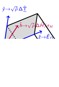
Figure 1:

Fig. 1: (Color online) The three-dimensional space of linear operators whose basis consists of the three orthonormal operators $\{\hat{x}=\sqrt{\hat{\rho}}\,\openone;\,\hat{y}=\sqrt{\hat{\rho}}\,\Delta\hat{\utilde{\Upsilon}};\,\hat{z}=\utilde{\hat{E}}_{D}\}$ [cf. after Eq. (18)]. Here the normalized operator $\hat{h}=(\sin\theta)\,\hat{y}+(\cos\theta)\,\hat{z}=\sqrt{\hat{\rho}}\,\Delta\hat{H}(t)/\sigma_{\scriptscriptstyle H}$ lying on the $(yz)$-plane, expressed in terms of the polar angle $\theta$ of the spherical coordinate system $(r,\theta,\varphi)$, where $0\leq\theta\leq\pi$, and $\sin\theta=(\hat{h}|\hat{y})$ and $\cos\theta=(\hat{h}|\hat{z})$.

References

- (1) M. Brune, E. Hagley, J. Dreyer, X. Maitre, A. Maali, Ch. Wunderlich, J. M. Raimond, and S. Haroche, Observing the progressive decoherence of the “meter” in a quantum measurement, Phys. Rev. Lett. 77, 4887 (1996).
- (2) Q. A. Turchette, C. J. Myatt, B. E. King, C. A. Sackett, D. Kielpinski, W. M. Itano, Ch. Monroe, and D. J. Wineland, Decoherence and decay of motional quantum states of a trapped atom coupled to engineered reservoirs, Phys. Rev. A 62, 053807 (2000).
- (3) J. J. Bollinger, D. J. Heinzen, W. M. Itano, S. L. Gilbert, and D. J. Wineland, Test of the linearity of quantum mechanics by rf spectroscopy of the 9Be+ ground state, Phys. Rev. Lett. 63, 1031 (1989).
- (4) R. L. Walsworth, F. Silvera, E. M. Mattison, and R. F. C. Vessot, Test of the linearity of quantum mechanics in an atomic system with a hydrogen maser, Phys. Rev. Lett. 64, 2599 (1990).
- (5) T. E. Chupp and R. J. Hoare, Coherence in freely precessing 21Ne and a test of linearity of quantum mechanic, Phys. Rev. Lett. 64, 2261 (1990).
- (6) P. K. Majumder, B. J. Venema, S. K. Lamoreaux, B. R. Heckel, and E. N. Fortson, Test of the linearity of quantum mechanics in optically pumped 201Hg, Phys. Rev. Lett. 65, 2931 (1990).
- (7) F. Benatti and R. Floreanini, Complete positivity and neutron interferometry, Phys. Lett. B 451, 422 (1999).
- (8) E. Lisi, A. Marrone, and D. Montanino, Probing Possible Decoherence Effects in Atmospheric Neutrino Oscillations, Phys. Rev. Lett. 85, 1166 (2000).
- (9) H. V. Klapdor-Kleingrothaus, H. Päs, and U. Sarkar, Effects of quantum space time foam in the neutrino sector, Eur. Phys. J. A 8, 577 (2000).
- (10) D. Hooper, D. Morgan, and E. Winstanley, Probing quantum decoherence with high-energy neutrinos, Phys. Lett. B 609, 206 (2005).
- (11) T. B. Batalhão, A. M. Souza, R. S. Sarthour, I. S. Oliveira, M. Paternostro, E. Lutz, and R. M. Serra, Irreversibility and the Arrow of Time in a Quenched Quantum System, Phys. Rev. Lett. 115, 190601 (2015).
- (12) H. Everett, Theory of the Universal Wavefunction, Level of Thesis, Princeton University (PUP, Princeton, 1956).
- (13) H. Everett, Relative State Formulation of Quantum Mechanics., Rev. Mod. Phys. 29, 454 (1957).
- (14) H. Margenau, Quantum-Mechanical Description, Phys. Rev. 49, 240 (1936).
- (15) H. Margenau, Measurements in Quantum Mechanics, Ann. Phys. 23, 469 (1963).
- (16) J. L. Park, Quantum theoretical concepts of measurement: Part I, Phil. Sci. 35, 205 (1968).
- (17) J. L. Park, Nature of Quantum States, Am. J. Phys. 36, 211 (1968).
- (18) C. Guerlin, J. Bernu, S. Deleglise, C. Sayrin, S. Gleyzes, S. Kuhr, M. Brune, J.-M. Raimond, and S. Haroche, Progressive field-state collapse and quantum non-demolition photon counting, Nature 448, 889 (2007).
- (19) S. Gleyzes, S. Kuhr, C. Guerlin, J. Bernu, S. Deleglise, U. Busk Hoff, M. Brune, J.-M. Raimond, and S. Haroche, Quantum Jumps of Light Recording the Birth and Death of a Photon in a Cavity, Nature 446, 297 (2007).
- (20) C. Sayrin, I. Dotsenko, X. Zhou, B. Peaudecerf, T. Rybarczyk, S. Gleyzes, P. Rouchon, M. Mirrahimi, H. Amini, M. Brune, S.-M. Raimond, and S. Haroche, Real-time quantum feedback prepares and stabilizes photon number states, Nature 477, 73 (2011).
- (21) K. Kraus, General state changes in quantum theory, Ann. Phys. 64, 311 (1971).
- (22) G. Lindblad, On the generators of quantum dynamics semigroups, Comm. Math. Phys. 48, 119 (1976).
- (23) V. Gorini, A. Kossakowski, and E. C. G. Sudarshan, Completely positive dynamical semigroups of N-level systems, J. Math. Phys. 17, 821 (1976).
- (24) H.-P. Breuer and F. Petruccione, Open Quantum Systems (OUP, Oxford, 2002).
- (25) J. Gemmer, M. Michel, and G. Mahler, Quantum Thermodynamics (Springer, Berlin, 2009).
- (26) S. Goldstein, J. L. Lebowitz, R. Tumulka, and N. Zanghi, Long-time behavior of macroscopic quantum systems: Commentary accompanying the English translation of John von Neumann’s 1929 article on the quantum ergodic theorem, Eur. Phys. J. H 35, 173 (2010).
- (27) E. Lubkin, Entropy of an n-system from its correlation with a k-reservoir, J. Math. Phys. 19, 1028 (1978).
- (28) S. Goldstein, J. L. Lebowitz, R. Tumulka, and N. Zanghi, Canonical Typicality, Phys. Rev. Lett. 96, 050403 (2006).
- (29) P. Reimann, Typicality for Generalized Microcanonical Ensembles, Phys. Rev. Lett. 99, 160404 (2007).
- (30) S. Popescu, A. J. Short, and A. Winter, Entanglement and the foundations of statistical mechanics, Nat. Phys. 2, 754 (2006).
- (31) G. N. Hatsopoulos and E. P. Gyftopoulos, A Unified Quantum Theory of Mechanics and Thermodynamics. Part I. Postulates, Found. Phys. 6, 15 (1976).
- (32) G. N. Hatsopoulos and E. P. Gyftopoulos, A Unified Quantum Theory of Mechanics and Thermodynamics. Part IIa. Available Energy, Found. Phys. 6, 127 (1976).
- (33) G. N. Hatsopoulos and E. P. Gyftopoulos, A Unified Quantum Theory of Mechanics and Thermodynamics. Part IIb. Stable Equilibrium States, Found. Phys. 6, 439 (1976).
- (34) G. N. Hatsopoulos and E. P. Gyftopoulos, A Unified Quantum Theory of Mechanics and Thermodynamics. Part III. Irreducible Quantal Dispersions, Found. Phys. 6, 561 (1976).
- (35) G. P. Beretta, On the general equation of motion of quantum thermodynamics and the distinction between quantal and nonquantal uncertainties, Sc.D. thesis, M.I.T. (MIT Press, Cambridge, 1981); also available at arXiv:quant-ph/0509116 (2005).
- (36) R. F. Simmons Jr. and J. L. Park, The essential nonlinearity of N-level quantum thermodynamics, Found. Phys. 11, 297 (1981).
- (37) G. P. Beretta, E. P. Gyftopoulos, J. L. Park, and G. N. Hatsopoulos, Quantum thermodynamics. A new equation of motion for a single constituent of matter, Nuovo Cimento B 82, 169 (1984).
- (38) G. P. Beretta, E. P. Gyftopoulos, and J. L. Park, Quantum thermodynamics. A new equation of motion for a general quantum system, Nuovo Cimento B 87, 77 (1985).
- (39) G. P. Beretta, Steepest entropy ascent in quantum thermodynamics, in Y. S. Kim and W. W. Zachary (ed.), The physics of phase space (Springer, Berlin, 1987), 441.
- (40) G. P. Beretta, A theorem on Lyapunov stability for dynamical systems and a conjecture on a property of entropy, J. Math. Phys. 27, 305 (1986).
- (41) G. P. Beretta, Nonlinear Extensions of Schrödinger?Von Neumann Quantum Dynamics: A Set of Necessary Conditions for Compatibility with Thermodynamics, Mod. Phys. Lett. A 20, 977 (2005).
- (42) G. P. Beretta, Nonlinear model dynamics for closed-system, constrained, maximal-entropy-generation relaxation by energy redistribution, Phys. Rev. E. 73, 026113 (2006).
- (43) G. P. Beretta, Nonlinear quantum evolution equations to model irreversible adiabatic relaxation with maximal entropy production and other nonunitary processes, Rep. Math. Phys. 64, 139 (2009).
- (44) G. P. Beretta, Maximum entropy production rate in quantum thermodynamics, J. Phys. Conf. Ser. 237, 012004 (2010).
- (45) G. P. Beretta, Steepest entropy ascent model for far-nonequilibrium thermodynamics: Unified implementation of the maximum entropy production principle, Phys. Rev. E 90, 042113 (2014).
- (46) G. Li and M. R. von Spakovsky, Steepest-entropy-ascent quantum thermodynamic modeling of the relaxation process of isolated chemically reactive systems using density of states and the concept of hypoequilibrium state, Phys. Rev. E 93, 012137 (2016).
- (47) G. Li and M. R. von Spakovsky, Generalized thermodynamic relations for a system experiencing heat and mass diffusion in the far-from-equilibrium realm based on steepest entropy ascent, Phys. Rev. E 94, 032117 (2016).
- (48) G. Li and M. R. von Spakovsky, Modeling the nonequilibrium effects in a nonquasi-equilibrium thermodynamic cycle based on steepest entropy ascent and an isothermal-isobaric ensemble, Energy 115, 498 (2016).
- (49) S. Cano-Andrade, G. P. Beretta, and M. R. von Spakovsky, Steepest-entropy-ascent quantum thermodynamic modeling of decoherence in two different microscopic composite systems, Phys. Rev. A 91, 013848 (2015).
- (50) C. E. Smith and M. R. von Spakovsky, Comparison of the non-equilibrium predictions of quantum thermodynamics at the atomistic level with experimental evidence, J. Phys. Conf. Ser. 380, 012015 (2012).
- (51) S. Cano-Andrade, G. P. Beretta, and M. R. von Spakovsky, Steepest-Entropy-Ascent Quantum Thermodynamic Non-equilibrium Modeling of Decoherence of a Composite System of Two Interacting Spin-½ Systems, ASME IMECE 2013, DOI (Paper No. IMECE2013-63596, 2013).
- (52) G. Li, M. R. von Spakovsky, F. Shen, and K. Lu, Multi-scale Transient and Steady State Study of the Influence of Microstructure Degradation and Chromium Oxide Poisoning on SOFC Cathode Performance, submitted for publication, DOI (2016).
- (53) G. Li and M. R. von Spakovsky, Steepest-entropy-ascent quantum thermodynamic modeling of the far-from-equilibrium interactions between nonequilibrium systems of indistinguishable particle ensembles, arXiv:1601.02703 (2016).
- (54) G. P. Beretta, O. Al-Abbasi, and M. R. von Spakovsky, Steepest-entropy-ascent quantum thermodynamic framework for describing the non-equilibrium behavior of a chemically reactive system at an atomistic level, arXiv:1504.03994 (2015).
- (55) G. Li and M. R. von Spakovsky, Study on Nonequilibrium Size and Concentration Effects on the Heat and Mass Diffusion of Indistinguishable Particles using Steepest-Entropy-Ascent Quantum Thermodynamics, submitted for publication (2016).
- (56) S. Vinjanampathy and J. Anders, Quantum thermodynamics, arXiv:1508.06099 (2015).
- (57) M. R. von Spakovsky and J. Gemmer, Some trends in quantum thermodynamics, Entropy 16, 3434 (2014).
- (58) A. V. Lebedev, D. Oehri, G. B. Lesovik, and G. Blatter, Trading coherence and entropy by a quantum Maxwell demon, Phys. Rev. A 94, 052133 (2016). This very interesting paper discusses the subject of a Maxwell demon in the scheme of a quantum system coupled to an engineered micro-environment. In contrast, we use the Second Law in its “canonical” form only, which is known to hold true without any violation for a generic system coupled to an uncontrolled (or generic) heat reservoir. As such, Maxwell’s demon is not considered here.
- (59) G. B. Lesovik, A. V. Lebedev, I. A. Sadovskyy, M. V. Suslov, and V. M. Vinokur, H-theorem in quantum physics, Sci. Rep. 6, 32815 (2016).
- (60) S. Lloyd, Quantum-mechanical Maxwell’s demon, Phys. Rev. A 56, 3374 (1997).
- (61) A. Messiah, Quantum Mechanics (Wiley, New York, 1976).
- (62) D. J. Griffiths, Introduction to Quantum Mechanics (Pearson, Upper Saddle River, 2005).
- (63) D. Stoler and S. Newman, Minimum Uncertainty and Density Matrices, Phys. Lett. A 38, 433 (1972).
- (64) L. E. Ballentine, Quantum Mechanics: A Modern Development (World Scientific, Singapore, 1998).
- (65) For the case of a time-dependent Hamiltonian, one may also consider that a given observable explicitly depends on time. Then, following the same guidelines as applied above for the case of not being explicitly time-dependent (cf. GRI05 ), one can obtain where the modified characteristic time . It then follows that . The interpretation of should be modified correspondingly from that of . The time , corresponding to given for the case of a time-independent Hamiltonian and likewise chosen as the minimum value of all possible characteristic times , follows immediately.
- (66) C. S. Lam, Decomposition of time-ordered products and path-ordered exponentials, J. Math. Phys. 39, 5543 (1998).
- (67) P. K. Aravind and J. O. Hirschfelder, Two-state systems in semiclassical and quantized fields, J. Phys. Chem. 88, 4788 (1984).
- (68) P. Hänggi, Driven Quantum Systems, in T. Dittrich, G.-L. Ingold, P. Hänggi, B. Kramer, G. Schön, and W. Zwerger, Quantum Transport and Dissipation (Wiley-VCH, Weinheim, 1998).
- (69) J. C. A. Barata, On Formal Quasi-Periodic Solutions of the Schrödinger Equation for a two-level system with a Hamiltonian depending quasi-periodically on time, Rev. Math. Phys. 12, 25 (2000).
- (70) I. S. Gradshteyn and I. M. Ryzhik, Table of Integrals, Series, and Products, 7th edn. (Academic Press, Amsterdam, 2007).
- (71) S. Abe and Sh. Okuyama, Role of the superposition principle for enhancing the efficiency of the quantum-mechanical Carnot engine, Phys. Rev. E 85, 011104 (2012), and the references therein.
- (72) J. M. G. Vilar and J. M. Rubi, Failure of the Work-Hamiltonian Connection for Free-Energy Calculations, Phys. Rev. Lett. 100, 020601 (2008). This paper discusses the failure of the work-Hamiltonian connection via an evaluation of the free energy change for classical systems (cf. JAR08 ). This contrasts with the quantum approach for work used in our paper that is based on Eq. (7), which, without resort to the Jarzynski formulation JAR08 , acquires its own shape based on an analogy in form to its classical counterpart ABE12 . Our approach has the advantage of avoiding the controversial aspects of the Jarzynski formulation VIL08 ; VIL11 and, being consistent with its classical counterpart, is valid for generic (classical) systems including the elastic system obeying Hooke’s law explicitly discussed in VIL08 ; VIL11 . The quantum counterpart of such an elastic system will be considered in a future paper.
- (73) J. M. G. Vilar and J. M. Rubi, Work-Hamiltonian connection for anisoparametric processes in manipulated microsystems, J. Non-Equilib. Thermodyn. 36, 123 (2011).
- (74) Ch. Jarzynski, Nonequilibrium work relations: Foundations and applications, Eur. Phys. J. B 64, 331 (2008).
- (75) J.-w. Deng, Q.-h. Wang, and J. Gong, Speeding Up Classical and Quantum Adiabatic Processes: Implications for Work Functions and Heat Engine Designs, arXiv:1305.4207.
- (76) In case that the energy spectrum is continuous, we first apply the analytic continuation in such a way that the right-hand side of (13d) is modified by the replacement of and . We next apply the identity to the accordingly modified form of (13d), where the symbol PV denotes the principal value VLA71 . Then the additional contribution of delta function to (13d), appearing when with (i.e., the diagonal terms of ) only, will vanish indeed, due to the factor vanishing.
- (77) V. S. Vladimirov, Equations of Mathematical Physics (Marcel Dekker, New York, 1971).