Emergence of correlated proton tunneling in water ice

Abstract

Several experimental and theoretical studies report instances of concerted or correlated multiple proton tunneling in solid phases of water. Here, we construct a pseudo-spin model for the quantum motion of protons in a hexameric H₂O ring and extend it to open system dynamics that takes environmental effects into account in the form of O$-$H stretch vibrations. We approach the problem of correlations in tunneling using quantum information theory in a departure from previous studies. Our formalism enables us to quantify the coherent proton mobility around the hexagonal ring by one of the principal measures of coherence, the $l_{1}$ norm of coherence. The nature of the pairwise pseudo-spin correlations underlying the overall mobility is further investigated within this formalism. We show that the classical correlations of the individual quantum tunneling events in long-time limit is sufficient to capture the behaviour of coherent proton mobility observed in low-temperature experiments. We conclude that long-range intra-ring interactions do not appear to be a necessary condition for correlated proton tunneling in water ice.

I Introduction

Hydrogen bonding (or H-bonding) is the subject of extensive literature due to its central importance in many natural phenomena in physical, chemical, and biological systems. The first attempts that reveal the underlying physics behind it go back to the 1950s 1959_Sokolov ; 1960_Pauling , and since then, quantum aspects of the nature of this weak interaction are still being hotly debated. In the meantime, most of the demystification attempts have focused on the H-bonds using water as an explanatory model 2011_RevCovOFHB ; 2015_CovOfHBInLiquidWater ; 2012_McKenzie ; 2014_McKenzie .

Let’s designate a H-bonded system X${}_{1}-$H$\cdot\cdot\cdot$X₂ where the single covalent bond X${}_{1}-$H is a proton-donating bond, X₁ is the proton-donor and X₂ is the proton-acceptor. One controversial issue about the role of non-trivial quantum effects in such a system is the extent of the covalency of the H$\cdot\cdot\cdot$X₂ interaction 2011_RevCovOFHB , i.e., charge transfer from the lone pair orbital of the proton-acceptor ($\sigma_{LP(\text{X${}_{2}$})}$) to the unoccupied antibonding orbital of the proton-donating bond ($\sigma^{\ast}_{\text{X${}_{1}-$H}}$). Although the covalent contribution to the attractive energy of H-bonds in water is comparable to the electrostatic contribution, the amount of charge transfer itself is of the order of just a few millielectrons 2015_CovOfHBInLiquidWater .

Apart from this intermolecular charge transfer, non-trivial quantum effects also enter into the physics of H-bonding in the form of proton tunneling back and forth between donor and acceptor. According to diabatic state models 2012_McKenzie ; 2014_McKenzie , nuclei of H atoms are likely to tunnel through H-bonds between water monomers. Several ab inito studies examined this probability in water ice as well. First and foremost, proton tunneling was found to be responsible for the pressure driven phase transitions from proton-ordered ice VIII to proton-disordered ice VII around $100$ K 1998_PTInIceX , and is believed to drive the transition from proton-disordered ice I${}_{\text{h}}$ to proton-ordered ice XI in a microscopic model 2006_PTInIceIh .

However, spontaneous single proton tunnelings violate the so-called Bernal-Fowler ice rules 1933_BF ; 1935_Pauling which state that (i) each water molecule is linked to four other ones through H-bonds in such a way that (ii) it behaves as a proton-donor in half of these four bonds and a proton-acceptor in the remaining ones. These local constraints are expected to lead to correlations between individual proton tunnelings. Consistent with this expectation, the likelihood of correlated proton tunneling in water ice was recently reported by successive low-temperature experiments such as incoherent quasielastic neutron scattering measurements on ice I${}_{\text{h}}$ and I${}_{\text{c}}$ 2009_CorrPTInIceIhAndIc , scanning tunnelling microscopy of cyclic water tetramer 2015_CorrPTInTatramer , and high precision measurements of the complex dielectric constant of ice XI 2015_CorrPTInIceXI . Additionally, the trace of correlations of the individual quantum tunneling events in water ice has been theoretically explored using several models. One-particle density matrix analysis confirmed the presence of proton correlations in ice VII, but not in ice VIII and I${}_{\text{h}}$ 2011_CorrPTInIceVII . On the contrary, concerted tunneling of six protons in ice I${}_{\text{h}}$ appeared to occur at low temperatures in path integral simulations 2014_CorrPTInIceIh and in lattice-based calculations 2016_CorrPTInIceIh .

Here, we introduce a pseudo-spin model for the quantum motion of protons in a hexameric H₂O ring. Unlike considerations of pseudo-spins by previous studies 2006_PTInIceIh ; 2016_CorrPTInIceIh , we do not attempt to impose the collective six proton tunneling by effectively incorporating a single matrix element into the Hamiltonian, or to map the problem onto a lattice gauge theory. Instead, we develop an extension of the model to open system dynamics and approach the correlation problem from the standpoint of quantum information theory. Temperature dependence of proton correlations in (athermal) equilibrium are monitored by well-known measures of quantumness such as $l_{1}$ norm of coherence Plenio-2014 , relative entropy of coherence Plenio-2014 , entanglement of formation Wooters-1996 , concurrence Wooters-2000 , quantum discord Vedral-2001 ; Zurek-2002 , and geometric measure of discord Vedral-2010 .

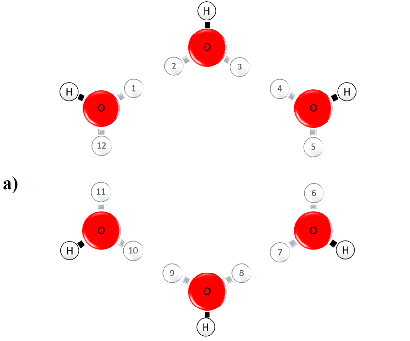
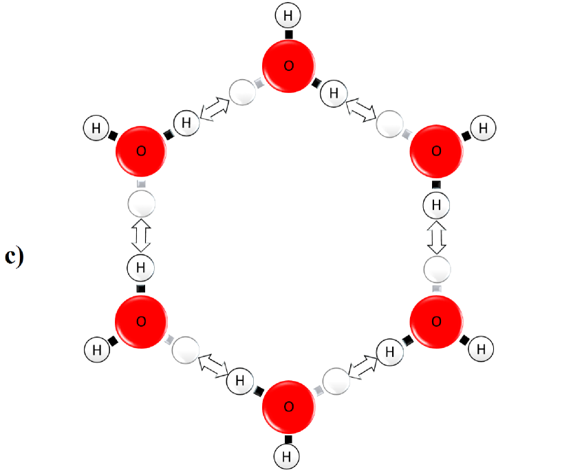
Figure 1: (a) The hexagonal lattice. It is made of OH^- ions in fixed positions relative to each other. Edges can be interpreted as H-bonds. Protons are allowed to live on the enumerated locations. Ice rules are satisfied only by $2$ of the six-proton configurations given in (b) and (c). Transitions between them require simultaneous relocations of the six protons within the ring in the directions depicted by two-sided arrows. Any other configuration accessible from (b) or (c) by successive proton relocations in H-bonds is called an ionic defect. Bjerrum defects occur in all the other configurations including the remaining six-proton configurations.

II Model and Methods

Although their unit cells belong to different space groups, the basic structures of both ice I${}_{\text{h}}$ and XI can be visualized as a hexameric box whose planes are either chair-form or boat-form 3-d hexamers. To reduce the complexity, we restrict our model to a 2-d hexagonal ring with a hydroxyl ion (OH^-) resides in each vertex, as shown in figure 1-a. Rigid rotations of the vertices are not taken into account because of the high energy cost assumed in microscopic models 2006_PTInIceIh and predicted in experiments 2015_CorrPTInIceXI . Each edge linking two vertices represents a H-bond and includes two equally likely locations for H⁺ ions. These locations (enumerated in figure 1-a) can be regarded as a crystal lattice in which H⁺ ions, or protons, move according to the Hamiltonian

$$\begin{aligned} H_{H\!ex}=\sum_{j=1}^{12}W_{j}n_{j}-\sum_{j=1}^{12}J_{j,j+1}(a_{j}^{\dagger}a_{j+1}+a_{j}a_{j+1}^{\dagger})+\sum_{j=1}^{12}V_{j,j+1}n_{j}n_{j+1}+\lambda,\end{aligned}$$ (1)

where subscripts are in mod $12$, $n_{j}=a_{j}^{\dagger}a_{j}$ is the proton number operator at lattice site $j$, $a_{j}^{\dagger}$ and $a_{j}$ are respectively proton creation and annihilation operators that obey the following anticommutation relations

$$\{a_{j},a_{k}\}=\{a_{j}^{\dagger},a_{k}^{\dagger}\}=0,\{a_{j},a_{k}^{\dagger}\}=\delta_{jk}.$$ (2)

On-site energy $W_{j}$ can be taken as the total potential felt by a proton at $j$th site, i.e., the sum of a Morse potential describing the single (covalent) bond with the adjacent OH^- ion and a Coulomb potential representing the electrostatic attraction to the opposite OH^- ion. $J_{j,j+1}$ stands for the orbital interactions which causes proton tunneling. Its expected dependence on the geometry implies that $J_{j,j+1}^{(\text{edge})}\gg J_{j,j+1}^{(\text{vertex})}$ where the former is the intermolecular proton tunneling coefficient for the neighbouring sites occupying the same edge, while the latter is the intramolecular proton tunneling coefficient for the successive sites close to the same vertex. As $J_{j,j+1}^{(\text{edge})}$ should already be quite small compared to other coefficients, we can neglect $J_{j,j+1}^{(\text{vertex})}$. This assumption guarantees the absence of any quantum correlation between the quantum tunneling events through individual hydrogen bonds in the isolated hexamer. $V_{j,j+1}$ is introduced to penalize two-proton cases associated with the violation of ice rules. Edge sharing sites and vertex sharing sites have different penalty coefficients as well as different tunneling coefficients. Presence of two protons on the same edge is called as a Bjerrum defect, whereas occupation of both sites near the same vertex is called as an ionic defect. As Bjerrum defects require more energy, $V_{j,j+1}^{(\text{edge})}\gg V_{j,j+1}^{(\text{vertex})}$. Finally, $\lambda$ is a constant responsible for the total intermolecular interactions between vertices, such as Pauli repulsion, Van der Walls interaction, and London dispersion.

Symmetry of the lattice provides that $W_{j}=W$, $J_{j,j+1}^{(\text{edge})}=J$, $V_{j,j+1}^{(\text{edge})}=V_{inter}$, and $V_{j,j+1}^{(\text{vertex})}=V_{intra}$.

So far, we have focused only on nearest-neighbor interactions and neglected the further interactions with other neighbors, including the concerted tunneling of the six protons arising from the collective overlap of the orbitals. The effect of long-range interactions on the proton dynamics in water ice was in fact proposed to be negligible at low temperatures 2006_PTInIceIh . However, unlike long-range intra-ring interactions, the long-range inter-ring interactions are expected to be non-negligible for the single-ring dynamics. The electrostatic and topological interactions with adjacent rings should at least have significant effects on the parameters $W$, $J$, $V_{inter}$, and $V_{intra}$. We assume that the effects of other rings on each of these parameters can be approximated respectively by a single averaged effect. In what follows $W$, $J$, $V_{inter}$, and $V_{intra}$ are recounted as effective parameters that include mean-field averages.

To obtain a pseudo-spin Hamiltonian by preserving the anti-commutation relations (given in equation (2)), we apply the Jordan-Wigner transformation for $a_{j}$, $a_{j}^{\dagger}$, and $n_{j}$ in equation (1) in such a way below

$$\begin{aligned} a_{j}&=\exp\left(-\text{i}\pi\sum_{k=1}^{j-1}\sigma_{-}^{(k)}\sigma_{+}^{(k)}\right)\sigma_{+}^{(j)},\\ a_{j}^{\dagger}&=\exp\left(+\text{i}\pi\sum_{k=1}^{j-1}\sigma_{-}^{(k)}\sigma_{+}^{(k)}\right)\sigma_{-}^{(j)},\\ n_{j}&=\sigma_{-}^{(j)}\sigma_{+}^{(j)},\end{aligned}$$ (3)

where $\sigma_{-}^{(j)}=|1_{j}\rangle\langle 0_{j}|$ and $\sigma_{+}^{(j)}=|0_{j}\rangle\langle 1_{j}|$ with the convention for Pauli $z$ operator that $\sigma_{z}^{(j)}=|0_{j}\rangle\langle 0_{j}|-|1_{j}\rangle\langle 1_{j}|$. Note that in contrast to the standard application of the Jordan-Wigner transformation on electron transport phenomena, the creation of a proton at the $j$th site is an energy lowering process here.

After writing (3) in terms of Pauli operators, i.e., $n_{j}=\frac{1}{2}\left(I^{(j)}-\sigma_{z}^{(j)}\right)$ and $\sigma_{\pm}^{(j)}=\frac{1}{2}\left(\sigma_{x}^{(j)}\pm\text{i}\sigma_{y}^{(j)}\right)$, we substitute it into (1) and arrive at the following pseudo-spin Hamiltonian

$$\begin{aligned} H_{H\!ex}=&+\sum_{j=1}^{6}J_{x}\left(\sigma^{(2j-1)}_{x}\otimes\sigma^{(2j)}_{x}+\sigma^{(2j-1)}_{y}\otimes\sigma^{(2j)}_{y}\right)\\ &+\sum_{j=1}^{6}J_{z}^{(\text{inter})}\left(\sigma^{(2j-1)}_{z}\otimes\sigma^{(2j)}_{z}\right)\\ &+\sum_{j=1}^{6}J_{z}^{(\text{intra})}\left(\sigma^{(2j)}_{z}\otimes\sigma^{(2j+1)}_{z}\right)\\ &+\sum_{j=1}^{12}B\,\sigma^{(j)}_{z}+\tilde{\lambda},\end{aligned}$$ (4)

where the superscripts of the Pauli matrices are in mod $12$, $J_{x}=-J/2$, $J_{z}^{(\text{inter})}=V_{inter}/4$, $J_{z}^{(\text{intra})}=V_{intra}/4$, $B=-(2\,W+V_{inter}+V_{intra})/4$, and $\tilde{\lambda}=\lambda+6\,W+3\,(V_{inter}+V_{intra})/2$. Note that these parameters have some contributions from the mean-field averages of the effects of the surrounding hexamers and the construction of the Hamiltonian guarantees the absence of any quantum correlation between the quantum tunneling events through individual hydrogen bonds in the isolated hexamer. Also note that the same pseudo-spin formalism described above has been recently used in 2018_Pusuluk to investigate the role of proton tunneling in biological catalysis.

The most general quantum state of pseudo-spins can be described using density matrix formalism such that each computational basis state represents a different configuration of protons. For example, configurations in figures 1-b and c are respectively represented by basis states $|010101010101\rangle$ and $|101010101010\rangle$, so that the protons can exist in any coherent (or incoherent) superposition of these states during the dynamical evolution of the closed (or open) system. Suppose that the proton residing at the site $j=2$ in the former configuration moves to the site $j=1$ by either classical hopping or quantum tunneling between the initial and final times $t_{i}$ and $t_{f}$. In the case of thermally activated classical hopping, it leaves the site $j=2$ at $t=t_{i}$, then enters into the exterior space between the sites, and finally reaches the site $j=1$ at $t=t_{f}$. Since we do not take into account its presence in the exterior space between the sites, it disappears at the site $j=2$ at $t=t_{i}$ and reappears at the site $j=1$ at $t=t_{f}$ in our model, i.e., $\rho(t)=|0\rangle\langle 0|$ where $|0\rangle\equiv|000101010101\rangle$ and $t_{i}<t<t_{f}$. Conversely, it will never enter into the exterior space between the sites in the course of its motion during tunneling, but it will be delocalized between both sites, i.e., $\rho(t)=|\psi\rangle\langle\psi|$ where $|\psi\rangle=\alpha|1\rangle+\beta|2\rangle$, $|1\rangle\equiv|100101010101\rangle$, $|2\rangle\equiv|010101010101\rangle$, $|\alpha|^{2}+|\beta|^{2}=1$, and $t_{i}<t<t_{f}$. In this case, it is found at the first site with a probability of $|\alpha|^{2}$ if its location is measured at any time between $t_{i}$ and $t_{f}$. The decoherence taking place at the end of quantum tunneling, at $t=t_{f}$, converts the coherent superposition $|\psi\rangle\langle\psi|$ into incoherent superposition $|\alpha|^{2}|1\rangle\langle 1|+|\beta|^{2}|2\rangle\langle 2|$ removing the off-diagonal elements from the density matrix.

The unidirectional tunneling process described above can be captured by a snapshot of the state within our pseudo-spin formalism, that is to say, we can detect it by evaluating the off-diagonal elements of the pseudo-spin density matrix at a single time. The advantages of our approach go beyond this. Consider the static structures of pseudo-spins, e.g., the ground state during closed-system dynamics or the thermal state during open-system dynamics. When such a stationary state equals to $|\psi\rangle\langle\psi|$, it means that the proton under consideration delocalizes between the first and second sites over a long time period. This can be regarded as a quantum tunneling of the proton back and forth between these two sites since the state never collapses onto the basis states, which represent the proton localizations at their respective sites (see the same usage of the term in 2015_CorrPTInIceXI ; 2011_CorrPTInIceVII ) . In contrast, we cannot claim a back and forth tunneling event when the steady state is found to be $|\alpha|^{2}|1\rangle\langle 1|+|\beta|^{2}|2\rangle\langle 2|$. Hence, in addition to unidirectional proton tunneling events in the short time limit, the bidirectional proton tunneling events in the long time limit are also described by well-defined density matrices.

Mixed states like the incoherent superpositions above cannot be generated from pure initial states during the closed-system dynamics governed by the Hamiltonian (4). But they can be generated from coherent superposition states as a result of environmental decoherence that will be described in what follows.

II.1 Open system dynamics

It is hard to draw a generic model of the environment for the motion of protons through H-bonds. Such a model should include at least three kinds of vibrations as each individual H-bond is defined by three geometric parameters, e.g., length of the proton-donating bond, donor-acceptor separation and bond angle. However, a minimalistic model consisting of just the periodic oscillations associated with the lengths of proton-donating bonds seems to be sufficient to describe the low-temperature dynamics of protons in a hexameric H₂O ring as in the following. These oscillations can be incorporated into our model as independent thermal baths around lattice sites with individual self-Hamiltonians

$$H_{B}^{(j)}=\sum_{k}\hbar\omega_{j,k}\,b_{j,k}^{\dagger}b_{j,k},$$ (5)

where $b_{j,k}^{\dagger}$ and $b_{j,k}$ are phonon creation and annihilation operators associated with the $k$th oscillator mode at the $j$th site. We assume that the equilibrium positions of the protons are linearly coupled to the positions of the phonons through

$$\begin{aligned} H_{I}&=\sum_{j}n_{j}\,\,\,\sum_{k}\,\left(g_{j,k}b_{j,k}^{\dagger}+g^{*}_{j,k}b_{j,k}\right)\\ &\propto\sum_{j}\sigma_{z}^{(j)}\sum_{k}\,\left(g_{j,k}b_{j,k}^{\dagger}+g^{*}_{j,k}b_{j,k}\right).\end{aligned}$$ (6)

It is important to realize that the local interaction described above induces the entanglement of each pseudo-spin with the positions of associated phonons. In the absence of spin-spin coupling ($J_{x}=0$), the dynamics of the pseudo-spins are fully separated from each other, and each pseudo-spin undergoes a pure dephasing process.

Before extending this discussion to the case of non-vanishing inter-spin coupling, let us first examine the role of memory effects in open system dynamics. The Born-Markov approximation can be justified only if the state of pseudo-spins varies over a time scale much longer than the lifetime of the environmental excitations. The vibration of the O$-$H bond in O$-$H$\cdot\cdot\cdot$O systems has a period of $\simeq 10$ fs, which corresponds to a stretch harmonic frequency of $\simeq 3500$ cm^-1. Unlike the short-lived ($\approx 1$ ps) H-bonds in liquid water 2001_HBLifeTime , H-bonds survive sufficiently long in ice I${}_{\text{h}}$ and the jump time of protons in these bonds is larger than tens of fs, e.g., is equal to $3.7$ ps at $5$ K 2009_CorrPTInIceIhAndIc . So, we can describe the picosecond evolution of the pseudo-spins’ state $\rho$ on the basis of a Markovian master equation in the following Lindblad form BreuerAndPetruccione-2002

$$\frac{d\rho}{dt}=-\frac{\text{i}}{\hbar}[H_{H\!ex}+\hbar H_{L\!S},\rho]+\mathcal{D}(\rho),$$ (7)

where the Lamb shift Hamiltonian provides a unitary contribution to the open dynamics and reads

$$H_{L\!S}=\sum_{\omega}\sum_{j,j^{\prime}}S_{jj^{\prime}}(\omega)\,A_{j}^{\dagger}(\omega)\,A_{j^{\prime}}(\omega),$$ (8)

whereas the dissipator is defined by

$$\begin{aligned} \mathcal{D}(\rho)=\sum_{\omega}\sum_{j,j^{\prime}}\gamma_{jj^{\prime}}(\omega)\,\big{(}A_{j^{\prime}}(\omega)\rho A_{j}^{\dagger}(\omega)-\frac{1}{2}\{A_{j}^{\dagger}(\omega)\,A_{j^{\prime}}(\omega),\rho\}\big{)},\end{aligned}$$ (9)

with $\omega=\epsilon_{m}-\epsilon_{m^{\prime}}$. Here, $\epsilon_{m}$’s are the eigenvalues of pseudo-spin Hamiltonian given in (4) and Noise operators $A_{j}(\omega)$ are the eigenoperators of this self-Hamiltonian

$$A_{j}(\omega)=\sum_{\epsilon_{m}-\epsilon_{m^{\prime}}=\omega}|\epsilon_{m^{\prime}}\rangle\langle\epsilon_{m^{\prime}}|A_{\alpha}|\epsilon_{m}\rangle\langle\epsilon_{m}|,$$ (10)

where $A_{j}$ are the Hermitian operators coupled to the environment, i.e., Pauli $z$ operators as introduced in equation (6). Coefficients $S_{jj^{\prime}}(\omega)$ and $\gamma_{jj^{\prime}}(\omega)$ are respectively the imaginary part and half of the real part of the one-sided Fourier transformation of the thermal bath correlation function given by

$$\Gamma_{jj^{\prime}}(\omega)=\frac{1}{\hbar^{2}}\int_{0}^{\infty}ds\,e^{i\,\omega\,s}\left\langle B_{j}^{\dagger}(s)B_{j^{\prime}}(0)\right\rangle_{\text{th}},$$ (11)

where $B_{j}(s)$ are the interaction picture representations of the bath operators (included in (6)) and $J(\omega)$ is the spectral density function encapsulating all the effects of the environment. We assume that each pseudo-spin is associated with an independent environment, $\Gamma_{jj^{\prime}}=\Gamma_{jj}\,\delta_{jj^{\prime}}$. Furthermore, we focus on a symmetric lattice at a constant temperature $T$ that makes these individual baths identical, so $\Gamma_{jj}=\Gamma$.

The normal modes of lattice vibrations are more complicated in real water ice. The lattice sites, especially the pair of sites sharing the same vertex, are so close to each other that it is expected to find correlations between them. Presence of the correlations between the individual baths may result in the emergence of quantum correlations between the quantum tunneling events in the course of open system dynamics. However, we would like to restrict our analysis to the importance of classical correlations between the quantum tunneling events on the overall proton mobility. Hence, we ignore the correlations between the individual baths as well as the Hamiltonian parameter $J_{j,j+1}^{(\text{vertex})}$.

II.2 Measures of quantum correlations

Quantum coherence is the degree of quantum superposition found in a generic state $\rho$ with respect to a given orthogonal basis $\{|m\rangle\}$. One of the most widely used measures that satisfy all the requirements for a proper measure of quantum coherence is the $l_{1}$ norm of coherence Plenio-2014 , defined as

$$C_{l_{1}}\!\left[\rho\right]=\sum_{m\neq m^{\prime}}|\langle m|\rho|m^{\prime}\rangle|.$$ (12)

Off-diagonal elements of the density matrix $\rho$ are related to the transitions between computational basis states, and each basis state represents a different configuration of the protons in our model. Hence, the $l_{1}$ norm of the pseudo-spins’ state quantifies the quantum coherent proton mobility when the proton number is fixed. As an example, $|m\rangle$ equals to $|b\rangle\equiv|01\rangle^{\bigotimes 6}$ and $|c\rangle\equiv|10\rangle^{\bigotimes 6}$ for the configurations respectively depicted in figures 1-b and c. A transition from one of these states to the other requires simultaneous relocations of the six protons to their adjacent empty sites in H-bonds. Any quantum coherent superposition $|\psi\rangle=\alpha|b\rangle+\beta|c\rangle$ with $|\alpha|^{2}+|\beta|^{2}=1$ represents such a motion if it takes place in the form of concerted tunneling of six protons between the corresponding configurations. The extent of the quantum character of this motion of the protons is reflected in the density matrix by the off-diagonal elements $\langle b|\rho|c\rangle=\alpha\beta^{*}$ and $\langle c|\rho|b\rangle=\alpha^{*}\beta$. The sum of the absolute values of these elements is maximum when $\alpha=\beta=1/\sqrt{2}$, and this corresponds to a quantum state in which the protons can be found in each of the two configurations with a probability of $1/2$ if their locations are measured.

Another proper measure of coherence is the relative entropy of coherence Plenio-2014 :

$$C_{R}^{\mathrm{IC}}\!\left[\rho\right]=\min_{\varsigma\in\mathrm{IC}}\left(S\left[\rho||\varsigma\right]\right)=S[\rho_{d}]-S[\rho],$$ (13)

where the minimum is taken over the set of incoherent states (IC) that are diagonal in the basis $\{|m\rangle\}$, $S\left[\rho||\varsigma\right]$ is the quantum relative entropy that equals to $-\mathrm{tr}\!\left[\rho\,\left(\log_{2}\rho-\log_{2}\varsigma\right)\right]$, $S[\rho]$ is the von Neumann entropy that equals to $-\mathrm{tr}\!\left[\rho\,\log_{2}\rho\right]$, and $\rho_{d}$ is the diagonal part of the density matrix $\rho$. That is to say, $C_{R}^{\mathrm{IC}}\!\left[\rho\right]$ measures the distinguishability of a density matrix with a modified copy in which the off-diagonal elements are removed by a full dephasing process. Whereas $C_{l_{1}}\!\left[\rho\right]$ takes into account distinct tunneling pathways independently of each other, $C_{R}^{\mathrm{IC}}\!\left[\rho\right]$ does not discriminate between these pathways that rearrange the proton configuration and highlights the overall nonclassical mobility, hence showing a holistic picture.

Quantum correlations also arises from the superposition principle. Nonlocal correlations found in nonseparable quantum superposition states are known as quantum entanglement. Entanglement of formation Wooters-1996 is a good measure of entanglement for a generic bipartite state $\rho$ and is defined as

$$E_{F}\!\left[\rho\right]=\min\left(\sum_{i}\mathrm{Q}^{(i)}E_{E}\!\left[|\psi_{i}\rangle\langle\psi_{i}|\right]\right),$$ (14)

where the minimum is taken over all the possible pure state decompositions that realize $\rho=\sum_{i}\mathrm{Q}^{(i)}|\psi_{i}\rangle\langle\psi_{i}|$, and $E_{E}$ is the entropy of entanglement, the unique measure of entanglement for pure bipartite states that equals to the von Neumann entropy of the reduced state of one of the two subsystems, i.e., $E_{E}[\rho]=S[\rho_{1(2)}]=(S\circ\mathrm{tr}_{2(1)})[\rho]$. Although it is hard to compute $E_{F}\!\left[\rho\right]$ for a general state, even numerically, an explicit formula in the form of a binary entropy can be derived in the case of two-qubit systems:

$$E_{F}\!\left[\rho\right]=-f\log_{2}(f)-(1-f)\log_{2}(1-f),$$ (15)

where $f=f(C)=(1+\sqrt{1-C^{2}})/2$ and $C$ is an entanglement monotone, called concurrence Wooters-2000 . This entanglement monotone is defined as

$$C[\rho]=\max\left(0,\sqrt{\lambda_{1}}-\sqrt{\lambda_{2}}-\sqrt{\lambda_{3}}-\sqrt{\lambda_{4}}\right),$$ (16)

where $\lambda_{i}$ are the eigenvalues of the operator $\rho(\sigma_{y}\otimes\sigma_{y})\,\rho^{\ast}(\sigma_{y}\otimes\sigma_{y})$ in decreasing order. In addition to providing an explicit formula for the entanglement of formation, the concurrence can also be used to reveal one of the most fundamental properties of entanglement known as the monogamy of entanglement Wooters-2000 , which imposes a trade-off between the amount of entanglement between different subsystems in a composite system.

As each edge in figure 1-a represents a H-bond, the entanglement of formation of the reduced state of pseudo-spins lying on the same edge quantifies the entanglement generated by proton tunneling through the corresponding H-bond. Besides this, non-zero entanglement of formation between a pseudo-spin pair lying on different edges indicates the inter-bond entanglement between the protons that belong to corresponding H-bonds. The trade-off between intra-bond and inter-bond entanglements can then be investigated using the concurrence. However, quantum correlations are not limited to quantum entanglement, e.g., separable mixed states can possess nonclassical correlations known as quantum discord Vedral-2001 ; Zurek-2002 when the orthogonality condition on local bases breaks down at least in one subsystem and provides local indistinguishability. The original definition of quantum discord Zurek-2002 is grounded in the difference between two different quantum generalizations of mutual information:

$$\begin{aligned} \delta_{1:2}&=I[\rho]-J[\rho]\equiv\left(-S[\rho]+S[\rho_{1}]+S[\rho_{2}]\right)-\max_{\{M_{i}^{(2)}\}}\left(S[\rho_{1}]-S[\rho_{1}|\{M_{i}^{(2)}\}]\right)\\ &=\min_{\{M_{i}^{(2)}\}}\left(S[\rho_{2}]+\sum_{i}\mathrm{P}_{i}S[\rho_{1|M_{i}^{(2)}}]-S[\rho]\right),\end{aligned}$$ (17)

where $S[\rho_{1}|\{M_{i}^{(2)}\}]$ is the quantum conditional entropy of the first subsystem, given the complete measurement $\{M_{i}^{(2)}\}$ on the second subsystem and $\rho_{1|M_{i}^{(2)}}=\mathrm{tr}_{2}[M_{i}\,\rho\,M_{i}^{\dagger}]/\mathrm{P}_{i}$ are post-measurement states of the first subsystem with corresponding probabilities $\mathrm{P}_{i}=\mathrm{tr}_{2}[M_{i}^{\dagger}\,M_{i}\,\rho]$.

Quantum discord is the measure of nonclassical correlations which includes entanglement as a subset since the first quantum generalization of mutual information measures the total correlations between subsystems, whereas the second generalization $J[\rho]$ quantifies only classical correlations Vedral-2001 . In other words, quantum information theory can describe all correlations contained in a complex system in a rigorous way. Classical correlations generated by classical proton hopping through a H-bond can be quantified by the mutual information $J$ between the pseudo-spins lying on the edge corresponding to this bond. Moreover, classical correlations between a pair of protons that belong to different H-bonds in the H₂O hexamer can be captured by $J[\rho_{jj^{\prime}}]$ where $\rho_{jj^{\prime}}$ is the reduced state of pseudo-spins $j$ and $j^{\prime}$ that lie on the edges corresponding to these H-bonds. Note that the classical motion of protons does not appear during the closed system dynamics in our model, but arises from the interaction with the environment.

Since any analytic expression is unknown for the mutual information based measure $\delta_{1:2}$ in a generic system, it is hard to evaluate it. However, an explicit formula of a distance-based measure known as the geometric measure of discord Vedral-2010 is available for a generic two-qubit system which can be written in the Bloch representation:

$$\begin{aligned} \rho&=\frac{1}{4}\Big{(}\mathbb{I}_{1}\otimes\mathbb{I}_{2}+\sum_{i=1}^{3}x_{i}\,\mathbb{I}_{1}\otimes\sigma_{i}^{(2)}+\sum_{i=1}^{3}y_{i}\,\sigma_{i}^{(1)}\otimes\mathbb{I}_{2}+\sum_{i,i^{\prime}=1}^{3}T_{ii^{\prime}}\,\sigma_{i}^{(1)}\otimes\sigma_{i^{\prime}}^{(2)}\Big{)}\end{aligned}$$ (18)

where $\sigma_{i}$ stands for the Pauli sigma matrices. Using this representation, the geometric measure of discord can be calculated as:

$$D_{G,1:2}^{\mathrm{ZD}}=\frac{1}{4}\left(\|\vec{x}\|^{2}+\|T\|^{2}-k_{max}\right),$$ (19)

where $\vec{x}$ equals to $(x_{1},x_{2},x_{3})$ with $x_{i}=\mathrm{tr}[\rho(\mathbb{I}_{1}\otimes\sigma_{i}^{(2)})]$, $\|T\|^{2}=\mathrm{tr}[T^{T}T]$ with $T=T_{ii^{\prime}}\,|i\rangle\langle i^{\prime}|$, $k_{max}$ is the largest eigenvalue of the matrix $K=\vec{x}\,\vec{x}^{T}+T^{T}T$. This measure actually minimizes the distance of a given state $\rho$ to the set of states with zero discord (ZD) using the metric squared Hilbert-Schmidt norm, $\|\rho-\rho^{\prime}\|^{2}=\mathrm{tr}[\rho-\rho^{\prime}]^{2}$.

III Implementation of the model

Almost all of the parameters of the pseudo-spin Hamiltonian (4) except $J_{x}$ can be determined using the tools of quantum chemistry by taking into account all the details of the electronic structure of water ice, e.g. performing a number of different ab initio density functional calculations for some of the possible $2^{12}$ proton configurations. It is also possible to construct a realistic spectral density function based on the molecular dynamics simulations or the density functional theory calculations. However, this would not only increase the demand for computational cost of our model, but also reduce its explanatory power since the model parameters are assumed to have contributions from the mean-field averages of the effects of the surrounding hexamers. On the contrary, the present work aims to construct a simple and physically insightful model with the minimum number of parameters that can be estimated from comparisons of the predictions of the model with experimental results. In what follows we show that the steady state of the equation (7) depends on only two parameters in contrast to previous multi-parameter models and the quantum information theoretic analysis of this state is enough to give a quantitative description of the experimental data.

III.1 Extension to the physical system

Before elaborating on the final steady state of the equation (7), we first find a reasonable map between the actual 3-d structures of water ice and the present 2-d model of a single hexamer. If we extended the model by connecting multiple hexamers in 3-d as in the water ice, we would first replace OH^- ions with O atoms in the vertices and increase the number of equally likely locations for protons close to each vertex from two to four, i.e., the local constraints on a single hexamer would change. Keeping this difference in mind, we infer the ordering dynamics in multi-hexamer real structures from the underlying proton dynamics in single hexamers and construct the map between the model and physical system based on the single-hexamer proton relocation events occurring in them.

Both of the ice I${}_{\text{h}}$ and XI obey the ice rules. However hexagonal rings of ice XI possess a global proton order which is absent in ice I${}_{\text{h}}$, i.e., H₂O hexamers sharing the same 3-d form and the same orientation have also the same proton configuration. This proton order can’t be preserved in the presence of proton relocation unless each of these hexamers simultaneously switches into another proton configuration through a collective motion of the six protons. Thus, not only each of the 3-d hexamers, but also the whole ice XI crystal being constituted by them is allowed to be found only in two different configurations. The switch between these two configurations can be mapped to the transition between $|01\rangle^{\bigotimes 6}$ and $|10\rangle^{\bigotimes 6}$ pseudo-spin states (respectively depicted in figures 1-b and c) as both of them require concerted six-proton relocation.

$|01\rangle^{\bigotimes 6}$ and $|10\rangle^{\bigotimes 6}$ pseudo-spin states span the whole subspace in which the single hexamer satisfies the ice rules. In a sense, we assume that this ice rule preserving subspace in the model corresponds to the proton-ordered phase in hexagonal water ice.

Ice I${}_{\text{h}}$ is composed of 3-d hexamers that also fulfill the ice rules but do not show global correlation. Proton configuration of these hexamers can be achieved from the ones in ice XI by the proton relocation events occurring through H-bonds and keeping the proton number in each hexamer fixed at six. In our model, similar proton relocation events bring the states living inside the ice rule preserving subspace into another subspace spanned by 62 pseudo-spins representing the ionic defects. Thus, this defective pseudo-spin subspace can be assumed to coincide with the proton-disordered phase in hexagonal water ice.

III.2 Asymptotic limit of the model

Here and in the following, we consider the steady state solution of the equation (7). The chosen interaction with the environment does not bring the system into a thermal equilibrium in general. On the contrary, it divides $2^{12}$-dimensional Hilbert space $\mathcal{H}$ into subspaces $\mathcal{H}_{\mathcal{J}}$ each of which is independently invariant under $\{A_{j}\}_{j=1}^{12}$ operators. In the asymptotic limit, it provides a detailed balance only inside these subspaces as below:

$$\begin{aligned} \rho_{\infty}&=\sum_{\mathcal{J}}\frac{\mathrm{P}\left(\mathcal{J}\right)}{\mathcal{Z}\left(\mathcal{J}\right)}\sum_{|\epsilon_{m}\rangle\in\mathcal{H}_{\mathcal{J}}}e^{-\beta\epsilon_{m}}|\epsilon_{m}\rangle\langle\epsilon_{m}|,\end{aligned}$$ (20)

where

$$\mathrm{P}\left(\mathcal{J}\right)=\sum_{|\epsilon_{m}\rangle\in\mathcal{H}_{\mathcal{J}}}\langle\epsilon_{m}|\,\rho(t=0)|\epsilon_{m}\rangle,$$ (21)

and

$$\mathcal{Z}\left(\mathcal{J}\right)=\sum_{|\epsilon_{m}\rangle\in\mathcal{H}_{\mathcal{J}}}e^{-\beta\epsilon_{m}},$$ (22)

with $\beta=1/k_{B}T$.

One of the subspaces $\mathcal{H}_{\mathcal{J}}$ consists of two special kinds of pseudo-spin states mentioned in the previous subsection, i.e., 2 pseudo-spin states obeying the ice rules and 62 pseudo-spin states corresponding to ionic defects. As these state sets are assumed to map to the proton-ordered and disordered phases of the hexagonal water ice respectively, we label their union by $\mathcal{H}_{ice}$. If the initial state $\rho(t=0)$ lives only in this $64$-dimensional subspace, the state of the pseudo-spins that relax to equilibrium still stays inside the same subspace as follows

$$\begin{aligned} \rho_{\infty}^{ice}&=\sum_{|\epsilon_{m}\rangle\in\mathcal{H}_{ice}}e^{-\beta\epsilon_{m}}|\epsilon_{m}\rangle\langle\epsilon_{m}|\quad/\sum_{|\epsilon_{m}\rangle\in\mathcal{H}_{ice}}e^{-\beta\epsilon_{m}}.\end{aligned}$$ (23)

It is straightforward to show that the athermal attractor above essentially depends on two free parameters, $J_{x}$ and $J_{z}^{(\text{intra})}$ as all the energy eigenvalues of subspace $\mathcal{H}_{ice}$ have a common functional dependence on the remaining coefficients included in (4).

III.3 Characterization of proton ordering/disordering

A temperature dependent transition between two different phases can be characterized by the presence of two different steady states above and below the phase transition temperature. Although our master equation has a unique steady state solution denoted by $\rho_{\infty}^{ice}(T)$, it shows different features above and below the phase transition temperature range which are reflected by i) $P_{BF}(T)$, the probability of pseudo-spins to be found inside the ice-rule preserving subspace and ii) $S[\rho_{\infty}^{ice}(T)]$, the von Neumann entropy of pseudo-spins.

In our model, each basis state represents a different configuration of the protons. As explained in section III.1, the 2-dimensional ice rule preserving subspace spanned by $\{|01\rangle^{\bigotimes 6},|10\rangle^{\bigotimes 6}\}$ can be mapped to the XI phase of water ice based on the proton relocation dynamics. Thus, the change in probability $P_{BF}(T)$ can be used as an indicator of the proton-disordering phase transition, e.g., it should be close to unity in XI phase and show a decrease during the transition to I${}_{\text{h}}$ phase.

Presence of unit probability below the phase transition temperature range means that only $4$ particular elements of $\rho_{\infty}^{ice}(T)$ can be nonzero. No matter how small a deviation from unity in $P_{BF}(T)$ is, $64\times 64-4=4092$ more elements of $\rho_{\infty}^{ice}(T)$ can take a non-zero value. This corresponds to an enlargement in the dimension of the effective Hilbert space from $2$ to $64$, which allows the violation of ice rules that was mapped to the proton-disordered phase in section III.1. Hence, there is no need to a significant decline in $P_{BF}(T)$ within the phase transition temperature range to indicate the proton-ordered/disordered transition, but it is sufficient for it to gradually deviate from unity which means a turning point behavior. When it shows a sharp decline above the phase transition temperature range, we have effectively two different steady states above and below the range, each of which has different numbers of non-zero elements and lives in a different Hilbert space.

The von Neumann entropy measures the amount of disorder, uncertainty, or unpredictability of a generic quantum state. Furthermore, each basis state of pseudo-spins represents a different proton configuration in our model. Thus, $S[\rho_{\infty}^{ice}(T)]$ directly quantifies the proton-disorder.

IV Results

IV.1 Model parameters

The values of the parameters used here were estimated from comparisons of the predictions of the model with the previous experiments carried out on the ice I${}_{\text{h}}$/XI transition. Actually, it isn’t easy to observe this transition as protons are expected to become classically immobile around $100-110$ K where a glass transformation occurs 2015_HexPhaseTransition ; 1988_GlassTrans ; 1997_GlassTrans . First calorimetric measurements 1982_KOH-doped ; 1984_KOH-doped overcame this problem by using alkali hydroxides as catalyzer and catched the transition at $72$ K. According to recent complex dielectric constant measurements of pure water ice reported in 2015_HexPhaseTransition , hexagonal ice undergoes a phase transition from proton-disordered ice I${}_{\text{h}}$ to proton-ordered ice XI at $58.9$ K, whereas a reverse transformation occurs at $73.4$ K. Since a charge movement should increase the imaginary part of the dielectric constant $\varepsilon^{\prime\prime}$, these phase transitions were determined by detecting the anomalies in the cooling and warming curves of $\varepsilon^{\prime\prime}(T)$. Whereas a clear peak was observed in the warming curve of $d\varepsilon^{\prime\prime}/dT$ at $73.4$ K, a discontinuous change occurred in the slope of cooling curve of $d\varepsilon^{\prime\prime}/dT$ at $58.9$ K. The former was reflected in the warming curve of $\varepsilon^{\prime\prime}(T)$ as a continuous increase followed by a change in the slope, while the latter corresponded to a smooth change in the slope of the cooling curve of $\varepsilon^{\prime\prime}(T)$. See figure 3 in reference 2015_HexPhaseTransition for more details.

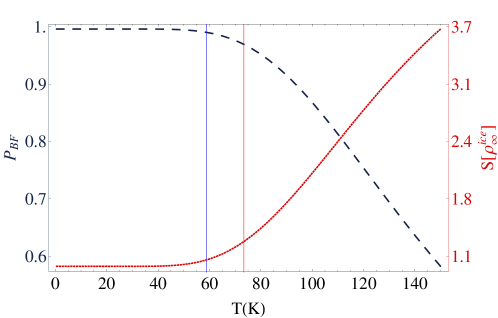
Figure 2: Estimation of the parameters based on the predictions of the model with experiments. XI$\rightarrow$I${}_{\text{h}}$ and I${}_{\text{h}}$$\rightarrow$XI phase transitions of hexagonal ice respectively occur at $58.9$ K and $73.4$ K 2015_HexPhaseTransition . Vertical solid lines coloured blue and red pinpoint these temperatures. The dashed dark blue curve is $P_{BF}(T)$, the probability of pseudo-spins to be found inside the ice rule preserving subspace spanned by $\{|01\rangle^{\bigotimes 6},|10\rangle^{\bigotimes 6}\}$ when they are prepared in the steady state $\rho_{\infty}^{ice}$. We set $J_{x}$ and $J_{z}^{(\text{intra})}$ respectively to $-0.5$ meV and $+10$ meV to observe the violation of ice rules around the phase transition temperatures. The dashed dark red curve shows the temperature dependence of the von Neumann entropy of $\rho_{\infty}^{ice}$.

As opposed to experimental data on $\varepsilon^{\prime\prime}(T)$, no hysteresis is expected between the warming and cooling curves of $P_{BF}(T)$ since we focus on the steady state solution of the master equation and do not allow the system under consideration to be driven out of equilibrium due to quantum fluctuations. Moreover, as our model is restricted to a single hexamer, a sharp discontinuity in $P_{BF}(T)$ is unlikely to occur during phase transition. Hence, instead of a first order phase transition, we anticipate observing a smooth change in the slope of $P_{BF}(T)$ similar to that of the cooling curve of $\varepsilon^{\prime\prime}(T)$ shown in figure 3-a in 2015_HexPhaseTransition and in figure 2 in 2015_CorrPTInIceXI . However, even this smooth change in our finite size system can be treated as evidence of a proton-disordering phase transition since it reflects the true microscopic mechanism driving the proton-disordering process (see sections III.1 and III.3 for details).

Figure 3: First derivative of the free energy with respect to temperature. Since we do not consider any change in the locations of OH^- ions with temperature, we do not include a pressure-volume term in the free energy, i.e., $F=U-k_{B}TS$, where $S$ is the von Neumann entropy.

In this respect, we fixed our free parameters $J_{x}$ and $J_{z}^{(\text{intra})}$ respectively to $-0.5$ meV and $+10$ meV to reproduce the expected trend of $P_{BF}(T)$ using the steady state $\rho_{\infty}^{ice}$ as shown in figure 2. The state of pseudo-spins stays inside the ice rule preserving subspace with a unit probability while $T<58.9$ K. The states outside this subspace violate the ice rules and gradually become available between the blue and red lines. Above the temperature of $\approx 73.4$, $P_{BF}(T)$ shows a sharp decline that corresponds to an ever-increasing population of ice rule violating states. Details of the procedure used in this parameter estimation are given in section VIII.1 in the Electronic Supplementary Material (ESM).

The behaviour of the von Neumann entropy of $\rho_{\infty}^{ice}(T)$ supports the arguments above for the fixed values of $J_{x}$ and $J_{z}^{(\text{intra})}$. According to figure 2, it remains at unity until $58.9$ K. Note that the pseudo-spins live inside the subspace spanned by $\{|01\rangle^{\bigotimes 6},|10\rangle^{\bigotimes 6}\}$ in the same temperature range. Then this unit disorder is possible only if the pseudo-spins can exist in only two orthogonal states living inside this subspace with an equal probability, i.e., the configurations given in figures 1-b and c or two of their coherent superpositions orthogonal to each other are equally likely for the protons. $S[\rho_{\infty}^{ice}(T)]$ rises slowly with further increases of temperature until $73.4$ K. Hence, a smooth change occurs in the proton-disorder around $58.9-73.4$ K. After that, the slope of $S[\rho_{\infty}^{ice}(T)]$ is approximately constant, which shows a rapid increase in the proton disorder. Note that the first derivative of free energy of $\rho_{\infty}^{ice}(T)$ has the same temperature dependence with $P_{BF}(T)$ and $S[\rho_{\infty}^{ice}(T)]$ as shown in figure 3.

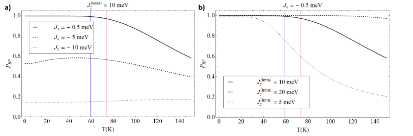
Figure 4: Sensitivity of the behaviour of probability $P_{BF}(T)$ to the fixed values of free parameters $J_{x}$ (a) and $J_{z}^{(\text{intra})}$ (b).

Estimation of the free parameters may still look arbitrary at first glance. However, if we decrease the value of $J_{x}$, $P_{BF}(T)$ cannot get close to unity at any temperature (figure 4-a), which means that the ice rules are always violated and the system can never end up in XI phase. On the contrary, a change in the value of $J_{z}^{(\text{intra})}$ sets the temperature at which the ice rules begin to be violated, apart from the experimentally determined phase transition temperatures (figure 4-b). Hence, the expected temperature dependence of $P_{BF}$ exhibits a sensitivity to our free parameters, i.e., deviations from the fixed values of either $J_{x}$ or $J_{z}^{(\text{intra})}$ that are much smaller than the energy of a H-bond rule out any prediction, preventing the appearance of a slow decline in $P_{BF}(T)$ from unity around $58.9-73.4$ K. Also, this behaviour cannot reappear when the second parameter is also allowed to deviate from its fixed value at the same time. Please see section VIII.2 in the Electronic Supplementary Material (ESM) for the details.

Note that the values of $J_{x}=-0.5$ meV and $J_{z}^{(\text{intra})}=+10$ meV are fixed in this way, and do not only stand for the bare coefficients of a single hexamer but also have contributions from the mean-field averages of the effects of the surrounding hexamers.

IV.2 Quantum aspects of the proton mobility

We summarized several theoretical and experimental findings suggesting the likelihood of proton tunneling in hexagonal water ice in section I. Here, we address two of them using the tools of quantum information theory described in section II.2.

The first claim concerns the role of proton tunneling in I${}_{\text{h}}$/XI phase transition. In reference 2006_PTInIceIh , the motion of the protons was first mapped into a pseudo-spin model, as we do, but then converted to a gauge theory problem. This description allowed the authors to characterize the ordered and disordered phases respectively by confined and deconfined behaviours of ionic defects in the ground state of the system. It was then found that the phase transition under consideration is possible only if the protons tunnel through H-bonds with a rate greater than a critical value (see figure 6-b in 2006_PTInIceIh ). Since the protons are expected to become classically immobile around $100-110$ K where a glass transformation occurs 2015_HexPhaseTransition ; 1988_GlassTrans ; 1997_GlassTrans , this is a reasonable claim. Our predictions shown in figure 4-a suggest that it may be also unlikely for the hexagonal water ice to end up in XI phase unless the tunneling rate is less than another critical value. Thus, further investigation of the quantum aspects of the proton mobility in I${}_{\text{h}}$/XI transition using quantum information theory may yield new knowledge about this topic.

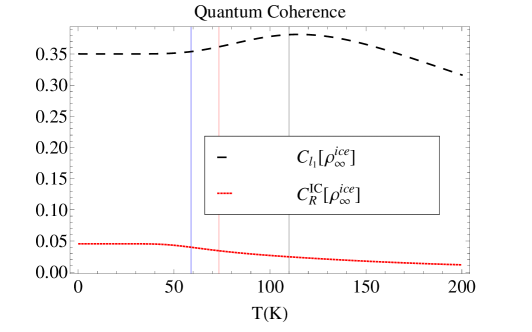
Figure 5: Coherent quantum effects on proton mobility in a H₂O hexamer. Vertical solid lines coloured blue and red indicate the phase transition temperatures 2015_HexPhaseTransition , whereas the vertical black line is anchored to the temperature of the glass transition at which proton mobility is expected to diminish 2015_HexPhaseTransition ; 1988_GlassTrans ; 1997_GlassTrans .

The second claim that will be addressed here is the presence of concerted six-proton tunneling at low temperatures in XI phase. Dielectric constant measurements that determined the phase transition temperatures in pure water ice 2015_HexPhaseTransition were extended down to $5$ K in reference 2015_CorrPTInIceXI , and an anomaly was observed in the cooling and warming curves of $\varepsilon^{\prime\prime}(T)$ in the form of a minimum around $20$ K. The monotonic behaviour of the real part of the dielectric constant observed in the same data and disappearance of the anomaly in the repeat measurements on heavy ice were explained by the back and forth tunneling of protons in groups of six. As mentioned before, the unit disorder of $\rho_{\infty}^{ice}$ at low temperatures (figure 2) may indicate the presence of two equally likely superpositions of the configurations given in figures 1-b and c. Also, each such superposition represents the correlated tunneling of six protons, and quantum information theory is able to study the nature and extent of this correlation (see section II.2).

To provide a first insight into the quantum aspects of proton mobility in a hexameric H₂O loop, we apply the $l_{1}$ norm and relative entropy of coherence on $\rho_{\infty}^{ice}$ as shown in figure 5. $C_{R}^{\mathrm{IC}}\![\rho_{\infty}^{ice}]$, which quantifies the distinguishability of $\rho_{\infty}^{ice}$ from its completely decohered version, remains constant throughout the XI phase and steadily decreases with increasing temperature. Hence, there is a rise in the loss of collective quantumness in the global proton mobility starting with the transition from XI phase to I${}_{\text{h}}$ phase which lasts thereafter. Conversely, $C_{l_{1}}\![\rho_{\infty}^{ice}]$, which is the sum of quantum coherences in individual transitions between proton configuration pairs, shows a different behaviour with respect to temperature. It increases with the XI$\rightarrow$I${}_{\text{h}}$ phase transition and reaches a peak around glass transition. Actually, this behaviour seems to be consistent with the experimental data related to real proton mobility, which indicates a local maximum between $60-110$ K (see figure 3-a in 2015_HexPhaseTransition and figure 2 in 2015_CorrPTInIceXI ) at where the protons are expected to be classically immobile.

The deviation of the temperature dependence of $C_{l_{1}}\![\rho_{\infty}^{ice}]$ from the experimental data below $60$ K is related to the finite size of our model. Although the increase in $\varepsilon^{\prime\prime}(T)$ during the cooling from $20$ K to $5$ K arises from the increasing number of protons involved in the correlated six-proton tunneling events 2015_CorrPTInIceXI , our results are limited to a single hexamer including only six protons. The loss of similarity between the curves of $C_{l_{1}}\![\rho_{\infty}^{ice}(T)]$ and $\varepsilon^{\prime\prime}(T)$ above $110$ K also originates from the restrictions on our model. The rise in $\varepsilon^{\prime\prime}(T)$ after the glass transition 2015_CorrPTInIceXI ; 2015_HexPhaseTransition is likely stem from thermally activated proton hopping, which is expected to suppress quantum coherent proton mobility at these temperatures but outside our scope. Note that the classical motion of the protons enters into our model in the form of incoherent superpositions of pseudo-spins that are generated from coherent superpositions as a result of decoherence.

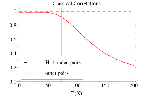
Figure 6: Pairwise classical correlations. The dashed black curve corresponds to the correlations in a single H-bond. Correlations between two protons, each of which belongs to a different H-bond, is shown by the dashed dark red curve.

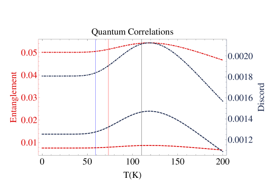
Figure 7: Pairwise quantum correlations in a single H-bond. There is no quantum correlation found between proton pairs belonging to different H-bonds. The dot-dashed dark red curve is the concurrence between pseudo-spins lying on the same edge, while the dashed red curve is the entanglement of formation between them. Their quantum correlations beyond entanglement are measured by quantum discord and its geometric measure, which are displayed respectively as dot-dashed and dashed dark blue curves.

On the other hand, the uptick in $C_{l_{1}}\![\rho_{\infty}^{ice}]$ between the blue and red solid lines in figure 5 offers fresh insights about the importance of coherent proton mobility on the proton ordering dynamics 2006_PTInIceIh , i.e., although the tunneling coefficient is fixed initially, there is an increase in the amount of coherence generated by tunneling events during the phase transition from proton-disordered ice I${}_{\text{h}}$ to proton-ordered ice XI. Also, pinning of $C_{l_{1}}\![\rho_{\infty}^{ice}(T)]$ at a nonzero value below $60$ K eliminates the possibility that the pseudo-spins exist in a maximal mixture of the basis states $|01\rangle^{\bigotimes 6}$ and $|10\rangle^{\bigotimes 6}$. Hence, the presence of unit disorder below $60$ K in figure 4-a should come from a maximal mixture of two orthogonal superpositions of these basis states, i.e., $\rho_{\infty}^{ice}=1/2|\psi_{+}\rangle\langle\psi_{+}|+1/2|\psi_{-}\rangle\langle\psi_{-}|$ where $|\psi_{\pm}\rangle$ are two coherent superpositions such as $\left(|01\rangle^{\bigotimes 6}\pm|10\rangle^{\bigotimes 6}\right)/\sqrt{2}$. Note that each of the superposition states involved in this mixture can be interpreted as a concerted tunneling of six protons back and forth between the configurations represented by the states $|01\rangle^{\bigotimes 6}$ and $|10\rangle^{\bigotimes 6}$. This observation is in accordance with the dielectric anomaly measured in the form of a minimum around $20$ K 2015_CorrPTInIceXI where we suspect a concerted quantum tunneling of six protons could be occurring in each hexamer.

A deeper understanding of the overall behaviour of $C_{l_{1}}\![\rho_{\infty}^{ice}(T)]$ requires investigation of the classical and quantum correlations between pseudo-spin pairs respectively shown in figures 6 and -7. Only classical correlations appear between the pseudo-spins lying on different edges according to these figures. This is actually what we expect to see as we prevent the formation of quantum correlations between these pseudo-spin pairs by setting the Hamiltonian parameter $J_{j,j+1}^{(\text{vertex})}$ to zero and taking the O$-$H stretch vibrations as independent from each other. What is unexpected about these results is that the probability change observed in figure 2 resembles the temperature-dependent behaviour of the classical correlations in figure 6, where the mutual information $J$ of the reduced state of the corresponding pseudo-spins is constant around unity throughout the XI phase and starts falling down during the XI/I${}_{\text{h}}$ transition. This means that there is an approximately maximal amount of classical correlations between the motions of two different protons that belong to different H-bonds below $60$ K.

Beside this, classical correlations between edge sharing pseudo-spins seem to be fixed at unity independent of the temperature. Hence, classical correlations generated by the proton motion in an individual H-bond are invariant under any change in temperature. On the other hand, regardless of the measure that is used to quantify quantum correlations between edge sharing pseudo-spin pairs, quantum correlations generated by proton tunneling through individual H-bonds are found to be quite low. However, each curve in figure 7 shows a similarity with coherent proton dynamics described by $C_{l_{1}}\![\rho_{\infty}^{ice}(T)]$ in figure 5. Thus, although the quantum correlations in H-bonds seem to be insignificant when compared to their classical counterparts, temperature dependence of quantum coherent proton mobility still originates from them.

Based on these observations, we surmise that all the individual proton tunnelings throughout six H-bonds found in a single hexamer become classically correlated at low temperatures. These correlations start to weaken during the phase transition from proton-ordered phase ice XI to proton-disordered phase ice I${}_{\text{h}}$. At the same time, quantum correlations between H-bonded atoms become stronger, reaching a maximum during the glass transition around $110-120$ K.

V Future Directions

The effect of O$-$H stretch vibrations is incorporated into the model in the form of Holstein-type local phonon-proton couplings. Such local interactions can originate from the second quantization of the small site displacements after expanding on-site energies $W_{j}$ around some reference set of coordinates. However, transfer integrals $J_{j,j+1}^{(\text{edge})}$ are also likely to be perturbed by both O$-$H and O$-$O vibrations. Moreover, these perturbations should have a different kind of nature, which can be described by non-local phonon-proton couplings well-known as Peierls-type interaction. Unlike the Holstein-type interaction, this interaction isn’t necessarily destructive and can facilitate proton tunneling between sites. In fact, the fluctuations of the O$-$H and O$-$O bond lengths are expected to have a significant effect on the proton dynamics in real water ice structures. A natural direction to pursue future work is a new quantum master equation approach to open system dynamics of the protons in the presence of both local and non-local phonon couplings. Such a mixed Holstein-Peierls model will reveal the competition between the local and non-local phonon couplings that may be key to understanding this system.

Our first attempts to develop a mixed Holstein-Peierls model using a two qubit model system given in the Electronic Supplementary Material (ESM) show that although nonlocal couplings change the dynamics of the system, the static structure of the final steady state remains same (see section VII). Hence, the bond fluctuations appear not to affect the predictions of the present model unless we do not move on to probe the true proton dynamics around the hexagonal ring in real-time.

The simple pseudo-spin model approach can be readily employed together with the quantum chemical techniques treating electrons and protons quantum mechanically. This additional technique will allow us to give a realistic estimate of both the parameters of the self-Hamiltonian and the form of the spectral density function. It will then be possible to probe the true proton dynamics around the hexagonal ring in real-time. This offers a new opportunity that previous studies didn’t yield. However, our assumptions about the Markovianity of the open system dynamics may not be justified in this case as we will not work in the long-time regime. Thus, this direction also includes description of the proton dynamics using a non-Markovian evolution.

Besides this, our one-qubit pseudo-spin representation of proton locations is suitable to extend the present model to include nuclear spin degrees of freedom, which are usually ignored by the current modelling approaches in the water literature. Actually, the experimentally determined ratio of ortho/para spin states of isolated single water molecules exhibits a temperature dependence which shares similarities with the proton mobility under consideration in this study. In this respect, we are planning to extend the present model to investigate the possible effects of nuclear spins on proton-ordering dynamics in water ice.

VI Conclusion

We constructed a simple pseudo-spin model to investigate both the possibility and the nature of concerted six-proton tunneling in a hexameric H₂O employing the tools of quantum information theory. We demonstrated that the static structure of the final steady state of the chosen master equation depends on only two parameters and the quantum information theoretic analysis of this state is sufficient to give a quantitative description of experimental data.

The role of the external environment on the concerted six-proton tunneling was clearly unveiled as this tunneling process was not imposed by the self-Hamiltonian but emerged naturally in the long-time limit of the low-temperature dynamics of the open system. Thus, phonon-assistance was found to be central in driving the concerted proton tunneling up to the temperature of the phase transition from ice XI to ice I${}_{\text{h}}$. Moreover, it was found to be associated with the emergence of ice rules governing the arrangement of atoms in water ice.

Remaining within the framework of the pseudo-spin model enabled us to approach the correlation problem using the tools of quantum information theory. In turn, we inferred that the $l_{1}$ norm of coherence Plenio-2014 is sufficient to capture the behaviour of coherent proton mobility observed in experiments 2015_HexPhaseTransition ; 2015_CorrPTInIceXI . We also discriminated between quantum and classical correlations in concerted proton tunneling. It was found that the correlations between six proton tunneling events are not inherently quantum in character. Instead, individual tunneling events were allowed to be classically correlated only. Low rates and strong correlations were observed for quantum tunneling events below a critical temperature corresponding to phase transition. Beyond this critical temperature, simulations showed a weakening in the correlations, but an increase in rates. Overall this induces a total increment in the coherent proton mobility until achieving a full proton disorder.

The finding sheds light on the nature of correlations between the individual tunneling events that can’t be addressed by previous studies. This also paves the way to investigating the proton dynamics in real-time to advance our understanding of many-proton tunneling in water ice.

Electronic Supplementary Material
available online at https://dx.doi.org/10.6084/m9.figshare.c.4487114

VII Open System Dynamics of Proton Motion

The state of pseudo-spins lives in a $2^{12}$-dimensional Hilbert space $\mathcal{H}$, that is to say that the density matrix $\rho$ describing this state has $2^{12}\times 2^{12}$ elements. In this respect, it is not straightforward to present the details of its open system dynamics. For the sake of simplicity, and without loss of generality, we will focus on the motion of a single proton between the locations 1 and 2 in the hexamer in what follows (see Fig. 1-a for the details). Hence, instead of working with the twelve-site self-Hamiltonian $H_{H\!ex}$ given in Eq. (1), we will use the following two-site Hamiltonian

$$\begin{aligned} H_{H\!B}&=\sum_{j=1}^{2}W_{j}\,\hat{n}_{j}-J_{12}(a_{1}^{\dagger}a_{2}+a_{1}a_{2}^{\dagger})+V_{12}\,\hat{n}_{1}\hat{n}_{2}+\lambda\,\mathbb{I}_{12}\end{aligned}$$ (S1)

to describe the closed system dynamics. Note that asymmetric version of this Hamiltonian ($W_{1}\neq W_{2}$) was also used in 2018_Pusuluk to investigate the role of proton tunneling in biological catalysis.

After applying the Jordan-Wigner transformation given in Eq. (2) on this two-site Hamiltonian, we end up with the two-qubit Hamiltonian

$$\begin{aligned} H_{H\!B}=J_{x}\left(\sigma^{(1)}_{x}\otimes\sigma^{(2)}_{x}+\sigma^{(1)}_{y}\otimes\sigma^{(2)}_{y}\right)+J_{z}\,\sigma^{(1)}_{z}\otimes\sigma^{(2)}_{z}+B\left(\sigma^{(1)}_{z}+\sigma^{(2)}_{z}\right)+\tilde{\lambda},\end{aligned}$$ (S2)

where $J_{x}=J_{12}/2$, $J_{z}=V_{12}/4$, $B=-(2W+V_{12})/4$, and $\tilde{\lambda}=\lambda+(4W+V_{12})/4$. Eigensystem of this Hamiltonian can be written in an increasing order of the eigenvalues as

$$\begin{cases}e_{1}=-J_{z}+2J_{x}+\tilde{\lambda},&\mbox{}|e_{1}\rangle\mbox{}=(|01\rangle+|10\rangle)/\sqrt{2},\\ e_{2}=-J_{z}-2J_{x}+\tilde{\lambda},&\mbox{}|e_{2}\rangle\mbox{}=(|01\rangle-|10\rangle)/\sqrt{2},\\ e_{3}=-2B+J_{z}+\tilde{\lambda},&\mbox{}|e_{3}\rangle\mbox{}=|11\rangle,\\ e_{4}=+2B+J_{z}+\tilde{\lambda},&\mbox{}|e_{4}\rangle\mbox{}=|00\rangle.\end{cases}$$ (S3)

VII.1 Local proton-phonon coupling

First, we examine the O$-$H stretch vibrations by considering them as two independent thermal baths existing around the proton locations and having the individual self-Hamiltonians $H_{B}^{(j)}$ given in Eq. (5). Also, we will describe the interaction of the proton with these vibrations using the interaction Hamiltonian given in Eq. (6):

$$\begin{aligned} H^{local}_{I}=\sum_{j}\hat{n}_{j}\,\,\,\sum_{k}\,\left(g_{j,k}b_{j,k}^{\dagger}+g^{*}_{j,k}b_{j,k}\right)\propto\sum_{j}\sigma_{z}^{(j)}\sum_{k}\,\left(g_{j,k}b_{j,k}^{\dagger}+g^{*}_{j,k}b_{j,k}\right).\end{aligned}$$ (S4)

VII.1.1 Bath operators in interaction picture

If we switch into the interaction picture, the bath operators $B_{j}=\sum_{k}\,(g_{j,k}b_{j,k}^{\dagger}+g^{*}_{j,k}b_{j,k})$ become

$$\begin{aligned} B_{j}(t)&=e^{X}B_{j}e^{-X}\\ &=B_{j}+[X,B_{j}]+[X,[X,B_{j}]]/2!+[X,[X,[X,B_{j}]]]/3!+...\end{aligned}$$ (S5)

where $X=i\,H_{\mathcal{B}}^{(j)}\,t/\hbar$. To evaluate the commutators above, first we need to find the commutators $[H_{\mathcal{B}}^{(j)},b_{j,k^{\prime}}^{\dagger}]$ and $[H_{\mathcal{B}}^{(j)},b_{j,k^{\prime}}]$. In this respect, the bosonic commutation relations imply that

$$\begin{aligned} [H_{\mathcal{B}}^{(j)},b_{j,k^{\prime}}^{\dagger}]&=\sum_{k}\hbar\omega_{j,k}\,[b_{j,k}^{\dagger}b_{j,k},\,b_{j,k^{\prime}}^{\dagger}]\\ &=\sum_{k}\hbar\omega_{j,k}\,\left(b_{j,k}^{\dagger}[b_{j,k},\,b_{j,k^{\prime}}^{\dagger}]+[b_{j,k}^{\dagger},\,b_{j,k^{\prime}}^{\dagger}]b_{j,k}\right)\\ &=\sum_{k}\hbar\omega_{j,k}\,b_{j,k}^{\dagger}\delta_{k,k^{\prime}}=+\hbar\omega_{j,k^{\prime}}\,b_{j,k^{\prime}}^{\dagger},\end{aligned}$$ (S6)

$$\begin{aligned} [H_{\mathcal{B}}^{(j)},b_{j,k^{\prime}}]&=\sum_{k}\hbar\omega_{j,k}\,[b_{j,k}^{\dagger}b_{j,k},\,b_{j,k^{\prime}}]\\ &=\sum_{k}\hbar\omega_{j,k}\,\left(b_{j,k}^{\dagger}[b_{j,k},\,b_{j,k^{\prime}}]+[b_{j,k}^{\dagger},\,b_{j,k^{\prime}}]b_{j,k}\right)\\ &=\sum_{k}\hbar\omega_{j,k}\,\left(-\delta_{k,k^{\prime}}\right)b_{j,k}=-\hbar\omega_{j,k^{\prime}}\,b_{j,k^{\prime}}.\end{aligned}$$ (S7)

Then, it is easy to calculate the commutators in (S5) after writing them in terms of (S6) and (S7):

$$\begin{aligned} [X,B_{j}]&=(i\,t/\hbar)[H_{\mathcal{B}}^{(j)},B_{j}]\\ &=\sum_{k}(i\,t/\hbar)\left(g^{*}_{j,k}[H_{\mathcal{B}}^{(j)},b_{j,k}]+g_{j,k}[H_{\mathcal{B}}^{(j)},b_{j,k}^{\dagger}]\right)\\ &=\sum_{k}(i\,\omega_{j,k}\,t)\left(-g^{*}_{j,k}b_{j,k}+g_{j,k}b_{j,k}^{\dagger}\right),\end{aligned}$$ (S8)

$$\begin{aligned} [X,[X,B_{j}]]&=(i\,t/\hbar)[H_{\mathcal{B}}^{(j)},[X,B_{j}]]\\ &=\sum_{k}(i^{2}\,\omega_{j,k}\,t^{2}/\hbar)\left(-g^{*}_{j,k}[H_{\mathcal{B}}^{(j)},b_{j,k}]+g_{j,k}[H_{\mathcal{B}}^{(j)},b_{j,k}^{\dagger}]\right)\\ &=\sum_{k}(i^{2}\,\omega_{j,k}^{2}\,t^{2})\left(+g^{*}_{j,k}b_{j,k}+g_{j,k}b_{j,k}^{\dagger}\right),\end{aligned}$$ (S9)

$$\begin{aligned} [X,[X,[X,B_{j}]]]&=(i\,t/\hbar)[H_{\mathcal{B}}^{(j)},[X,[X,B_{j}]]]\\ &=\sum_{k}(i^{3}\,\omega_{j,k}^{2}\,t^{3}/\hbar)\left(+g^{*}_{j,k}[H_{\mathcal{B}}^{(j)},b_{j,k}]+g_{j,k}[H_{\mathcal{B}}^{(j)},b_{j,k}^{\dagger}]\right)\\ &=\sum_{k}(i^{3}\,\omega_{j,k}^{3}\,t^{3})\left(-g^{*}_{j,k}b_{j,k}+g_{j,k}b_{j,k}^{\dagger}\right).\end{aligned}$$ (S10)

By substituting these commutators into (S5) and collecting terms involving $b_{j,k}$ and $b_{j,k}^{\dagger}$ together, we end up with the interaction picture operators given by

$$\begin{aligned} B_{j}(t)=\sum_{k}\sum_{l=0}^{\infty}\frac{(-i\,\omega_{j,k}\,t)^{l}}{l!}g^{*}_{j,k}b_{j,k}+\sum_{k}\sum_{l=0}^{\infty}\frac{(+i\,\omega_{j,k}\,t)^{l}}{l!}g_{j,k}b_{j,k}^{\dagger}=\sum_{k}g^{*}_{j,k}e^{-i\,\omega_{j,k}\,t}b_{j,k}+g_{j,k}e^{+i\,\omega_{j,k}\,t}b_{j,k}^{\dagger}.\end{aligned}$$ (S11)

VII.1.2 Thermal bath correlation function and dissipation rates

To calculate the bath correlation function $\langle B_{j}^{\dagger}(t)B_{j^{\prime}}(0)\rangle_{\text{th}}$, we will use the following thermal expectations:

$$\begin{aligned} \langle b_{j,k}b_{j,k}\rangle_{\text{th}}&=0,&\langle b_{j,k}^{\dagger}b_{j,k}\rangle_{\text{th}}&=N_{j}(\omega_{j,k}),\\ \langle b_{j,k}b_{j,k}^{\dagger}\rangle_{\text{th}}&=1+N_{j}(\omega_{j,k}),&\langle b_{j,k}^{\dagger}b_{j,k}^{\dagger}\rangle_{\text{th}}&=0,\end{aligned}$$ (S12)

where $N_{j}(\omega_{j,k})$ is the average number of phonons with energy $\hbar\omega_{j,k}$ for the Bose-Einstein statistics and equals to $1/(e^{\beta\hbar\omega_{j,k}}-1)$. Then, for independent baths, the bath correlation function becomes:

$$\langle B_{j}^{\dagger}(t)B_{j^{\prime}}(0)\rangle_{\text{th}} =\sum_{k,k^{\prime}}\left\langle\big{(}g^{*}_{j,k}e^{-i\,\omega_{j,k}\,t}b_{j,k}+g_{j,k}e^{+i\,\omega_{j,k}\,t}b_{j,k}^{\dagger}\big{)}\big{(}g_{j^{\prime},k^{\prime}}b_{j^{\prime},k^{\prime}}^{\dagger}+g^{*}_{j^{\prime},k^{\prime}}b_{j^{\prime},k^{\prime}}\big{)}\right\rangle_{\text{th}}$$

$$=\sum_{k,k^{\prime}}\big{(}g_{j,k}g^{*}_{j^{\prime},k^{\prime}}e^{+i\,\omega_{j,k}\,t}\langle b_{j,k}^{\dagger},b_{j^{\prime},k^{\prime}}\rangle_{\text{th}}+g^{*}_{j,k}g_{j^{\prime},k^{\prime}}e^{-i\,\omega_{j,k}\,t}\langle b_{j,k},b_{j^{\prime},k^{\prime}}^{\dagger}\rangle_{\text{th}}$$

$$\quad\;\;\;\;+g_{j,k}g_{j^{\prime},k^{\prime}}e^{+i\,\omega_{j,k}\,t}\langle b_{j,k}^{\dagger},b_{j^{\prime},k^{\prime}}^{\dagger}\rangle_{\text{th}}+g^{*}_{j,k}g_{j^{\prime},k^{\prime}}^{*}e^{-i\,\omega_{j,k}\,t}\langle b_{j,k},b_{j^{\prime},k^{\prime}}\rangle_{\text{th}}\big{)}$$

$$=\sum_{k}|g_{j,k}|^{2}\Big{(}e^{-i\,\omega_{j,k}\,t}\big{(}1+N_{j}(\omega_{j,k})\big{)}+e^{+i\,\omega_{j,k}\,t}N_{j}(\omega_{j,k})\Big{)}\delta_{jj^{\prime}}.$$ (S13)

Dissipation rates $\gamma_{jj^{\prime}}$, half of the real part of one-sided Fourier transforms of $\langle B_{j}^{\dagger}(t)B_{j^{\prime}}(0)\rangle_{\text{th}}$, can be calculated by using (S13) as

$$\gamma_{jj^{\prime}}(\omega) =\Gamma_{jj^{\prime}}(\omega)+\Gamma^{*}_{j^{\prime}\!j}(\omega)$$

$$=\frac{1}{\hbar^{2}}\int_{-\infty}^{\infty}\mathrm{d}\tau\,e^{i\,\omega^{\prime}\tau}\langle B_{j}(\tau)B_{j^{\prime}}(0)\rangle_{\text{th}}$$

$$=\frac{1}{\hbar^{2}}\delta_{jj^{\prime}}\sum_{k}|g_{j,k}|^{2}\Big{(}\big{(}1+N_{j}(\omega_{j,k})\big{)}\int_{-\infty}^{\infty}\mathrm{d}\tau\,e^{i\,(\omega-\omega_{j,k})\,\tau}+N_{j}(\omega_{j,k})\int_{-\infty}^{\infty}\mathrm{d}\tau\,e^{i\,(\omega+\omega_{j,k})\,\tau}\Big{)}$$

$$=\frac{1}{\hbar^{2}}\delta_{jj^{\prime}}\sum_{k}|g_{j,k}|^{2}\Big{(}2\pi\delta(\omega-\omega_{j,k})\left(1+N_{j}(\omega_{j,k})\right)+2\pi\delta(\omega+\omega_{j,k})N_{j}(\omega_{j,k})\Big{)}$$

$$=\,\,\frac{2}{\hbar}\,\,\delta_{jj^{\prime}}\int_{0}^{\infty}\mathrm{d}\omega^{\prime}J_{j}(\omega^{\prime})\Big{(}\big{(}1+N_{j}(\omega^{\prime})\big{)}\delta(\omega-\omega^{\prime})+N_{j}(\omega^{\prime})\delta(\omega+\omega^{\prime})\Big{)}$$

$$=\,\,\frac{2}{\hbar}\,\,\delta_{jj^{\prime}}\begin{cases}J_{j}(\omega)\big{(}1+N_{j}(\omega)\big{)}&\mbox{for}\quad\;\;\;0<\omega<\infty\\ J_{j}(-\omega)\,N_{j}(-\omega)&\mbox{for}\,\,\,\,-\infty<\omega<0\end{cases}$$ (S14)

$$\equiv\delta_{jj^{\prime}}\gamma_{j}(\omega),$$

where the sum over the absolute square of the discrete coupling constants $g_{j,k}$ is replaced by an integral over a continuous function $J_{j}(\omega)$ that is defined as $\pi/\hbar\sum_{k}|g_{j,k}|^{2}\delta(\omega-\omega_{j,k})$ and called the spectral density function. This function encapsulates all the effects of the $j$th bath on the associated pseudo-spin.

Note that $-N_{j}(-\omega)$ equals to $1+N_{j}(\omega)$. Hence, if $J_{j}(\omega)$ is an odd function, $\gamma_{jj}(\omega)\equiv\gamma_{j}(\omega)$ turns out to be $2/\hbar\,J_{j}(\omega)\big{(}1+N_{j}(\omega)\big{)}$ for all values of $\omega$. Also note that $\gamma_{jj^{\prime}}(\omega)$ is reduced to $\gamma_{j}(\omega)$ above because each pseudo-spin is associated to an independent environment. This is expected for the imaginary part of one-sided Fourier transforms of $\langle B_{j}^{\dagger}(t)B_{j^{\prime}}(0)\rangle_{\text{th}}$ as well, i.e., $S_{jj^{\prime}}(\omega)=\frac{1}{2i}\left(\Gamma_{jj^{\prime}}(\omega)-\Gamma^{*}_{j^{\prime}\!j}(\omega)\right)=\delta_{jj^{\prime}}S_{jj}(\omega)\equiv S_{j}(\omega)$.

VII.1.3 Lamb shift Hamiltonian and dissipator

To start analyzing the open system dynamics of pseudo-spins, eigenoperators of the self-Hamiltonian $H_{H\!B}$ should be calculated using Eq. (10) with $A_{j}=\sigma_{z}^{(j)}$. Since $H_{H\!B}$ has 4 non-degenerate energy levels, there are ${{4}\choose{2}}=12$ different transitions in the system. Each possible nonzero value of Bohr frequency $\omega$ corresponds to one of these transitions. However, an interaction with the environment does not need to give rise to a transition always. Hence, to account for such situations where no transition is enabled, $\omega$ can take one more value that is equal to zero.

Only $3$ of the $13$ values of $\omega$ correspond to non-zero eigenoperators, which are

$$A_{j}(0) =-\,|e_{3}\rangle\langle e_{3}|+|e_{4}\rangle\langle e_{4}|,$$

$$A_{j}(\omega_{12}) =(-1)^{j}|e_{2}\rangle\langle e_{1}|,$$ (S15)

$$A_{j}(\omega_{21}) =(-1)^{j}|e_{1}\rangle\langle e_{2}|.$$

Then, the Lamb shift Hamiltonian $H_{L\!S}$ becomes $H_{L\!S}^{(1)}+H_{L\!S}^{(2)}$ such that

$$\begin{aligned} H_{L\!S}^{(j)}=S_{j}^{\,0}\big{(}|e_{3}\rangle\langle e_{3}|+|e_{4}\rangle\langle e_{4}|\big{)}&+S_{j}^{\,1,2}|e_{1}\rangle\langle e_{1}|+S_{j}^{\,2,1}|e_{2}\rangle\langle e_{2}|\end{aligned}$$ (S16)

where $S_{j}^{\,0}=S_{j}(0)$ and $S_{j}^{\,j^{\prime}\!\!,j^{\prime\prime}}=S_{j}(\omega_{j^{\prime}\!j^{\prime\prime}})$. Similarly, the dissipator $\mathcal{D}(\rho)$ is decomposed into two dissipators each of which takes the following form

$$\mathcal{D}^{(j)}[\rho]= -2\gamma_{j}^{\,0}\big{(}\wp_{3,4}|e_{3}\rangle\langle e_{4}|+\wp_{4,3}|e_{4}\rangle\langle e_{3}|\big{)}$$

$$-\frac{1}{2}\big{(}\gamma_{j}^{\,0}+\gamma_{j}^{\,1,2}\big{)}\big{(}\wp_{3,1}|e_{3}\rangle\langle e_{1}|+\wp_{1,3}|e_{1}\rangle\langle e_{3}|+\wp_{4,1}|e_{4}\rangle\langle e_{1}|+\wp_{1,4}|e_{1}\rangle\langle e_{4}|\big{)}$$

$$-\frac{1}{2}\big{(}\gamma_{j}^{\,0}+\gamma_{j}^{\,2,1}\big{)}\big{(}\wp_{3,2}|e_{3}\rangle\langle e_{2}|+\wp_{2,3}|e_{2}\rangle\langle e_{3}|+\wp_{4,2}|e_{4}\rangle\langle e_{2}|+\wp_{2,4}|e_{2}\rangle\langle e_{4}|\big{)}$$

$$-\frac{1}{2}\big{(}\gamma_{j}^{\,1,2}+\gamma_{j}^{\,2,1}\big{)}\big{(}\wp_{1,2}|e_{1}\rangle\langle e_{2}|+\wp_{2,1}|e_{2}\rangle\langle e_{1}|\big{)}-\big{(}\gamma_{j}^{\,1,2}\wp_{1,1}-\gamma_{j}^{\,2,1}\wp_{2,2}\big{)}\big{(}|e_{1}\rangle\langle e_{1}|-|e_{2}\rangle\langle e_{2}|\big{)}$$ (S17)

with $\gamma_{j}^{\,0}=\gamma_{j}(0)$, $\gamma_{j}^{\,j^{\prime}\!\!,j^{\prime\prime}}=\gamma_{j}(\omega_{j^{\prime}\!j^{\prime\prime}})$, and $\wp_{j,j^{\prime}}=\wp_{j,j^{\prime}}(t)\equiv\langle e_{j}|\,\rho(t)|e_{j^{\prime}}\rangle$ are the elements of the pseudo-spin density matrix in energy eigenbasis $\{|e_{j}\rangle\}$.

VII.1.4 Exact solution of the master equation

When we substitute (S2), (S16) and (VII.1.3) into Eq. (7), we end up with a master equation for the system of our interest. It is straightforward to solve this master equation analytically. Exact solution in the energy eigenbasis is given by

$$\wp_{1,1}(t) =\frac{\tilde{\gamma}_{2,1}}{\tilde{\gamma}_{1,2}+\tilde{\gamma}_{2,1}}\big{(}\wp_{1,1}(0)+\wp_{2,2}(0)\big{)}+e^{-(\tilde{\gamma}_{1,2}+\tilde{\gamma}_{2,1})t}\big{(}\frac{\tilde{\gamma}_{1,2}}{\tilde{\gamma}_{1,2}+\tilde{\gamma}_{2,1}}\wp_{1,1}(0)-\frac{\tilde{\gamma}_{2,1}}{\tilde{\gamma}_{1,2}+\tilde{\gamma}_{2,1}}\wp_{2,2}(0)\big{)},$$

$$\wp_{1,2}(t) =e^{-i\big{(}\tilde{S}_{1,2}-\tilde{S}_{2,1}+\omega_{12}\big{)}t}e^{-\frac{1}{2}\big{(}\tilde{\gamma}_{1,2}+\tilde{\gamma}_{2,1}\big{)}t}\wp_{1,2}(0),$$

$$\wp_{1,3}(t) =e^{+i\big{(}\tilde{S}_{0}-\tilde{S}_{1,2}+\omega_{31}\big{)}t}e^{-\frac{1}{2}\big{(}\tilde{\gamma}_{0}+\tilde{\gamma}_{1,2}\big{)}t}\wp_{1,3}(0),$$

$$\wp_{1,4}(t) =e^{+i\big{(}\tilde{S}_{0}-\tilde{S}_{1,2}+\omega_{41}\big{)}t}e^{-\frac{1}{2}\big{(}\tilde{\gamma}_{0}+\tilde{\gamma}_{1,2}\big{)}t}\wp_{1,4}(0),$$

$$\wp_{2,2}(t) =\frac{\tilde{\gamma}_{1,2}}{\tilde{\gamma}_{1,2}+\tilde{\gamma}_{2,1}}\big{(}\wp_{1,1}(0)+\wp_{2,2}(0)\big{)}-e^{-(\tilde{\gamma}_{1,2}+\tilde{\gamma}_{2,1})t}\big{(}\frac{\tilde{\gamma}_{1,2}}{\tilde{\gamma}_{1,2}+\tilde{\gamma}_{2,1}}\wp_{1,1}(0)-\frac{\tilde{\gamma}_{2,1}}{\tilde{\gamma}_{1,2}+\tilde{\gamma}_{2,1}}\wp_{2,2}(0)\big{)},$$

$$\wp_{2,3}(t) =e^{+i\big{(}\tilde{S}_{0}-\tilde{S}_{2,1}+\omega_{32}\big{)}t}e^{-\frac{1}{2}\big{(}\tilde{\gamma}_{0}+\tilde{\gamma}_{2,1}\big{)}t}\wp_{2,3}(0),$$

$$\wp_{2,4}(t) =e^{+i\big{(}\tilde{S}_{0}-\tilde{S}_{2,1}+\omega_{42}\big{)}t}e^{-\frac{1}{2}\big{(}\tilde{\gamma}_{0}+\tilde{\gamma}_{2,1}\big{)}t}\wp_{2,3}(0),$$

$$\wp_{3,3}(t) =\wp_{3,3}(0),$$

$$\wp_{3,4}(t) =e^{-i\omega_{34}t}e^{-2\tilde{\gamma}_{0}t}\wp_{3,4}(0),$$

$$\wp_{4,4}(t) =\wp_{4,4}(0),$$ (S18)

where $\tilde{S}_{0}=S_{1}^{\,0}+S_{2}^{\,0}$, $\tilde{S}_{j^{\prime}\!\!,j^{\prime\prime}}=S_{1}^{\,j^{\prime}\!\!,j^{\prime\prime}}+S_{2}^{\,j^{\prime}\!\!,j^{\prime\prime}}$, $\tilde{\gamma}_{0}=\gamma_{1}^{\,0}+\gamma_{2}^{\,0}$, and $\tilde{\gamma}_{j^{\prime}\!\!,j^{\prime\prime}}=\gamma_{1}^{\,j^{\prime}\!\!,j^{\prime\prime}}+\gamma_{2}^{\,j^{\prime}\!\!,j^{\prime\prime}}$.

VII.1.5 Steady state of the master equation

$\wp_{3,3}$ and $\wp_{4,4}$ are found to be constants of the open system dynamics in (VII.1.4). Besides this, $\wp_{1,1}$ and $\wp_{2,2}$ seem to go to nonzero constant values as well in the asymptotic limit. On the other hand, all the other elements of density matrix vanish when $t$ goes to infinity. Let’s show it more clearly by checking the stationary state that is obtained by taking the left-hand side of master equation given in (2.7) as zero:

$$\begin{aligned} \rho^{\infty}&=\wp_{3,3}(0)|e_{3}\rangle\langle e_{3}|+\wp_{4,4}(0)|e_{4}\rangle\langle e_{4}|+\frac{1-\wp_{3,3}(0)-\wp_{4,4}(0)}{\tilde{\gamma}_{1,2}+\tilde{\gamma}_{2,1}}\big{(}\tilde{\gamma}_{2,1}|e_{1}\rangle\langle e_{1}|+\tilde{\gamma}_{1,2}|e_{2}\rangle\langle e_{2}|\big{)}.\end{aligned}$$ (S19)

To elaborate on this calculation, we need to find $\tilde{\gamma}_{1,2}/(\tilde{\gamma}_{1,2}+\tilde{\gamma}_{2,1})$ and $\tilde{\gamma}_{2,1}/(\tilde{\gamma}_{1,2}+\tilde{\gamma}_{2,1})$. We can evaluate them for two baths at the same temperature, e.g, $N_{1}(\omega)=N_{2}(\omega)=N(\omega)$ by using (VII.1.2) together with the fact that $\omega_{12}=-\omega_{21}<0$:

$$\frac{\tilde{\gamma}_{1,2}}{\tilde{\gamma}_{1,2}+\tilde{\gamma}_{2,1}} =\frac{N(\omega_{21})}{N(\omega_{21})+\big{(}1+N(\omega_{21})\big{)}}=\frac{1}{1+e^{+\beta(e_{2}-e_{1})}}=\frac{e^{-\beta e_{2}}}{e^{-\beta e_{2}}+e^{-\beta e_{1}}},$$ (S20)

$$\frac{\tilde{\gamma}_{2,1}}{\tilde{\gamma}_{1,2}+\tilde{\gamma}_{2,1}} =\frac{\big{(}1+N(\omega_{21})\big{)}}{N(\omega_{21})+\big{(}1+N(\omega_{21})\big{)}}=\frac{e^{+\beta(e_{2}-e_{1})}}{1+e^{+\beta(e_{2}-e_{1})}}=\frac{e^{-\beta\epsilon_{1}}}{e^{-\beta\epsilon_{2}}+e^{-\beta\epsilon_{1}}}.$$ (S21)

Then, the steady state solution given in (S19) can be cast into the following simple form:

$$\begin{aligned} \rho^{\infty}=\wp_{3,3}(0)|e_{3}\rangle\langle e_{3}|+\wp_{4,4}(0)|e_{4}\rangle\langle e_{4}|+\frac{1-\wp_{3,3}(0)-\wp_{4,4}(0)}{e^{-\beta e_{1}}+e^{-\beta e_{2}}}\big{(}e^{-\beta e_{1}}|e_{1}\rangle\langle e_{1}|+e^{-\beta e_{2}}|e_{2}\rangle\langle e_{2}|\big{)}.\end{aligned}$$ (S22)

For the initial states satisfying $\wp_{3,3}(0)=e^{-\beta e_{3}}/\sum_{i}e^{-\beta e_{i}}$ and $\wp_{4,4}(0)=e^{-\beta e_{4}}/\sum_{i}e^{-\beta e_{i}}$, this stationary state turns out to be the thermal state. However, it doesn’t mean that thermalization is the underlying mechanism for this result. Actually, a partial dephasing appears to be in charge: environment washes out all the coherence in the basis of $\{|e_{3}\rangle,|e_{4}\rangle\}$, while it imposes a detailed balance between $|e_{1}\rangle$ and $|e_{2}\rangle$. As none of the eigenoperators of $H_{H\!B}$ that corresponds to a transition from and/or to $e_{3}$ or $e_{4}$ survives in (VII.1.3), environment can only exchange information with these two energy levels and this results in a partial dephasing in the associated energy eigenstates. On the other hand, the same environment can exchange heat with the remaining energy levels since there are non-zero eigenoperators for these transitions and so, it equilibrates energy eigenstates $|e_{1}\rangle$ and $|e_{2}\rangle$.

In the meantime, note that this two-qubit steady state shares exactly the same form with the twelve-qubit steady state given in Eq. (20).

VII.2 Nonlocal proton-phonon coupling

We will extend the open system dynamics to include the oscillations of O$-$O separation $R_{12}$ in what follows. Assume that $\hat{u}_{j}$ is the displacement of the $j$th O atom from its reference position. Then the deviation of $R_{12}$ from its equilibrium value $R^{\text{eq}}_{12}$ can be defined as $\Delta R_{12}=\hat{u}_{2}-\hat{u}_{1}$. By considering this, let’s expand the hopping constant $J_{12}$ about the point $R_{12}=R^{\text{eq}}_{12}$:

$$\begin{aligned} J_{12}(R_{12})&\approx J_{12}(R^{\text{eq}}_{12})+\frac{\partial J_{12}}{\partial R_{12}}\!\!\!\!\!\!\!\underset{R_{12}=R^{\text{eq}}_{12}}{\Bigg{|}}\!\!\!\!(\hat{u}_{2}-\hat{u}_{1})\equiv J^{(0)}_{12}(R^{\text{eq}}_{12})+J^{(1)}_{12}(R^{\text{eq}}_{12})(\hat{u}_{2}-\hat{u}_{1}).\end{aligned}$$ (S23)

To reduce in complexity and extent, we assume that the first O atom is stationary, i.e., $\hat{u}_{1}=0$. Then, we switch into the second-quantization representation of $\hat{u}_{2}$ replacing it with $\sum_{k}\sqrt{\hbar/(2\mu\Omega_{k})}(d^{\dagger}_{2,k}+d_{2,k})$ where $\Omega_{k}$ are the frequencies of the oscillation of $R_{12}$, and $d^{\dagger}_{2,k}$ and $d_{2,k}$ are respectively the phonon creation and annihilation operators associated with the vibration of the second O atom. After this replacement, substitution of (S23) into (S2) causes the transformation $H_{H\!B}\rightarrow H_{H\!B}+H^{nl}_{I}$ where the value of parameter $J_{x}$ in $H_{H\!B}$ turns out to be $-J^{(0)}_{12}(R^{\text{eq}}_{12})/2$ and the $H^{nl}_{I}$ is a nonlocal proton-phonon interaction described by

$$\begin{aligned} H^{nl}_{I}&=\left(\sigma^{(1)}_{x}\otimes\sigma^{(2)}_{x}+\sigma^{(1)}_{y}\otimes\sigma^{(2)}_{y}\right)\sum_{k}\,h_{k}\left(d_{2,k}^{\dagger}+d_{2,k}\right)\\ &\equiv A_{3}\otimes B_{3},\end{aligned}$$ (S24)

with $h_{k}$ equals to $-J^{(1)}_{12}(R^{\text{eq}}_{12})\sqrt{\hbar/(8\mu\Omega_{k})}$. This new proton-phonon interaction requires to entail the calculation of one more non-zero eigenoperators of $H_{H\!B}$:

$$A_{3}(0) =2(|e_{1}\rangle\langle e_{1}|-|e_{2}\rangle\langle e_{2}|),$$ (S25)

that give rise to the emergence of the following Lamb-shift Hamiltonian in addition to the ones given in (S16):

$$\begin{aligned} H_{L\!S}^{(3)}=4S_{3}^{\,0}\left(|e_{1}\rangle\langle e_{1}|+|e_{2}\rangle\langle e_{2}|\right),\end{aligned}$$ (S26)

and the following dissipator in addition to the ones given in (VII.1.3):

$$\mathcal{D}^{(3)}[\rho]= -2\gamma_{3}^{\,0}\big{(}\wp_{3,1}|e_{3}\rangle\langle e_{1}|+\wp_{1,3}|e_{1}\rangle\langle e_{3}|+\wp_{4,1}|e_{4}\rangle\langle e_{1}|+\wp_{1,4}|e_{1}\rangle\langle e_{4}|\big{)}$$

$$-2\gamma_{3}^{\,0}\big{(}\wp_{3,2}|e_{3}\rangle\langle e_{2}|+\wp_{2,3}|e_{2}\rangle\langle e_{3}|+\wp_{4,2}|e_{4}\rangle\langle e_{2}|+\wp_{2,4}|e_{2}\rangle\langle e_{4}|\big{)}$$

$$-8\gamma_{3}^{\,0}\big{(}\wp_{1,2}|e_{1}\rangle\langle e_{2}|+\wp_{2,1}|e_{2}\rangle\langle e_{1}|\big{)}.$$ (S27)

Inclusion of these additional terms into the master equation changes the exact solution from (VII.1.4) to:

$$\wp_{1,1}(t) =\frac{\tilde{\gamma}_{2,1}}{\tilde{\gamma}_{1,2}+\tilde{\gamma}_{2,1}}\big{(}\wp_{1,1}(0)+\wp_{2,2}(0)\big{)}+e^{-(\tilde{\gamma}_{1,2}+\tilde{\gamma}_{2,1})t}\big{(}\frac{\tilde{\gamma}_{1,2}}{\tilde{\gamma}_{1,2}+\tilde{\gamma}_{2,1}}\wp_{1,1}(0)-\frac{\tilde{\gamma}_{2,1}}{\tilde{\gamma}_{1,2}+\tilde{\gamma}_{2,1}}\wp_{2,2}(0)\big{)},$$

$$\wp_{1,2}(t) =e^{-i\big{(}\tilde{S}_{1,2}-\tilde{S}_{2,1}+\omega_{12}\big{)}t}e^{-\frac{1}{2}\big{(}\tilde{\gamma}_{1,2}+\tilde{\gamma}_{2,1}+16\gamma_{3}^{\,0}\big{)}t}\wp_{1,2}(0),$$

$$\wp_{1,3}(t) =e^{+i\big{(}\tilde{S}_{0}-\tilde{S}_{1,2}-4S_{3}^{\,0}+\omega_{31}\big{)}t}e^{-\frac{1}{2}\big{(}\tilde{\gamma}_{0}+\tilde{\gamma}_{1,2}+4\gamma_{3}^{\,0}\big{)}t}\wp_{1,3}(0),$$

$$\wp_{1,4}(t) =e^{+i\big{(}\tilde{S}_{0}-\tilde{S}_{1,2}-4S_{3}^{\,0}+\omega_{41}\big{)}t}e^{-\frac{1}{2}\big{(}\tilde{\gamma}_{0}+\tilde{\gamma}_{1,2}+4\gamma_{3}^{\,0}\big{)}t}\wp_{1,4}(0),$$

$$\wp_{2,2}(t) =\frac{\tilde{\gamma}_{1,2}}{\tilde{\gamma}_{1,2}+\tilde{\gamma}_{2,1}}\big{(}\wp_{1,1}(0)+\wp_{2,2}(0)\big{)}-e^{-(\tilde{\gamma}_{1,2}+\tilde{\gamma}_{2,1})t}\big{(}\frac{\tilde{\gamma}_{1,2}}{\tilde{\gamma}_{1,2}+\tilde{\gamma}_{2,1}}\wp_{1,1}(0)-\frac{\tilde{\gamma}_{2,1}}{\tilde{\gamma}_{1,2}+\tilde{\gamma}_{2,1}}\wp_{2,2}(0)\big{)},$$

$$\wp_{2,3}(t) =e^{+i\big{(}\tilde{S}_{0}-\tilde{S}_{2,1}-4S_{3}^{\,0}+\omega_{32}\big{)}t}e^{-\frac{1}{2}\big{(}\tilde{\gamma}_{0}+\tilde{\gamma}_{2,1}+4\gamma_{3}^{\,0}\big{)}t}\wp_{2,3}(0),$$

$$\wp_{2,4}(t) =e^{+i\big{(}\tilde{S}_{0}-\tilde{S}_{2,1}-4S_{3}^{\,0}+\omega_{42}\big{)}t}e^{-\frac{1}{2}\big{(}\tilde{\gamma}_{0}+\tilde{\gamma}_{2,1}+4\gamma_{3}^{\,0}\big{)}t}\wp_{2,3}(0),$$

$$\wp_{3,3}(t) =\wp_{3,3}(0),$$

$$\wp_{3,4}(t) =e^{-i\omega_{34}t}e^{-2\tilde{\gamma}_{0}t}\wp_{3,4}(0),$$

$$\wp_{4,4}(t) =\wp_{4,4}(0).$$ (S28)

On the other hand, since the diagonal elements have no dependence on either $\gamma_{3}^{\,0}$ or $S_{3}^{\,0}$, the stationary state remains the same as

$$\begin{aligned} \rho^{\infty}&=\wp_{3,3}(0)|e_{3}\rangle\langle e_{3}|+\wp_{4,4}(0)|e_{4}\rangle\langle e_{4}|+\frac{1-\wp_{3,3}(0)-\wp_{4,4}(0)}{\tilde{\gamma}_{1,2}+\tilde{\gamma}_{2,1}}\big{(}\tilde{\gamma}_{2,1}|e_{1}\rangle\langle e_{1}|+\tilde{\gamma}_{1,2}|e_{2}\rangle\langle e_{2}|\big{)}\\ &=\wp_{3,3}(0)|e_{3}\rangle\langle e_{3}|+\wp_{4,4}(0)|e_{4}\rangle\langle e_{4}|+\frac{1-\wp_{3,3}(0)-\wp_{4,4}(0)}{e^{-\beta e_{1}}+e^{-\beta e_{2}}}\big{(}e^{-\beta e_{1}}|e_{1}\rangle\langle e_{1}|+e^{-\beta e_{2}}|e_{2}\rangle\langle e_{2}|\big{)}.\end{aligned}$$ (S29)

In this respect, O$-$O vibrations change the dynamics of the system, but do not affect its steady state.

VIII Model Parameters

VIII.1 Estimation of the parameters

Note that if the twelve-qubit initial state $\rho(t=0)$ lives only in the $64$-dimensional subspace $\mathcal{H}_{ice}$, the steady state of the chosen master equation depends on two free parameters, $J_{x}$ and $J_{z}^{(\text{intra})}$. Here, $J_{x}$ equals to half of the orbital interaction energy $J$ which is responsible for the tunneling of the protons between O atoms, while $J_{z}^{(\text{intra})}$ is a quarter of the inter-proton interaction energy $V_{intra}$ which is responsible for the ionic defect penalty.

The values of these free parameters are extracted comparing the temperature dependent behaviour of probability $P_{BF}$ with the phase transition temperatures predicted by recent dielectric constant measurements 2015_HexPhaseTransition ; 2015_CorrPTInIceXI as follows.

First, we set $J_{x}$ to zero and search for the appropriate $J_{z}^{(\text{intra})}$ values that give the expected temperature dependence of $P_{BF}$, i.e., $P_{BF}(T)$ should be sufficiently close to unity at temperatures lower than the experimentally determined phase transition temperatures and show a decrease during the phase transition. In this way, we try to reproduce the experimental data without any need to assume that proton tunneling takes place during the phase transition. As shown in Table 1 and Fig. S1, $10$ meV is the maximum value consistent with the experimental data when compared to its close neighborhood. We set $J_{z}^{(\text{intra})}$ to $10$ meV in this respect.

Secondly, we gradually decrease $J_{x}$ and search for its minimum value that preserves the consistency with the experimental data. The value of $J_{x}$ found in this way is $-0.5$ meV as shown in Table 2.

Note that this two-step procedure does not exclude the likelihood of the presence of any other $(J_{z}^{(\text{intra})},J_{x})$ pair in the phase space that might lead to exactly the same $P_{BF}(T)$ as shown in Fig. 2 in the manuscript. However, it offers a physically motivated $(J_{z}^{(\text{intra})},J_{x})$ pair as described above.

VIII.2 Sensitivity of the parameters

The sensitivity of $P_{BF}(T)$ to the changes in the free parameters $J_{x}$ and $J_{z}^{(\text{intra})}$ will be investigated in what follows.

Although $P_{BF}(T)$ should be sufficiently close to unity at low temperatures, Fig. 4-a given in the manuscript shows that it cannot reach to this limit at any temperature when $J_{z}^{(\text{intra})}$ is kept constant at $+10$ meV but $J_{x}$ is set to a value less than $-0.5$ meV, e.g. to $-5$ meV. Furthermore, Fig. S2 given below displays that it is impossible to readjust the value of $J_{z}^{(\text{intra})}$ to bring the temperature dependence of $P_{BF}$ back to the expected behaviour after decreasing $J_{x}$ down to $-5$ meV. In fact, some values of $J_{z}^{(\text{intra})}$ are found to raise $P_{BF}$ up to unity at low temperatures, but $P_{BF}(T)$ never decreases for these particular $J_{z}^{(\text{intra})}$ values, even at temperatures quite higher than the experimentally determined phase transition temperatures. Note that $P_{BF}(T)$ should show a decrease during the phase transition. Hence, an increase in the proton tunneling rate, up to a value ten times higher than the fixed value used in the manuscript, cannot be compensated by a further change in the energy of ionic defect penalty.

On the other hand, according to Fig. 4-b given in the manuscript, a change in the value of $J_{z}^{(\text{intra})}$ from $10$ meV to $20$ meV ($5$ meV) sets the temperature at which $P_{BF}(T)$ deviates from unity to a value higher (lower) than the experimentally determined phase transition temperatures. Also, $P_{BF}(T)$ fails to exhibit its proper behaviour after (before) this turning point when compared to Fig. 2 given in the manuscript. Here, Fig. S3 (Fig. S4) demonstrates that no further adjustment in $J_{x}$ can regenerate the expected temperature dependence of $P_{BF}$ after varying $J_{z}^{(\text{intra})}$ to $20$ meV ($5$ meV). Hence, a change in the energy of ionic defect penalty, up to a value twice as high (low) as the fixed value used in the manuscript, cannot be neutralized by readjusting the proton tunneling rate.

In this respect, the expected temperature dependence of $P_{BF}$ exhibits a sensitivity to our free parameters, i.e., deviations from the fixed value of one parameter prevent the appearance of a slow decline in $P_{BF}(T)$ from unity around $58.9-73.4$ K, and this behaviour cannot reappear when the second parameter is also allowed to deviate from its fixed value at the same time.

Table 1: Dependence of $P_{BF}(T)$ and $S(T)$ to $J_{z}^{(\text{intra})}$ when $J_{x}=0$.

$J_{z}^{(\text{intra})}$	$S(20\,\text{K})$	$P_{BF}(20\,\text{K})$	$P_{BF}(58.9\,\text{K})$	$P_{BF}(73.4\,\text{K})$
$0.10\,\text{meV}$	$5.99$	$0.04$	$0.04$	$0.03$
$1.00\,\text{meV}$	$4.65$	$0.38$	$0.09$	$0.07$
$8.00\,\text{meV}$	$1.00$	$1.00$	$0.97$	$0.91$
$9.00\,\text{meV}$	$1.00$	$1.00$	$0.99$	$0.95$
$10.00\,\text{meV}$	$1.00$	$1.00$	$0.99$	$0.97$
$11.00\,\text{meV}$	$1.00$	$1.00$	$1.00$	$0.99$
$12.00\,\text{meV}$	$1.00$	$1.00$	$1.00$	$0.99$
$0.10\,\text{eV}$	$1.00$	$1.00$	$1.00$	$1.00$
$1.00\,\text{eV}$	$1.00$	$1.00$	$1.00$	$1.00$

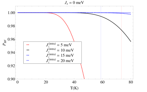
Figure S1: The behaviour of probability $P_{BF}(T)$ with respect to changes in the energy of ionic defect penalty when the orbital interaction energy vanishes. Vertical solid lines coloured blue and red respectively pinpoint the experimentally determined phase transition temperatures $58.9$ K and $73.4$ K 2015_HexPhaseTransition .

Table 2: Dependence of $P_{BF}(T)$ and $S(T)$ to $J_{x}$ when $J_{z}^{(\text{intra})}=+10$ meV.

$J_{x}(\text{meV})$	$S(20\,\text{K})$	$P_{BF}(20\,\text{K})$	$P_{BF}(58.9\,\text{K})$	$P_{BF}(73.4\,\text{K})$
$-1.00$	$1.00$	$0.98$	$0.98$	$0.96$
$-0.90$	$1.00$	$0.99$	$0.98$	$0.96$
$-0.80$	$1.00$	$0.99$	$0.98$	$0.96$
$-0.70$	$1.00$	$0.99$	$0.99$	$0.97$
$-0.60$	$1.00$	$0.99$	$0.99$	$0.97$
$-0.50$	$1.00$	$1.00$	$0.99$	$0.97$
$-0.40$	$1.00$	$1.00$	$0.99$	$0.97$
$-0.30$	$1.00$	$1.00$	$0.99$	$0.97$
$-0.20$	$1.00$	$1.00$	$0.99$	$0.97$
$-0.10$	$1.00$	$1.00$	$0.99$	$0.97$
$-0.00$	$1.00$	$1.00$	$0.99$	$0.97$

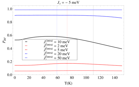
Figure S2: The behaviour of probability $P_{BF}(T)$ with respect to further changes in the energy of ionic defect penalty after the orbital interaction energy is reduced to a value lower than the fixed value used in the manuscript.

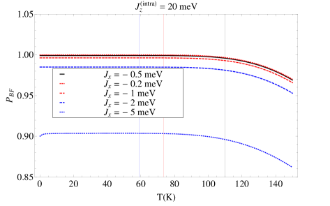
Figure S3: The behaviour of probability $P_{BF}(T)$ with respect to further changes in the orbital interaction energy after the energy of ionic defect penalty is raised to a value higher than the fixed value used in the manuscript.

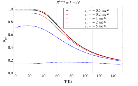
Figure S4: The behaviour of probability $P_{BF}(T)$ with respect to further changes in the orbital interaction energy after the energy of ionic defect penalty is reduced to a value lower than the fixed value used in the manuscript.