Two-photon exchange interaction from Dicke Hamiltonian under parametric modulation

Abstract

We consider the nonstationary circuit QED architecture in which a single-mode cavity interacts with $N>1$ identical qubits, and some system parameters undergo a weak external perturbation. It is shown that in the dispersive regime one can engineer the two-photon exchange interaction by adjusting the frequency of harmonic modulation to (approximately) $2|\Delta_{-}|$, where $\Delta_{-}$ is the average atom–field detuning. Closed analytic description is derived for the weak atom–field coupling regime, and numeric simulations indicate that the phenomenon can be observed in the present setups.

I Introduction

The area of circuit Quantum Electrodynamics (circuit QED) has grown to embrace a plethora of architectures with different kinds of multi-level atoms and sophisticated assemblies of interconnected 3D and 1D resonators and waveguides paik ; you ; science ; rev1 ; APL ; rev2 ; nori2017 . Diverse designs incorporating up to tens of Josephson Junctions give rise to superconducting artificial atoms with distinct properties regarding the dissipation mechanisms and the structure of energy levels, however, all they share the capability of coherently coupling to the Electromagnetic (EM) field nor ; smith ; reagor ; wilson ; ofec ; wallr . Moreover, a single cavity mode can interact with several locally addressable artificial atoms 3at0 ; 3at1 ; 3at2 ; ann ; cle ; saito ; gam1 ; song or an ensemble of trapped ultracold atoms uatoms1 ; uatoms2 .

Many types of superconducting artificial atoms allow for real-time manipulation of the energy levels or the atom–field coupling strength majer ; ge ; ger ; ger1 ; v1 ; v2 ; v3 . Combined with the ability of in situ tuning the resonator’s frequency by external magnetic flux nori-n ; meta , such nonstationary circuit QED architectures give rise to a novel regime of light–matter interaction in which all the parameters in the Hamiltonian are controllable functions of time jpcs ; JPA . Using resonant perturbations one can induce creation and annihilation of photons or atomic excitations liberato9 ; roberto ; diego ; etc1 ; juan ; hoeb , generate entanglement entangles ; etc3 ; enta2 , induce new forms of light–matter interaction igor ; porras ; palermo ; tom , perform quantum simulations relativistic ; sim and study other novel effects etc2 ; processing ; ert ; ert2 . Some of the early proposals jpcs ; bla have recently been verified experimentally, such as the one-photon exchange between the qubit and the field in the dispersive regime (reliant on the ‘rotating’ terms in the interaction Hamiltonian) blais-exp ; simmonds and generation of two quanta from vacuum due to the ‘counter-rotating terms’ (CRT) schuster .

In this paper we describe another effect based on the rotating terms – the two-photon exchange interaction – that can be implemented in nonstationary circuit QED by modulating any system parameter with frequency $\eta\approx 2|\Delta_{-}|$, where $\Delta_{-}$ is the average atom–field detuning. We illustrate the phenomenon for the case of $N>1$ off-resonant qubits described by the Dicke dicke ; HP or Tavis-Cummings TC1 ; TC2 Hamiltonians, however, our approach can be straightforwardly generalized to an arbitrary multilevel atom in the ladder configuration JPA . Assuming the weak atom–field coupling regime, we derive a closed analytic description of the unitary dynamics (see Sec. II) and find a good agreement with numeric data even for moderate coupling strengths (Sec. III). We also show that our proposal can be implemented in the current circuit QED setups with weak dissipation and slightly different atoms (Sec. III.1), and discuss manners to enhance the two-photon transition rate.

II Analytic results

Our system consists of a single mode of EM field interacting with $N$ qubits, as described by the quantum Dicke model dicke ; HP

$$\hat{H}/\hbar=\omega\hat{n}+\sum_{l=1}^{N}\left[\frac{\Omega}{2}\hat{\sigma}_{z}^{(l)}+g(\hat{a}+\hat{a}^{\dagger})(\hat{\sigma}_{+}^{(l)}+\hat{\sigma}_{-}^{(l)})\right]\leavevmode\nobreak\ ,$$ (1)

where the index $l$ labels the identical noninteracting atoms. We assume that the cavity frequency $\omega$, the atomic transition frequency $\Omega$ and the atom–cavity coupling strength$\leavevmode\nobreak\ g$ are externally prescribed functions of time ($g$ is considered real). $\hat{a}$ and $\hat{a}^{\dagger}$ are the annihilation and creation operators and $\hat{n}=\hat{a}^{\dagger}\hat{a}$ is the photon number operator. The qubit operators are $\hat{\sigma}_{-}^{(l)}=|g^{(l)}\rangle\langle e^{(l)}|$, $\hat{\sigma}_{+}^{(l)}=|e^{(l)}\rangle\langle g^{(l)}|$ and $\hat{\sigma}_{z}^{(l)}=|e^{(l)}\rangle\langle e^{(l)}|-|g^{(l)}\rangle\langle g^{(l)}|$, where $|g^{(l)}\rangle$ and $|e^{(l)}\rangle$ denote the ground and excited states of the $l$-th qubit, respectively. In the absence of CRT $\sum_{l=1}^{N}(\hat{a}\hat{\sigma}_{-}^{(l)}+\hat{a}^{\dagger}\hat{\sigma}_{+}^{(l)})$ the Hamiltonian (1) is known as Tavis-Cummings Hamiltonian TC1 ; TC2 . We stress that although our approach takes into account the CRT, the phenomenon described in this paper does not require their presence.

We consider the general case of simultaneous external modulation of all the system parameters as $X=X_{0}+\varepsilon_{X}\sin(\eta t+\phi_{X})$, where $X$ stands for $\omega$, $\Omega$ or $g$ (for the particular case of a single-parameter modulation, only one $\varepsilon_{X}$ is nonzero). $X_{0}$ is the bare value, $\varepsilon_{X}\geq 0$ is the respective modulation depth, $\eta\sim 2|\omega_{0}-\Omega_{0}|$ is the modulation frequency and $\phi_{X}$ is the initial phase. Moreover, we restrict our analysis to the perturbative regime when $\varepsilon_{g}\ll g_{0}$ and $\varepsilon_{\omega},\varepsilon_{\Omega}\ll|\omega_{0}-\Omega_{0}|$.

To obtain closed analytical description we employ the normalized Dicke states with $k$ atomic excitations

$$|\mathbf{k}\rangle=\sqrt{\frac{k!(N-k)!}{N!}}\sum_{p}|e^{\left(1\right)}\rangle|e^{\left(2\right)}\rangle\cdots|e^{\left(k\right)}\rangle|g^{\left(k+1\right)}\rangle\cdots|g^{N}\rangle,$$ (2)

where the sum runs over all the allowed permutations of excited and non-excited qubits and $k=0,1,\ldots,N$. In the Dicke basis the Hamiltonian (1) reads

$$\hat{H}/\hbar=\omega\hat{n}+\sum_{k=0}^{N}[\Omega k\hat{\sigma}_{k,k}+gf_{k}(\hat{a}+\hat{a}^{\dagger})(\hat{\sigma}_{k+1,k}+\hat{\sigma}_{k,k+1})],$$ (3)

where $\hat{\sigma}_{k,j}\equiv|\mathbf{k}\rangle\langle\mathbf{j}|$ and $f_{k}\equiv\sqrt{(k+1)(N-k)}$.

We work in the dispersive regime, $g_{0}f_{k}\sqrt{n}\ll|\Delta_{-}|$ for all relevant values of $n$, where $\Delta_{-}=\omega_{0}-\Omega_{0}$ is the bare atom–field detuning and $n$ is the total number of excitations. Following the approach described in JPA ; juan , we expand the system state as

$$|\psi(t)\rangle=\sum_{m=0}^{\infty}\sum_{\mathcal{S}}e^{i\Phi_{m,\mathcal{S}}(t)}e^{-it\tilde{\lambda}_{m,\mathcal{S}}}b_{m,\mathcal{S}}(t)|\varphi_{m,\mathcal{S}}\rangle\leavevmode\nobreak\ .$$ (4)

$\Phi_{m,\mathcal{S}}(t)$ is a real oscillatory function

$$\Phi_{m,\mathcal{S}}(t)=\sum_{k=0}^{N}\sum_{L=\omega,g,\Omega}\frac{\Upsilon_{m,\mathcal{S},\mathcal{S}}^{L,k}}{\eta}\left[\cos(\eta t+\phi_{L})-\cos\phi_{L}\right]\,,\leavevmode\nobreak\$$ (5)

where we defined the constant coefficients

$$\Upsilon_{m,\mathcal{T},\mathcal{S}}^{\omega,k}\equiv\delta_{k,0}\varepsilon_{\omega}\langle\varphi_{m,\mathcal{T}}|\hat{n}|\varphi_{m,\mathcal{S}}\rangle$$ (6)

$$\Upsilon_{m,\mathcal{T},\mathcal{S}}^{g,k}\equiv\varepsilon_{g}f_{k}\langle\varphi_{m,\mathcal{T}}|(\hat{a}\hat{\sigma}_{k+1,k}+\hat{a}^{\dagger}\hat{\sigma}_{k,k+1})|\varphi_{m,\mathcal{S}}\rangle$$ (7)

$$\Upsilon_{m,\mathcal{T},\mathcal{S}}^{\Omega,k}\equiv\varepsilon_{\Omega}k\langle\varphi_{m,\mathcal{T}}|\hat{\sigma}_{k,k}|\varphi_{m,\mathcal{S}}\rangle$$ (8)

and assumed that $|\Upsilon_{n,\mathcal{T},\mathcal{S}}^{L,k}/\Delta_{-}|\ll 1$ for $L=\omega,g,\Omega$ and all relevant values of $k,n$, $\mathcal{T}$ and $\mathcal{S}$.

$\tilde{\lambda}_{m,\mathcal{S}}\equiv\lambda_{m,\mathcal{S}}+\nu_{m,\mathcal{S}}$ is the effective eigenfrequency, where $\lambda_{m,\mathcal{S}}$ and $|\varphi_{m,\mathcal{S}}\rangle$ are the $m$-excitations eigenfrequencies and eigenstates (dressed states) of the bare Hamiltonian

$$\hat{H}_{0}/\hbar=\omega_{0}\hat{n}+\sum_{k=0}^{N}[\Omega_{0}k\hat{\sigma}_{k,k}+g_{0}f_{k}(\hat{a}\hat{\sigma}_{k+1,k}+\hat{a}^{\dagger}\hat{\sigma}_{k,k+1})]\,.$$ (9)

The index $\mathcal{S}$ labels the different eigenvalues and eigenstates within the subspace of a given value of $m$. $\nu_{m,\mathcal{S}}\sim\mathcal{O}(g_{0}^{2}/\omega_{0})$ is the frequency shift juan due to the counter-rotating terms in Eq. (3):

$$\nu_{m,\mathcal{T}} = g_{0}^{2}\sum_{\mathcal{S}}\left[\frac{\left(\sum_{k=0}^{N}f_{k}\Lambda_{k,m,\mathcal{S},\mathcal{T}}\right)^{2}}{\lambda_{m,\mathcal{T}}-\lambda_{m-2,\mathcal{S}}}\right.$$ (10)

$$\left.-\frac{\left(\sum_{k=0}^{N}f_{k}\Lambda_{k,m+2,\mathcal{T},\mathcal{S}}\right)^{2}}{\lambda_{m+2,\mathcal{S}}-\lambda_{m,\mathcal{T}}}\right]$$

$$\Lambda_{k,m+2,\mathcal{T},\mathcal{S}}\equiv\langle\varphi_{m,\mathcal{T}}|\hat{a}\hat{\sigma}_{k,k+1}|\varphi_{m+2,\mathcal{S}}\rangle\,,$$ (11)

where we assumed $g_{0}f_{k}\Lambda_{k,m+2,\mathcal{S},\mathcal{T}}\lesssim\omega_{0}-\left|\Delta_{-}\right|$. Lastly, $b_{m,\mathcal{S}}(t)$ is the slowly-varying probability amplitude for the dressed state $|\varphi_{m,\mathcal{S}}\rangle$.

Substituting (4) into the Schrödinger equation and neglecting the rapidly oscillating terms JPA , we obtain to the first order in $\varepsilon_{\omega}$, $\varepsilon_{g}$ and $\varepsilon_{\Omega}$

$$\dot{b}_{n,\mathcal{T}}=\sum_{\mathcal{S}\neq\mathcal{T}}\Xi_{n,\mathcal{T},\mathcal{S}}e^{its_{n,\mathcal{T},\mathcal{S}}(|\tilde{\lambda}_{n,\mathcal{T}}-\tilde{\lambda}_{n,\mathcal{S}}|-\eta)}b_{n,\mathcal{S}}\leavevmode\nobreak\ ,$$ (12)

where $s_{n,\mathcal{T},\mathcal{S}}\equiv\mathrm{sign}(\tilde{\lambda}_{n,\mathcal{T}}-\tilde{\lambda}_{n,\mathcal{S}})$ and

$$\Xi_{n,\mathcal{T},\mathcal{S}}\equiv\frac{s_{n,\mathcal{T},\mathcal{S}}}{2}\sum_{k=0}^{N}\sum_{L=g,\Omega,\omega}\Upsilon_{n,\mathcal{T},\mathcal{S}}^{L,k}e^{-is_{n,\mathcal{T},\mathcal{S}}\phi_{L}}\leavevmode\nobreak\ ,$$ (13)

$\Xi_{n,\mathcal{T},\mathcal{S}}^{\ast}=-\Xi_{n,\mathcal{S},\mathcal{T}}$. To obtain Eq. (12) we neglected frequency shifts smaller than $\nu_{n,\mathcal{T}}$, as well as the corrections of the order of $(\Upsilon_{n,\mathcal{T},\mathcal{S}}^{L,k})^{2}/\Delta_{-}\propto\varepsilon_{L}^{2}/\Delta_{-}$ for $L=\omega,g,\Omega$.

Under the resonant modulation frequency, $\eta_{res}=|\tilde{\lambda}_{n,\mathcal{T}}-\tilde{\lambda}_{n,\mathcal{S}}|$, we get

$$b_{n,\mathcal{T}}=b_{n,\mathcal{T}}\left(0\right)\cos|\Xi_{n,\mathcal{T},\mathcal{S}}|t+\frac{\Xi_{n,\mathcal{T},\mathcal{S}}}{|\Xi_{n,\mathcal{T},\mathcal{S}}|}b_{n,\mathcal{S}}\left(0\right)\sin|\Xi_{n,\mathcal{T},\mathcal{S}}|t\,,$$ (14)

corresponding to the modulation-induced transition $|\varphi_{n,\mathcal{T}}\rangle\leftrightarrow|\varphi_{n,\mathcal{S}}\rangle$. We emphasize that, under the considered approximations, Eqs. (12) – (13) also describe the effective dynamics in the absence of CRT in the Hamiltonian (3), though in this case the frequency shift $\nu_{m,\mathcal{T}}=0$ so that $\tilde{\lambda}_{n,\mathcal{T}}=\lambda_{n,\mathcal{T}}$ .

In the dispersive regime the spectrum of $\hat{H}_{0}$ can be obtained from the standard perturbation theory. To the second order in $g_{0}/\Delta_{-}$ one finds

$$\lambda_{n,k}=n\omega_{0}-k\Delta_{-}+\delta_{-}\left[(N-k)(n-2k)-k(n-k+1)\right]$$

$$|\varphi_{n,k}\rangle = \mathcal{N}_{n,k}\left[|\varphi_{n,k}^{\left(0\right)}\rangle+\frac{g_{0}f_{k}\sqrt{K}}{\Delta_{-}}|\varphi_{n,k+1}^{\left(0\right)}\rangle\right.$$

$$-\frac{g_{0}f_{k-1}\sqrt{K+1}}{\Delta_{-}}|\varphi_{n,k-1}^{\left(0\right)}\rangle$$

$$+\frac{g_{0}^{2}f_{k}f_{k+1}\sqrt{K\left(K-1\right)}}{2\Delta_{-}^{2}}|\varphi_{n,k+2}^{\left(0\right)}\rangle$$

$$\left.+\frac{g_{0}^{2}f_{k-1}f_{k-2}\sqrt{\left(K+1\right)\left(K+2\right)}}{2\Delta_{-}^{2}}|\varphi_{n,k-2}^{\left(0\right)}\rangle\right],$$

where $k=0,1,2,...,\min\left(n,N\right)$, $K=n-k$, $\delta_{-}=g_{0}^{2}/\Delta_{-}$, $|\varphi_{n,k}^{\left(0\right)}\rangle=|\mathbf{k},n-k\rangle\equiv|\mathbf{k}\rangle_{atom}\otimes|n-k\rangle_{field}$ and $\mathcal{N}_{n,k}$ is the normalization constant ($|n\rangle_{field}$ is the cavity Fock state). Actually, to evaluate the two-photon transition rate one needs the eigenstates to the fourth order in $g_{0}/\Delta_{-}$, which are omitted here for brevity.

The two-photon exchange interaction chen ; alexanian ; chen2 corresponds to the transition $|\varphi_{n,k}\rangle\leftrightarrow|\varphi_{n,k+2}\rangle$, which represents (approximately) $|\mathbf{k},n-k\mathbf{\rangle}\leftrightarrow|\mathbf{k+2},n-k-2\rangle$. To the lowest order in $g_{0}/\Delta_{-}$ we obtain

$$\Xi_{n,k,k+2} = \mathcal{D}g_{0}\left(\frac{g_{0}}{\Delta_{-}}\right)^{3}\sqrt{(N-k)(N-k-1)}$$

$$\times\sqrt{(k+1)(k+2)K(K-1)}$$

$$\times\left(\frac{\varepsilon_{\omega}e^{-i\mathcal{D}\phi_{\omega}}}{\Delta_{-}}-\frac{\varepsilon_{\Omega}e^{-i\mathcal{D}\phi_{\Omega}}}{\Delta_{-}}-\frac{\varepsilon_{g}e^{-i\mathcal{D}\phi_{g}}}{g_{0}}\right),$$

where $\mathcal{D}=\mathrm{sign}(\Delta_{-})$. The corresponding resonant modulation frequency reads

$$\eta_{r}\approx 2\left|\Delta_{-}+\delta_{-}(2N+2n-6k-5)\right|\,.$$ (17)

Notice that for a given value of $k$ the other states $\{|\mathbf{k},n^{\prime}-k\mathbf{\rangle,}|\mathbf{k+2},n^{\prime}-k-2\rangle\}$ ($n^{\prime}\neq n$) are not affected by such modulation due to the condition $|\delta_{-}|\gg|\Xi_{n,k,k+2}|$, as can be seen from Eq. (12). So in the most common situation when the atoms are initially in the ground states (the Dicke state $|\mathbf{0}\rangle$) only the pair of states selected by the modulation frequency becomes coupled. On the other hand, if the atoms are prepared in a superposition of Dicke states, several states can become coupled by a single modulation frequency. For example, from Eq. (17) we see that to the second order in $g_{0}/\Delta_{-}$ the same frequency $\eta_{r}$ couples the pair of states $|\mathbf{0},4\mathbf{\rangle\leftrightarrow}|\mathbf{2},2\mathbf{\rangle}$ and $|\mathbf{1},6\mathbf{\rangle\leftrightarrow}|\mathbf{3},4\mathbf{\rangle}$; we verified that for certain values of parameters this fact persists to the fourth order in $g_{0}/\Delta_{-}$ as well.

III Numeric results

Figure 1: (Color online) Comparison of the approximate analytic and exact numeric results (with and without CRT) for $N=2$. The initial state is $|\mathbf{0}\rangle\otimes|5\rangle$. $n_{ph}$ and $n_{at}$ stand for the average numbers of photons and atomic excitations, respectively.

Figure 2: (Color online) Exact numeric dynamics of the average excitation numbers under the sole $g$-modulation (black) and the simultaneous modulation of $g$ and $\Omega$ (red). The initial state is $|\mathbf{0}\rangle\otimes|\alpha\rangle$, $\alpha=5.5$ and $N=6$.

To check our analytic predictions we solved numerically the Schrödinger equation for the original Hamiltonian (1). In Fig. 1 we compare the exact numeric results, with and without CRT, to the approximate formulas (13) – (14). We plot the average number of photons $n_{ph}=\langle\psi|\hat{n}|\psi\rangle$ and the average number of atomic excitations $n_{at}=\langle\psi|\sum_{k=1}^{N}k\sigma_{k,k}|\psi\rangle$ for the initial state $|\mathbf{0}\rangle\otimes|5\rangle$ and parameters $N=2$, $g_{0}\sqrt{N}/\omega_{0}=8\times 10^{-2}$, $\Delta_{-}=-9g_{0}\sqrt{N}$, $\varepsilon_{g}/g_{0}=10^{-1}$, $\phi_{g}=0$, $\varepsilon_{\Omega}=\varepsilon_{\omega}=0$. As expected, the resonant modulation frequencies vary depending on whether the CRT are taken into account or not: $\eta_{r}=2|\Delta_{-}|\times 1.0678$ with CRT and $\eta_{r}=2|\Delta_{-}|\times 1.0540$ without CRT. The analytic and numeric results agree qualitatively, though there is a roughly $20\%$ difference in the analytic and actual transition rates $|\Xi_{5,0,2}|$. Such discrepancy is not surprising, since for the above parameters the required inequalities $\sqrt{2n}g_{0}/\Delta_{-}\ll 1$ and $|\Delta_{-}|\ll\omega_{0}$ are only barely satisfied foot1 . The apparent broad width of the curves is explained by fast low-amplitude oscillations due to the off-resonant photon exchange inherent to the dispersive regime, as inferred from the wavefunction (4) and the expression for the dressed states (II).

In Fig. 2 we consider a more realistic initial state $|\mathbf{0}\rangle\otimes|\alpha\rangle$, where $|\alpha\rangle=e^{-|\alpha|^{2}/2}\sum_{n=0}^{\infty}\alpha^{n}/\sqrt{n!}$ stands for the cavity coherent state with $\alpha=\sqrt{5.5}$ [so that the initial probability of 5 photons is $P_{ph}(5)\approx 0.17$]. For the sake of compactness we only present the exact numeric results in the presence of CRT. We set $N=6$ and consider the $g$-modulation (with parameters $g_{0}\sqrt{N}/\omega_{0}=8\times 10^{-2}$, $\Delta_{-}=-9g_{0}\sqrt{N}$, $\varepsilon_{g}/g_{0}=10^{-1}$, $\phi_{g}=0$ and $\eta_{r}=2|\Delta_{-}|\times 1.0389$), as well as the simultaneous modulation of $g$ and $\Omega$ with the additional parameters $\varepsilon_{\Omega}/|\Delta_{-}|=10^{-1}$ and $\phi_{\Omega}=\pi$ (in this case $\eta_{r}=2|\Delta_{-}|\times 1.0388$). These modulation frequencies were adjusted to promote the transition $|\mathbf{0},5\rangle\leftrightarrow|\mathbf{2},3\rangle$, and we defined $q\equiv|\Xi_{5,0,2}(\varepsilon_{\Omega}=\varepsilon_{\omega}=0)|$ (i. e., $q$ is the transition rate under the pure $g$-modulation). We observe that excitations are transferred between the cavity and far-detuned atoms, and under the simultaneous $g$- and $\Omega$-modulations the oscillations are roughly twice faster than under the sole $g$-modulation, in agreement with Eq. (II).

To attest that the periodic behavior of $n_{ph}$ and $n_{at}$ indeed corresponds to a two-photon exchange, in Fig. 3 we plot the probability $P_{ph}(k)$ of $k$ photons and the probability $P_{at}(m)$ of $m$ atomic excitations under the simultaneous $g$- and $\Omega$-modulations (discussed in Fig. 2). We observe that the main transition occurs between the states $|\mathbf{0},5\rangle\$and $|\mathbf{2},3\rangle$, although there are unwanted couplings between other states owing to the off-resonant one-photon exchange. As an example, we illustrate small oscillations between the states $|\mathbf{2},3\rangle\leftrightarrow|\mathbf{3},2\rangle$, inferred from the periodic oscillation of probabilities $P_{ph}(2)$ and $P_{at}(3)$ at the same rate as the probabilities $P_{ph}(3)$ and $P_{at}(2)$.

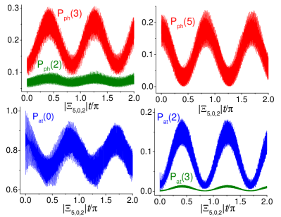
Figure 3: (Color online) Exact numeric dynamics of probabilities $P_{ph}(k)$ and $P_{at}(m)$ for $N=6$ and the simultaneous modulation of $g$ and $\Omega$. The initial state is $|\mathbf{0}\rangle\otimes|\alpha\rangle$, $\alpha=\sqrt{5.5}$, and the modulation induces the transition $|\mathbf{0},5\rangle\rightarrow|\mathbf{2},3\rangle$.

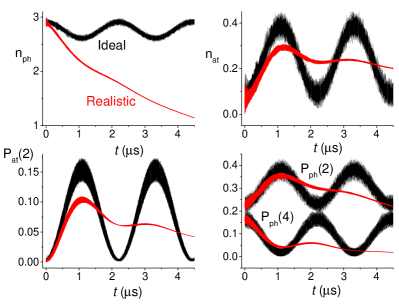
Figure 4: (Color online) Comparison of the dynamics under realistic and ideal conditions in two-qubit circuit QED architecture. Here we consider the $g$-modulations of both qubits, $\omega_{0}/2\pi=10\,$GHz and the initial state $|g^{(1)},g^{(2)}\rangle\otimes|\alpha\rangle$, $\alpha=\sqrt{3}$. The modulation drives the transition $|\mathbf{0},4\rangle\leftrightarrow|\mathbf{2},2\rangle$.

III.1 Simulation under realistic conditions

The above numeric results apply to an ideal situation, namely, strictly identical atoms and dissipation-free environment. To asses the experimental feasibility of our proposal in circuit QED, we consider a realistic scenario of two slightly different artificial atoms coupled to a single-mode waveguide resonator under weak Markovian dissipation. The dynamics is now governed by the master equation

$$d\hat{\rho}/dt=\frac{1}{i\hbar}[\tilde{H},\hat{\rho}]+\mathcal{\hat{L}}\hat{\rho}$$ (18)

$$\tilde{H}/\hbar=\omega\hat{n}+\sum_{l=1}^{2}\left[\frac{\Omega^{(l)}}{2}\hat{\sigma}_{z}^{(l)}+g^{(l)}(\hat{a}+\hat{a}^{\dagger})(\hat{\sigma}_{+}^{(l)}+\hat{\sigma}_{-}^{(l)})\right]\leavevmode\nobreak\ ,$$

where $\hat{\rho}$ is the total density operator and $\mathcal{\hat{L}}$ is the Liouvillian. To get a rough estimative we solved numerically the ‘standard’ phenomenological master equation bla for zero-temperature reservoirs foot2

$$\mathcal{\hat{L}}\hat{\rho}=\kappa\mathcal{D}[\hat{a}]\hat{\rho}+\sum_{l=1}^{2}\left(\gamma^{(l)}\mathcal{D}[\hat{\sigma}_{-}^{(l)}]+\frac{\gamma_{\phi}^{(l)}}{2}\mathcal{D}[\hat{\sigma}_{z}^{(l)}]\right)\hat{\rho}\,,$$ (19)

where $\mathcal{D}[\hat{O}]\hat{\rho}\equiv(2\hat{O}\hat{\rho}\hat{O}^{\dagger}-\hat{O}^{\dagger}\hat{O}\hat{\rho}-\hat{\rho}\hat{O}^{\dagger}\hat{O})/2$ is the Lindbladian superoperator. The constant parameters $\kappa$, $\gamma^{(l)}$ and $\gamma_{\phi}^{(l)}$ denote the cavity damping and the $l$-th qubit’s relaxation and pure dephasing rates, respectively.

In Fig. 4 we compare the dynamics for the ideal and realistic scenarios under the $g$-modulations and the initial cavity coherent state $|g^{(1)},g^{(2)}\rangle\otimes|\alpha\rangle$, where $\alpha=\sqrt{3}$. For the realistic case we set: $g^{(l)}=g_{0}^{(l)}+\varepsilon_{g}^{(l)}\sin(\eta t)$, $g_{0}^{(1)}/\omega_{0}=5.66\times 10^{-2}$, $g_{0}^{(2)}=1.01g_{0}^{(1)}$, $\varepsilon_{g}^{(l)}/g_{0}^{(l)}=0.1$, $\Delta_{-}^{(1)}\equiv\omega_{0}-\Omega^{(1)}=-0.72\omega_{0}$, $\Delta_{-}^{(2)}=1.02\Delta_{-}^{(1)}$, $\kappa/g_{0}^{(1)}=\gamma^{(l)}/g_{0}^{(l)}=5\times 10^{-5}$, $\gamma_{\phi}^{(l)}=\gamma^{(l)}$ and $\eta_{r}=2|\Delta_{-}^{(1)}|\times 1.0632$. For the ideal case $g_{0}/\omega_{0}=5.66\times 10^{-2}$, $\varepsilon_{g}/g_{0}=0.1$, $\Delta_{-}=-0.72\omega_{0}$ and $\eta_{r}=2|\Delta_{-}|\times 1.0531$ (the modulation frequencies were chosen to induce the transition $|\mathbf{0},4\rangle\leftrightarrow|\mathbf{2},2\rangle$). Such parameters are compatible with the current circuit QED architectures, where typically $\omega_{0}/2\pi=10\,$GHz paik ; ger ; 3at0 ; 3at1 ; 3at2 ; saito ; reagor ; ofec ; schuster . We see that for initial times, $t\lesssim 1\,\mu$s, the two-photon exchange can be proved via measurements of the average number of atomic excitations $n_{at}$ or the probabilities $P_{at}(2)$, $P_{ph}(2)$ and $P_{ph}(4)$, whereas the measurement of the average photon number is of little help due to overwhelming effects of dissipation.

IV Conclusions

We showed analytically and numerically that effective two-photon exchange interaction between a single cavity mode and $N>1$ off-resonant qubits can be achieved by externally modulating any system parameter at frequency $\eta\approx 2|\Delta_{-}|$, where $\Delta_{-}$ is the average atom–field detuning. This effect originates from the ‘rotating’ terms in the Dicke (or Tavis-Cummings) Hamiltonian, but the associated transition rate is quite small due to the multiplicative factor $(g_{0}/\Delta_{-})^{3}$. Closed analytical description was derived under the assumption of weak atom–field coupling, and a good agreement with exact numeric results was observed even for moderate coupling strengths. For a simultaneous modulation of different parameters the transition rate can be increased by properly adjusting the initial phases. Regarding the experimental feasibility, we demonstrated that for $N=2$ our proposal can be implemented in the current circuit QED architectures on the timescales $\sim 1\,\mu$s, which could be further reduced through an increase in the modulation amplitudes, atom–field coupling strength or the number of qubits.

- (1) H. Paik, D. I. Schuster, L. S. Bishop, G. Kirchmair, G. Catelani, A. P. Sears, B. R. Johnson, M. J. Reagor, L. Frunzio, L. I. Glazman, S. M. Girvin, M. H. Devoret, and R. J. Schoelkopf, Observation of High Coherence in Josephson Junction Qubits Measured in a Three-Dimensional Circuit QED Architecture, Phys. Rev. Lett. 107, 240501 (2011).
- (2) J. Q. You and F. Nori, Atomic physics and quantum optics using superconducting circuits, Nature 474, 589 (2011).
- (3) M. H. Devoret and R. J. Schoelkopf, Superconducting Circuits for Quantum Information: An Outlook, Science 339, 1169 (2013).
- (4) S. Schmidt and J. Koch, Circuit QED lattices: Towards quantum simulation with superconducting circuits, Ann. Phys. (Berlin) 525, 395 (2013).
- (5) C. Axline, M. Reagor, R. Heeres, P. Reinhold, C. Wang, K. Shain, W. Pfaff, Y. Chu, L. Frunzio, and R. J. Schoelkopf, An architecture for integrating planar and 3D cQED devices, Appl. Phys. Lett. 109 042601 (2016).
- (6) G. Wendin, Quantum information processing with superconducting circuits: a review, Rep. Prog. Phys. 80, 106001 (2017).
- (7) X. Gu, A. F. Kockum, A. Miranowicz,Yu-xi Liu, and F. Nori, Microwave photonics with superconducting quantum circuits, Phys. Rep. 718-719, 1 (2017).
- (8) Yu-xi Liu, J. Q. You, L. F. Wei, C. P. Sun, and F. Nori, Optical Selection Rules and Phase-Dependent Adiabatic State Control in a Superconducting Quantum Circuit, Phys. Rev. Lett. 95, 087001 (2005).
- (9) W. C. Smith, A. Kou, U. Vool, I. M. Pop, L. Frunzio, R. J. Schoelkopf, and M. H. Devoret, Quantization of inductively shunted superconducting circuits, Phys. Rev. B 94, 144507 (2016).
- (10) M. Reagor, W. Pfaff, C. Axline, R. W. Heeres, N. Ofek, K. Sliwa, E. Holland, C. Wang, J. Blumoff, K. Chou, M. J. Hatridge, L. Frunzio, M. H. Devoret, L. Jiang, and R. J. Schoelkopf, Quantum memory with millisecond coherence in circuit QED, Phys. Rev. B 94, 014506 (2016).
- (11) P. Forn-Díaz, J. J. García-Ripoll, B. Peropadre, J. -L. Orgiazzi, M. A. Yurtalan, R. Belyansky, C. M. Wilson, and A. and Lupascu, Ultrastrong coupling of a single artificial atom to an electromagnetic continuum in the nonperturbative regime, Nat. Phys. 13, 39 (2017).
- (12) N. Ofek, A. Petrenko, R. Heeres, P. Reinhold, Z. Leghtas, B. Vlastakis, Y. Liu, L. Frunzio, S. M. Girvin, L. Jiang, M. Mirrahimi, M. H. Devoret, and R. J. Schoelkopf, Extending the lifetime of a quantum bit with error correction in superconducting circuits, Nature 536 441 (2016).
- (13) S. Gasparinetti, M. Pechal, J.-C. Besse, M. Mondal, C. Eichler, and A. Wallraff, Correlations and Entanglement of Microwave Photons Emitted in a Cascade Decay, Phys. Rev. Lett. 119, 140504 (2017).
- (14) J. M. Fink, R. Bianchetti, M. Baur, M. Göppl, L. Steffen, S. Filipp, P. J. Leek, A. Blais, and A. Wallraff, Dressed Collective Qubit States and the Tavis-Cummings Model in Circuit QED, Phys. Rev. Lett. 103, 083601 (2009).
- (15) M. Neeley, R. C. Bialczak, M. Lenander, E. Lucero, M. Mariantoni, A. D. O’Connell, D. Sank, H. Wang, M. Weides, J. Wenner, Y. Yin, T. Yamamoto, A. N. Cleland, and J. M. Martinis, Generation of three-qubit entangled states using superconducting phase qubits, Nature 467, 570 (2010).
- (16) L. DiCarlo, M. D. Reed, L. Sun, B. R. Johnson, J. M. Chow, J. M. Gambetta, L. Frunzio, S. M. Girvin, M. H. Devoret, and R. J. Schoelkopf, Preparation and measurement of three-qubit entanglement in a superconducting circuit, Nature 467, 574 (2010).
- (17) M. W. Johnson, M. H. S. Amin, S. Gildert, T. Lanting, F. Hamze, N. Dickson, R. Harris, A. J. Berkley, J. Johansson, P. Bunyk, E. M. Chapple, C. Enderud, J. P. Hilton, K. Karimi, E. Ladizinsky, N. Ladizinsky, T. Oh, I. Perminov, C. Rich, M. C. Thom, E. Tolkacheva, C. J. S. Truncik, S. Uchaikin, J. Wang, B. Wilson, and G. Rose, Quantum annealing with manufactured spins, Nature 473, 194 (2011).
- (18) R. Barends, J. Kelly, A. Megrant, A. Veitia, D. Sank, E. Jeffrey, T. C. White, J. Mutus, A. G. Fowler, B. Campbell, Y. Chen, Z. Chen, B. Chiaro, A. Dunsworth, C. Neill, P. O’Malley, P. Roushan, A. Vainsencher, J. Wenner, A. N. Korotkov, A. N. Cleland, and J. M. Martinis, Superconducting quantum circuits at the surface code threshold for fault tolerance, Nature 508, 500 (2014).
- (19) K. Kakuyanagi, Y. Matsuzaki, C. Déprez, H. Toida, K. Semba, H. Yamaguchi, W. J. Munro, and S. Saito, Observation of Collective Coupling between an Engineered Ensemble of Macroscopic Artificial Atoms and a Superconducting Resonator, Phys. Rev. Lett. 117, 210503 (2016).
- (20) M. Takita, A. W. Cross, A. D. Córcoles, J. M. Chow, and J. M. Gambetta, Experimental Demonstration of Fault-Tolerant State Preparation with Superconducting Qubits, Phys. Rev. Lett. 119, 180501 (2017).
- (21) C. Song, K. Xu, W. Liu, C. Yang, S. Zheng, H. Deng, Q. Xie, K. Huang, Q. Guo, L. Zhang, P. Zhang, D. Xu, D. Zheng, X. Zhu, H. Wang, Y.-A. Chen, C.-Y. Lu, S. Han, and J.-W. Pan, 10-Qubit Entanglement and Parallel Logic Operations with a Superconducting Circuit, Phys. Rev. Lett. 119, 180511 (2017).
- (22) J. Verdú, H. Zoubi, Ch. Koller, J. Majer, H. Ritsch, and J. Schmiedmayer, Strong Magnetic Coupling of an Ultracold Gas to a Superconducting Waveguide Cavity, Phys. Rev. Lett. 103, 043603 (2009).
- (23) H. Hattermann, D. Bothner, L. Y. Ley, B. Ferdinand, D. Wiedmaier, L. Sárkány, R. Kleiner, D. Koelle, and J. Fortágh, Coupling ultracold atoms to a superconducting coplanar waveguide resonator, Nat. Commun. 8, 2254 (2017).
- (24) J. Majer, J. M. Chow, J. M. Gambetta, J. Koch, B. R. Johnson, J. A. Schreier, L. Frunzio, D. I. Schuster, A. A. Houck, A. Wallraff, A. Blais, M. H. Devoret, S. M. Girvin, and R. J. Schoelkopf, Coupling superconducting qubits via a cavity bus, Nature 449, 443 (2007).
- (25) M. Hofheinz, H. Wang, M. Ansmann, R. C. Bialczak, E. Lucero, M. Neeley, A. D. O’Connell, D. Sank, J. Wenner, J. M. Martinis, and A. N. Cleland, Synthesizing arbitrary quantum states in a superconducting resonator, Nature 459, 546 (2009).
- (26) L. DiCarlo, J. M. Chow, J. M. Gambetta, L. S. Bishop, B. R. Johnson, D. I. Schuster, J. Majer, A. Blais, L. Frunzio, S. M. Girvin, and R. J. Schoelkopf, Demonstration of two-qubit algorithms with a superconducting quantum processor, Nature 460, 240 (2009).
- (27) J. Li, M. P. Silveri, K. S. Kumar, J. -M. Pirkkalainen, A. Vepsäläinen, W. C. Chien, J. Tuorila, M. A. Sillanpää, P. J. Hakonen, E. V. Thuneberg, and G. S. Paraoanu, Motional averaging in a superconducting qubit, Nat. Commun. 4, 1420 (2013).
- (28) S. J. Srinivasan, A. J. Hoffman, J. M. Gambetta, and A. A. Houck, Tunable Coupling in Circuit Quantum Electrodynamics Using a Superconducting Charge Qubit with a V-Shaped Energy Level Diagram, Phys. Rev. Lett. 106, 083601 (2011).
- (29) Y. Chen, C. Neill, P. Roushan, N. Leung, M. Fang, R. Barends, J. Kelly, B. Campbell, Z. Chen, B. Chiaro, A. Dunsworth, E. Jeffrey, A. Megrant, J. Y. Mutus, P. J. J. O’Malley, C. M. Quintana, D. Sank, A. Vainsencher, J. Wenner, T. C. White, M. R. Geller, A. N. Cleland, and J. M. Martinis, Qubit Architecture with High Coherence and Fast Tunable Coupling, Phys. Rev. Lett. 113, 220502 (2014).
- (30) S. Zeytinoğlu, M. Pechal, S. Berger, A. A. Abdumalikov, Jr., A. Wallraff, and S. Filipp, Microwave-induced amplitude- and phase-tunable qubit-resonator coupling in circuit quantum electrodynamics, Phys. Rev. A 91, 043846 (2015).
- (31) C. M. Wilson, G. Johansson, A. Pourkabirian, M. Simoen, J. R. Johansson, T. Duty, F. Nori, and P. Delsing, Observation of the dynamical Casimir effect in a superconducting circuit, Nature 479, 376 (2011).
- (32) P. Lähteenmäki, G. S. Paraoanu, J. Hassel, and P. J. Hakonen, Dynamical Casimir effect in a Josephson metamaterial, Proc. Nat. Acad. Sci. 110, 4234 (2013).
- (33) A. V. Dodonov, Photon creation from vacuum and interactions engineering in nonstationary circuit QED, J. Phys.: Conf. Ser. 161, 012029 (2009).
- (34) A. V. Dodonov, Analytical description of nonstationary circuit QED in the dressed-states basis, J. Phys. A: Math. Theor. 47, 285303 (2014).
- (35) S. De Liberato, D. Gerace, I. Carusotto, and C. Ciuti, Extracavity quantum vacuum radiation from a single qubit, Phys. Rev. A 80, 053810 (2009).
- (36) A. V. Dodonov, R. Lo Nardo, R. Migliore, A. Messina, and V. V. Dodonov, Analytical and numerical analysis of the atom–field dynamics in non-stationary cavity QED, J. Phys. B: At. Mol. Opt. Phys. 44, 225502 (2011).
- (37) D. S. Veloso and A. V. Dodonov, Prospects for observing dynamical and antidynamical Casimir effects in circuit QED due to fast modulation of qubit parameters, J. Phys. B: At. Mol. Opt. Phys. 48, 165503 (2015).
- (38) D. S. Shapiro, A. A. Zhukov, W. V. Pogosov, and Yu. E. Lozovik, Dynamical Lamb effect in a tunable superconducting qubit-cavity system, Phys. Rev. A 91, 063814 (2015).
- (39) A. V. Dodonov, J. J. Díaz-Guevara, A. Napoli, and B. Militello, Speeding up the antidynamical Casimir effect with nonstationary qutrits, Phys. Rev. A 96, 032509 (2017).
- (40) F. Hoeb, F. Angaroni, J. Zoller, T. Calarco, G. Strini, S. Montangero, and G. Benenti, Amplification of the parametric dynamical Casimir effect via optimal control, Phys. Rev. A 96, 033851 (2017).
- (41) S. Felicetti, M. Sanz, L. Lamata, G. Romero, G. Johansson, P. Delsing, and E. Solano, Dynamical Casimir Effect Entangles Artificial Atoms, Phys. Rev. Lett. 113, 093602 (2014).
- (42) D. Z. Rossatto, S. Felicetti, H. Eneriz, E. Rico, M. Sanz, and E. Solano, Entangling polaritons via dynamical Casimir effect in circuit quantum electrodynamics, Phys. Rev. B 93, 094514 (2016).
- (43) O. L. Berman, R. Ya. Kezerashvili and Yu. E. Lozovik, Quantum entanglement for two qubits in a nonstationary cavity, Phys. Rev. A 94, 052308 (2016).
- (44) I. M. de Sousa and A. V. Dodonov, Microscopic toy model for the cavity dynamical Casimir effect, J. Phys. A: Math. Theor. 48, 245302 (2015).
- (45) C. Navarrete-Benlloch, J. J. García-Ripoll and Diego Porras, Inducing Nonclassical Lasing via Periodic Drivings in Circuit Quantum Electrodynamics, Phys. Rev. Lett. 113, 193601 (2014).
- (46) A. V. Dodonov, B. Militello, A. Napoli, and A. Messina, Effective Landau-Zener transitions in the circuit dynamical Casimir effect with time-varying modulation frequency, Phys. Rev. A 93, 052505 (2016).
- (47) E. L. S. Silva and A. V. Dodonov, Analytical comparison of the first- and second-order resonances for implementation of the dynamical Casimir effect in nonstationary circuit QED, J. Phys. A: Math. Theor. 49, 495304 (2016).
- (48) S. Felicetti, C. Sabín, I. Fuentes, L. Lamata, G. Romero, and E. Solano, Relativistic motion with superconducting qubits, Phys. Rev. B 92, 064501 (2015).
- (49) C. Sabín, B. Peropadre, L. Lamata, and E. Solano, Simulating superluminal physics with superconducting circuit technology, Phys. Rev. A 96, 032121 (2017).
- (50) N. Didier, F. Qassemi and A. Blais, Perfect squeezing by damping modulation in circuit quantum electrodynamics, Phys. Rev. A 89, 013820 (2014).
- (51) G. Benenti, A. D’Arrigo, S. Siccardi, and G. Strini, Dynamical Casimir effect in quantum-information processing, Phys. Rev. A 90, 052313 (2014).
- (52) S. V. Remizov, A. A. Zhukov, D. S. Shapiro, W. V. Pogosov, and Yu. E. Lozovik, Parametrically driven hybrid qubit-photon systems: Dissipation-induced quantum entanglement and photon production from vacuum, Phys. Rev. A 96, 043870 (2017).
- (53) A. V. Dodonov, D. Valente and T. Werlang, Antidynamical Casimir effect as a resource for work extraction, Phys. Rev. A 96, 012501 (2017).
- (54) F. Beaudoin, J. M. Gambetta and A. Blais, Dissipation and ultrastrong coupling in circuit QED, Phys. Rev. A 84, 043832 (2011).
- (55) J. D. Strand, M. Ware, F. Beaudoin, T. A. Ohki, B. R. Johnson, A. Blais, and B. L. T. Plourde, First-order sideband transitions with flux-driven asymmetric transmon qubits, Phys. Rev. B 87, 220505(R) (2013).
- (56) M. S. Allman, J. D. Whittaker, M. Castellanos-Beltran, K. Cicak, F. da Silva, M. P. DeFeo, F. Lecocq, A. Sirois, J. D. Teufel, J. Aumentado, and R. W. Simmonds, Tunable Resonant and Nonresonant Interactions between a Phase Qubit and LC Resonator, Phys. Rev. Lett. 112, 123601 (2014).
- (57) Y. Lu, S. Chakram, N. Leung, N. Earnest, R. K. Naik, Z. Huang, P. Groszkowski, E. Kapit, J. Koch, and D. I. Schuster, Universal Stabilization of a Parametrically Coupled Qubit, Phys. Rev. Lett. 119, 150502 (2017).
- (58) R. H. Dicke, Coherence in Spontaneous Radiation Processes, Phys. Rev. 93, 99 (1954).
- (59) B. M. Garraway, The Dicke model in quantum optics: Dicke model revisited, Phil. Trans. R. Soc. A 369, 1137 (2011).
- (60) M. Tavis and F. W. Cummings, Exact Solution for an N-Molecule–Radiation-Field Hamiltonian, Phys. Rev. 170, 379 (1968).
- (61) M. Tavis and F. W. Cummings, Approximate Solutions for an N-Molecule–Radiation-Field Hamiltonian, Phys. Rev. 188, 692 (1969).
- (62) I. Ashraf, J. Gea-Banacloche and M. S. Zubairy, Theory of the two-photon micromaser: Photon statistics, Phys. Rev. A 42, 6704 (1990).
- (63) M. Alexanian, S. Bose and L. Chow, Trapping and Fock state generation in a two-photon micromaser, J. Mod. Opt. 45, 2519 (1998).
- (64) Q. -H. Chen, C. Wang, S. He, T. Liu, and K. -L. Wang, Exact solvability of the quantum Rabi model using Bogoliubov operators, Phys. Rev. A 86, 023822 (2012).
- (65) The difference between the numeric transition rates with and without CRT is roughly because for our parameters, , the CRT are not negligible.
- (66) As remarked in palermo , under the conditions (), for initial times the predictions of the phenomenological master equation agree quite well with the predictions of a more rigorous microscopic master equation bla .