Autonomous Skill-centric Testing using Deep Learning

Abstract

Software testing is an important tool to ensure software quality. This is a hard task in robotics due to dynamic environments and the expensive development and time-consuming execution of test cases. Most testing approaches use model-based and / or simulation-based testing to overcome these problems. We propose model-free skill-centric testing in which a robot autonomously executes skills in the real world and compares it to previous experiences. The skills are selected by maximising the expected information gain on the distribution of erroneous software functions. We use deep learning to model the sensor data observed during previous successful skill executions and to detect irregularities. Sensor data is connected to function call profiles such that certain misbehaviour can be related to specific functions. We evaluate our approach in simulation and in experiments with a KUKA LWR 4+ robot by purposefully introducing bugs to the software. We demonstrate that these bugs can be detected with high accuracy and without the need for the implementation of specific tests or task-specific models.

I Introduction

In recent years robot programming increasingly matured and trained skills became more complex. Programming paradigms shifted from pure hard-coding of skills to (semi-) autonomous skill acquisition techniques. Human supervisors are asked for advice only when needed, e.g. in programming by demonstration and/or reinforcement learning [1, 2, 3]. These new paradigms typically produce a large corpus of mostly unused data. Further, skills involve synchronisation of a high number of components (e.g. computer vision, navigation, path planners, force/torque sensors, artificial skins) and are implemented by large teams of experts in their respective fields. Software components change rapidly which makes it very hard for one single programmer to debug certain components in case of failure. This problem becomes even more severe if the developer is not an expert in the field to which a certain component belongs. Currently, software testing is done in simulation with a high initial cost of implementing test cases. This has some obvious advantages such as the high repeatability and higher safety. However, this testing paradigm also has some serious disadvantages such as the limited conformity with the world or the demand for precise models of the physical environment.

We propose a novel testing scheme that does not require the test engineer to be an expert. Skills are executed autonomously and all collected data, i.e. sensor data and function call profiles, is compared to previous experiences. From this stack of experiences two models can be trained: a measurement observation model (MOM) and a functional profiling fingerprint (FPF). The MOM models sensor measurements observed during successful skill executions. It is trained with deep learning and, as opposed to other testing approaches in robotics, does not impose a strong prior on the nature of tasks or functions to be tested. Therefore our approach is model-free in a sense that no component-specific models are predefined. The FPF provides a typical fingerprint of function calls for a certain skill. The idea is to identify the point in time, in which a skill execution failed, by using the MOM and to relate this to anomalies in the FPF. The skills are selected in order to maximise the expected information gain about which functions might cause problems. The suggestions about possible erroneous functions can be forwarded to the respective developers.

We do not distinguish between skills and tests, which eliminates the need for developing specific test cases. Currently, experts spend time to design test cases with well-defined pre- and post conditions. They typically also do not have a system overview which causes the test cases to be too loose or too strict. In our paradigm, the test cases are just as strict as they need to be as they are grounded on the skills.

The concept is illustrated by a task in which an object is to be pushed along a given path. Many components such as robot control software, an object tracker (image acquisition, segmentation, localisation), a path planner and pushing-specific functions are involved. If the robot loses contact to the object it will be detected by comparing the end-effector force measurements to previous experiences. Our approach will first suggest all running functions from segmentation to pushing-specific functions. If the scene segmentation contains a bug, all functions not related to segmentation can be eliminated as a cause by running skills that use a different segmentation algorithm or no object tracking at all.

II Related Work

Bihlmaier et al. propose robot unit testing RUT [4], closely relating to the idea of classical unit tests. They rely on simulators that are sufficiently accurate and argue that this indeed is the case for most tasks. Laval et al. use pre-defined tests for robot hardware in an industrial setting, in which robots are manufactured in high numbers [5]. In such a scenario, testing can only be performed in an autonomous manner. They provide a multi-layered testing approach with guidelines on how to test hardware with hand-crafted test cases and how to share them between quality assurance and maintenance staff. A similar idea is proposed by Lim et al. by using a hierarchical testing framework composed of unit testing, integration testing and system testing [6]. As opposed to this work, these approaches are guidelines for the developers rather than testing frameworks for autonomous robots. Regression testing is applied to robotics by Biggs [7]. He argues that even testing of low-level control stacks should be performed in simulation in order to prevent dangerous situations. Previous communication of network-based control middle-ware is stored and fed back for testing again. Even though this approach is similar in nature to our framework, it is restricted to and designed for low-level components. Zaman and Steinbauer et al. describe a diagnosis framework and augment it with the additional ability of autonomous self-repair [8, 9]. The framework is embedded into the ROS diagnostics stack in which single components can publish observations and diagnostic messages. It requires pre-defined abstract diagnosis models, whereas our method learns the model from experience. Petters et al. provide a set of tools to ensure the proper working of the control software used by teams of autonomous mobile robots [10]. This involves a high level of manual test design.

Simulation-based testing [11, 12] is one of the most widespread testing techniques. Son et al. propose a simulation-based framework and guidelines for unit, state, and interface testing, which involves the generation of test cases and the execution in a simulator [11]. Park and Kang propose the SITAF architecture [12] for testing software components in which tests are specified as abstractly as possible. Tests are generated automatically and are run on a simulator. Related work is also done in the area of fault detection [13, 14, 15, 16, 17, 18, 19, 20, 21]. Many of these systems follow an observer-based approach in which separate observers monitor components. Reasoning over the observed data in combination with a pre-defined model allows failures to be identified in dynamic systems. An extensive discussion of fault detection systems is outside the scope of this work, as these methods are mainly concerned with model-based approaches applied to specific scenarios or components.

Work that also relies on automatic data storage from previous successful experiences was proposed by Niemueller et al. [22]. Data is queried automatically during the execution of skills and stored to a database. It is directly taken from listening to ROS topics and stored to the NoSQL database MongoDB. They demonstrate the applicability of automatic data storage to fault analysis by hand-crafting a Data-Information-Knowledge-Wisdom hierarchy [23], which represents different levels of abstraction. Developers can then manually work through the hierarchy and identify potential errors by comparing current sensor data on several levels to previous experiences. This demonstrates that such an approach makes sense in principle, however, in our method the identification of problems is done completely autonomously.

III Skill-centric Autonomous Testing

A skill is a pair of a state-changing behaviour and a predicate that determines success. A behaviour is a function

$$b:S\mapsto S$$ (1)

that maps an environment state $\mathbf{s}\in S$ to another state $\mathbf{s^{\prime}}\in S$. A skill $a=(b,\beta)$ consists of a behaviour $b\in B$ and a predicate

$$\beta\left(b\left(\mathbf{s}\right)\right)=\text{true}$$ (2)

with $\mathbf{s}\in D$. The predicate $\beta$ provides a notion of success for the behaviour $b$. The set $D\subseteq S$ is called the domain of applicability of the skill $a$. We assume the robot holds a set of well-trained skills $A$, i.e. the set $D_{a}$ is large with $|D_{a}|\gg 1$.

For each skill $a\in A$, the robot holds a database $\Delta_{a}$ of pairs

$$\Delta_{a}=\{\left(\mathbf{M}_{a}(\mathbf{s}),\,\mathbf{F}_{a}(\mathbf{s})\right)\}$$ (3)

These pairs are positive experiences of successful skill executions, i.e. $\beta(\mathbf{s})=\text{true}$. The matrix $\mathbf{M}_{a}(\mathbf{s})$ contains the sensor data (e.g. $\mathbf{m}_{1}=$ force/torque sensors, $\mathbf{m}_{2}=$ position data, $\mathbf{m}_{3}=$ images, …) measured during execution of $a$ by

$$\mathbf{M}_{a}(\mathbf{s})=\blockarray{cccc}\block{(ccc)c}\mathbf{m}_{1}(0)&\dots\mathbf{m}_{1}(T)\text{sensor }1\\ \mathbf{m}_{2}(0)\dots\mathbf{m}_{2}(T)\text{sensor }2\\ \vdots\ddots\vdots\downarrow\\ \mathbf{m}_{M}(0)\dots\mathbf{m}_{M}(T)\text{sensor }M\\ t=1&\xrightarrow{\Delta t}t=T\\$$ (4)

with $dim(\mathbf{M}_{a}(\mathbf{s}))=\left(\sum_{i}{dim(\mathbf{m}_{i})},T\right)$ and the execution time $T$. Analogously, the profiling matrix $\mathbf{F}_{a}(\mathbf{s})$ is given by

$$\mathbf{F}_{a}(\mathbf{s})=\blockarray{cccc}\block{(ccc)c}fc_{1}(0)&\dots fc_{1}(T)\text{function }1\\ fc_{2}(0)\dots fc_{2}(T)\text{function }2\\ \vdots\ddots\vdots\downarrow\\ fc_{F}(0)\dots fc_{F}(T)\text{function }F\\ t=1&\xrightarrow{\Delta t}t=T\\$$ (5)

where $fc_{i}(t)$ denotes the number of active executions of function $i$ at time $[t,\,t+1]$. Two distributions can be estimated from $\Delta_{a}$: the measurement observation model (MOM)

$$p_{a}\left(succ\,|\,\mathbf{M},\,t\right)$$ (6)

and the functional profiling fingerprint (FPF)

$$p_{a}^{f}\left(fc\,|\,\mathbf{M},\,t,\,succ=\text{true}\right)$$ (7)

The MOM reflects the probability of a successful execution of skill $a$ given the sensor data $\mathbf{M}$ at time $t$. The FPF denotes the probability of how many instances of a function $f$ were active in the time period $[t,\,t+1]$. The conditioning on $\mathbf{M}$ is required in order to include closed-loop controllers that can chose certain actions dependent on the current measurement.

The goal is to execute skills from the robot’s skill repertoire in order to find a blaming distribution

$$p_{\text{blame}}\left(f=f_{i}\,|\,o_{1:T},\,a_{1:T}\right)$$ (8)

given a sequence of executed skills $a_{1:T}$ and corresponding observations $o_{1:T}$. Each observation $o=\left(\mathbf{M},\,\mathbf{F}\right)$ contains sensor data and a functional profile. The skills are selected by maximising the expected information gain given the current belief $p_{\text{blame}}$ (section III-D). After each execution of a skill, the belief is updated by Bayesian inference (section III-C). The complete algorithm is summarised in Algorithm 1.

Algorithm 1 Algorithm for autonomous skill-based testing

1:Uniformly initialise $p_{0}=p_{\text{blame}}\left(f\,|\,\emptyset,\,\emptyset\right)$

2:Compute information gain and next skill $(a_{0},I_{0})\leftarrow$ Optimise IG($p_{0}$)

3:Initialise $t\leftarrow 0$

4:while $I_{t}$ not converged do

5:     $(a_{t+1},I_{t+1})\leftarrow$ Optimise IG($p_{t}$)

6:     Execute $a_{t+1}$ and observe $o_{t+1}=(\mathbf{M}_{a_{t+1}},\mathbf{F}_{a_{t+1}})$

7:     if $succ_{t+1}\neq\text{true}$ then

8:         Use MOM to estimate $t_{\text{fail}}$

9:     else

10:         $t_{\text{fail}}\leftarrow$ not required      

11:     $p_{t+1}\leftarrow$ Bayes($p_{t}$, $o_{t+1}$, $a_{t+1}$, $succ_{t+1}$, $t_{\text{fail}}$)

12:     $t\leftarrow t+1$

13:function Optimise IG($p_{\text{blame}}\left(f\,|\,o_{1:t},\,a_{1:t}\right)$)

14:     Compute $H\left[p_{\text{blame}}\right]$

15:     for each skill $a\in A$ do

16:         Initialise set of sampled entropies $H_{\text{sam}}\leftarrow\emptyset$

17:         for each observation $o=(\mathbf{M},\mathbf{F})\in\Delta$ do

18:              Sample pairs $s=(succ,\,t_{\text{fail}})$

19:              $p^{\prime}_{\text{blame}}\leftarrow$ Bayes($p_{\text{blame}}$, $o$, $a$, $s$, $t_{\text{fail}}$)

20:              Compute $H\left[p^{\prime}_{\text{blame}}\right]$ and add to $H_{\text{sam}}$          

21:         Compute $\mathbf{E}\left[H\left(p_{\text{blame}}\left(f\,|\,\dots o,\,a\right)\right)\right]$ from $H_{\text{sam}}$

22:         $\mathbf{E}[I(a)]\leftarrow H\left[p_{\text{blame}}\right]-\mathbf{E}\left[H\left(p_{\text{blame}}\left(f\,|\,\dots o,\,a\right)\right)\right]$      

23:     return $(a,\,I(a))$ with maximum $I(a)$

24:function Bayes($p_{\text{blame}}\left(f\,|\,o_{1:t},\,a_{1:t}\right)$, $o$, $a$, $succ$, $t_{\text{fail}}$)

25:     Estimate $p_{a}\left(o\,|\,f,\,\Delta_{a}\right)$ according to equation (14)

26:     return $p_{\text{blame}}\left(f\,|\,o_{1:t},\,o,\,a_{1:t},\,a\right)\propto$

27:$p_{a}\left(o\,|\,f,\,\Delta_{a}\right)\,p_{\text{blame}}\left(f\,|\,o_{1:t},\,a_{1:t}\right)$

III-A Training the Observation Model

For the MOM we follow the idea of learning an encoder/decoder neural network and using the reconstruction error to determine whether a given sequence is part of the training distribution or not. Similarly, the reconstruction error was used for anomaly detection [24, 25].

Our neural network is implemented as follows: Each vector of the time series is encoded by the same fully connected neural network with fewer output neurons than there are dimensions in the input vector. This inevitably means that information is lost. This compression step is followed by a layer of Gated Recurrent Units (GRUs) [26], with a number of output neurons equal to the dimensions of the input vector. Fig. 1 shows a schematic sketch of the network used.

Figure 1: Schematic of the network architecture used for the measurement observation model

The network is trained by providing a given time series as input, and the same time series as expected output. As a loss function we use the average of the cosine similarities between the vectors of the actual output of the network and the expected output (the original time series). This way, the network is forced to compress the time series and reconstruct a time series as close to the original as possible. The cosine similarity is later also used as a metric for the reconstruction error. The network is trained end to end using ADAM as an optimization scheme [27]. Since GRUs have recurrent connections, they can use information from previously-seen vectors in the reconstruction of following vectors. Therefore, the decoding is done as a whole for the complete time series, although the encoding is done for each vector separately.

After such a network is trained on multiple time series of successful skill executions, we can assume that it has specialised to encode and decode sequences of this kind with a low reconstruction error. The hypothesis is that sequences deviating from successful examples will have a higher reconstruction error. Unfortunately, depending on the different phases of execution, the reconstruction error will also vary for the successful examples. In practice this means that there are times at which a high reconstruction error is more suspicious. To incorporate this information in our model, we calculate the mean and standard deviation of the reconstruction errors of all successful examples for each time step. This gives us a normal distribution per time step, which we use to determine the likelihood that a given reconstruction error is of a familiar time series. For a given reconstruction error, we use the probability density at this point as an indication of the likelihood that this error is produced by a successful sequence. Since we get a reconstruction error at each time step, we are able to detect at which point in time the sequence begins to deviate from successful examples. Therefore, we can infer at which point an error has occurred. To filter out inevitable noise, we smooth the resulting likelihood sequence using moving average.

Figure 5 shows the reconstruction error likelihood of different sequences. It can be seen that the likelihood of failing sequences (red) generally falls to a value close to 0 over time. The drop-off point is where an error in execution of the task has likely occurred. The successful sequences used during training are shown in green. Additional successful examples, not seen during training, are shown in blue.

III-B Training the Functional Profiling Fingerprint

We assume that fingerprints, i.e. the time-series of function calls, are Gaussian distributed separately at each time step for a specific skill. For each cell $fc_{i}(t)$ of the matrix $\mathbf{F}$ in equation (5), we estimate the mean and variance over all sample executions of a skill $a\in A$ independently. This is equivalent to approximating the fingerprint distribution by a multivariate Gaussian distribution

$$p_{a}\left(\mathbf{F}\,|\,\mathbf{M},\,t,\,succ=\text{true}\right)\approx\mathcal{N}\left(\mu_{\mathbf{F}}(t),\,\Sigma(t)\right)$$ (9)

with a diagonal co-variance matrix $\Sigma(t)$. Therefore, the mean and variance are computed for each time step independently, but are averaged over all observed executions. This allows us to model the fingerprint of each function $f$ separately, i.e. the probability

$$p_{a}^{f}\left(fc\,|\,\mathbf{M},\,t,\,succ=\text{true}\right)=\\ \int_{t^{\prime}\neq t}\int_{f^{\prime}\neq f}{p_{a}\left(\mathbf{F}\,|\,\mathbf{M},\,t,\,succ=\text{true}\right)\,d\,f^{\prime}\,d\,t^{\prime}}$$ (10)

of function $f$ being called at time $t$. While the independence assumption is not true in general, we assume a certain degree of smoothness for a specific skill where the function call time-series is similar for all supported environment states (e.g. also for closed-loop controllers). This allows us to further approximate by averaging over all observaions $\mathbf{M}$. We stress that, in contrast, the MOM demands a more powerful modelling technique such as deep learning in order to model sensor data can vary strongly.

III-C Bayesian Inference for Bug Detection

When a skill $a\in A$ is executed, an observation $o=\left(\mathbf{M}_{a}^{\text{exec}},\,\mathbf{F}_{a}^{\text{exec}}\right)$ is measured. We seek to update the probability distribution $p_{\text{blame}}\left(f=f_{i}\,|\,o_{1:T},o,\,a_{1:T},a\right)$ accordingly. Using Bayes’ theorem and assuming that the likelihood function does not depend on the previous actions $a_{1:T}$ and observations $o_{1:T}$, i.e. $p_{a}\left(o\,|\,f=f_{i},\,o_{1:T},\,a_{1:T},\,\Delta_{a}\right)\approx p_{a}\left(o\,|\,f=f_{i},\,\Delta_{a}\right)$, we can write

$$p_{\text{blame}}\left(f=f_{i}\,|\,o_{1:T},o,\,a_{1:T},a\right)\propto\\ p_{a}\left(o\,|\,f=f_{i},\,o_{1:T},\,a_{1:T}\,\Delta_{a}\right)\,p_{\text{blame}}\left(f=f_{i}\,|\,o_{1:T},\,a_{1:T}\right)\approx\\ p_{a}\left(o\,|\,f=f_{i},\,\Delta_{a}\right)\,p_{\text{blame}}\left(f=f_{i}\,|\,o_{1:T},\,a_{1:T}\right).$$ (11)

The likelihood function $p_{a}\left(o\,|\,f=f_{i},\,\Delta_{a}\right)$ denotes the probability of seeing a certain observation $o$ given that the function $f=f_{i}$ is buggy. For the sake of readability we omit the condition on the database $\Delta_{a}$ for the distribution $p_{\text{blame}}$. The likelihood function typically is unknown but can be approximated given the following assumptions:

(i) A failure in function $f_{i}$ executed at time $t_{\text{exec}}$ influences $p_{a}\left(succ\,|\,\mathbf{M},\,t=t_{\text{exec}}+\delta t\right)$ with a probability proportional to $\mathrm{e}^{-\alpha\delta t}=\mathrm{e}^{-\alpha\left(t_{\text{fail}}-t_{\text{exec}}\right()}$, where $t_{\text{fail}}$ is the estimated failure time and $\alpha$ is a free parameter.

(ii) As all probabilities $p_{a}^{f_{i}}\left(fc\,|\,\mathbf{M},\,t,\,succ=\text{true}\right)$ for all $f_{i}$ are assumed to be independent, the failure of $f_{i}$ only causes changes in the $i$th row of $\mathbf{F}_{a}^{\text{exec}}$.

(iii) A failure of $f_{i}$ can, but does not have to, cause a change in the $i$th row of the fingerprint $\mathbf{F}_{a}^{\text{exec}}$, e.g. the execution length of $f_{i}$ changes (which would affect $\mathbf{F}_{a}^{\text{exec}}$) or just the behaviour of $f_{i}$ changes (which does not mean that the distribution of function calls is affected).

A skill is executed and the MOM is used to estimate the earliest time step $t_{\text{fail}}$ with $p_{a}\left(succ\,|\,\mathbf{M},\,t_{\text{fail}}\right)\leq p_{\text{thresh}}$. We use the fingerprints $\mathbf{F}_{a}^{\Delta}$ in the database $\Delta$ of skill $a$ to compute the expected values of exponentially weighted function counts $\mathrm{e}^{-\alpha\delta t}fc_{i}^{\Delta}(t)$ for each function $f_{i}$ with

$$\mathbf{E}_{t_{\text{fail}}}^{\Delta}\left[f_{i}\right]\coloneqq\mathbf{E}_{t_{\text{fail}}}^{\Delta}\left[\mathrm{e}^{-\alpha\delta t}fc_{i}\right]=\\ \int_{\mathbb{N}}\int_{\mathbf{M}}\int_{0}^{t_{\text{fail}}}{\mathrm{e}^{-\alpha\delta t}\,fc\,p_{a}^{f_{i}}\left(fc\,|\,\mathbf{M},\,t,\,succ=\text{true}\right)}\,\mathrm{d}t\,\mathrm{d}\mathbf{M}\,\mathrm{d}fc$$ (12)

and corresponding variances $var_{t_{\text{fail}}}^{\Delta}\left[f_{i}\right]\coloneqq var_{t_{\text{fail}}}^{\Delta}\left[\mathrm{e}^{-\alpha\delta t}fc_{i}\right]$. The open parameter $\alpha$ determines the size of the time window on the fingerprint. We further compute the weighted mean of the executed fingerprint $\mathbf{F}_{a}^{\text{exec}}$ with

$$\mu_{t_{\text{fail}}}^{\text{exec}}[f_{i}]=\frac{1}{T}\sum_{t=0}^{t_{\text{fail}}}{\mathrm{e}^{-\alpha\delta t}\,fc^{\text{exec}}_{i}(t).}$$ (13)

These values are used to compare the observed fingerprint of the executed skill $a$ to the corresponding FPF in the database $\Delta_{a}$. The assumptions defined above culminate in

$$p_{a}\left(o\,|\,f=f_{i},\,\Delta_{a}\right)=\begin{cases}p_{\text{dev}}&\text{if }a\text{ was successful}\\ \frac{\left(1+p_{\text{dev}}\right)}{2}&\text{else,}\end{cases}$$ (14)

$$p_{\text{dev}}=\mathcal{N}\left(x\in\left[\mu_{t_{\text{fail}}}^{\text{exec}}[f_{i}],\,\mathbf{E}_{t_{\text{fail}}}^{\Delta}\left[f_{i}\right]\right]\,|\,\mathbf{E}_{t_{\text{fail}}}^{\Delta}\left[f_{i}\right],\,var_{t_{\text{fail}}}^{\Delta}\left[f_{i}\right]\right).$$ (15)

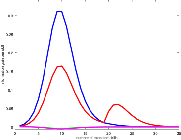
(a) Expected information gains for skills with simulated fingerprints $\mathbf{F}_{a_{1}}=(1,\,2)$ (blue), $\mathbf{F}_{a_{2}}=(2,\,4,\,5)$ (red), $\mathbf{F}_{a_{3}}=(3,\,4,\,6)$ (green, behind magenta), $\mathbf{F}_{a_{4}}=(3,\,4,\,5,\,6)$ (magenta). The skills $a_{3}$ and $a_{4}$ do not share any function with $a_{1}$, among which the error must be after executing $a_{1}$, and are ignored. For different executions of the algorithm the height and exact locations of the maxima might shift slightly due to the random generation of the fingerprint data.

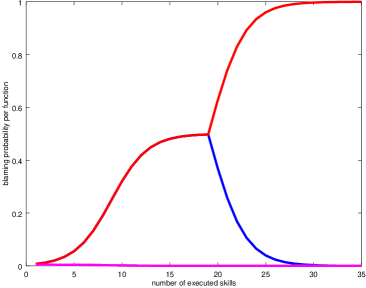
(b) $p_{\text{blame}}$ for the first 6 functions. All other functions have a low probability (comparable to the magenta curve) and are omitted. Initially the dominant skill is $a_{1}$ (cf. Fig. 2a), which cannot discriminate between functions $f_{1}$ (red) and $f_{2}$ (blue). After 19 steps, skill $a_{2}$ is chosen which identifies $f_{2}$ as the cause of error.

Figure 2: Typical information gains for four different skills and the respective probabilities $p_{\text{blame}}$ for functions 1 to 6 plotted over the number of executed skills. The function $f_{2}$ is simulated to be the cause of the error.

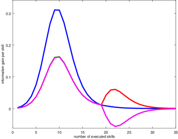
Figure 3: Expected information gains for skills with simulated fingerprints $\mathbf{F}_{a_{1}}=(1,\,2)$ (blue), $\mathbf{F}_{a_{2}}=(2,\,4,\,5)$ (red, hidden behind magenta), $\mathbf{F}_{a_{3}}=(1,\,3,\,6)$ (green, hidden behind magenta), $\mathbf{F}_{a_{4}}=(1,\,3,\,4,\,6)$ (magenta). As opposed to the scenario in Fig. 2a, the skills $a_{3}$ and $a_{4}$ can also help to identify the bug. The skills $a_{2}$ and $a_{3}$ are equally likely to be helpful and have the same expected information gain, whereas skill $a_{4}$ uses one function more than $a_{3}$ and therefore has a slightly lower expected information gain.

The probability $p_{dev}$ measures how much a measurement $\mu_{t_{\text{fail}}}^{\text{exec}}$ deviates from a regular execution of the skill $a$ within the time window $t\in\left[0,\,t_{\text{fail}}\right]$. Case 1 of equation 14 treats the case of a successful execution. The probability of observing a successful observation $o$ given the function $f_{i}$ has a bug should be low. However, a function might still have a bug but just did not affect the skill enough to make it fail. Therefore, $p_{a}\left(o\,|\,f=f_{i},\,\Delta_{a}\right)$ should increase if the finger print strongly differs from other successful experiences. The second case of equation 14 applies if the skill was not executed successfully. Each executed function should at least be suspicious, i.e. $p_{a}\left(o\,|\,f=f_{i},\,\Delta_{a}\right)\geq 1/2$. The probability increases proportionally to the deviation from previous successful experiences.

III-D Skill Selection by Information Gain Maximisation

The previous section described how to update the belief $p_{\text{blame}}\left(f=f_{i}\,|\,o_{1:T},o,\,a_{1:T},a\right)$ given a skill $a$ was selected. This skill should be selected such that the entropy of the probability distribution $p_{\text{blame}}$ decreases. A common way to solve this problem is to maximise the expected information gain. The information gain is defined by

$$I\left[a\right]=H\left[p_{\text{blame}}\left(f=f_{i}\,|\,o_{1:T},\,a_{1:T}\right)\right]-H\left[p_{\text{blame}}\left(f=f_{i}\,|\,o_{1:T},o,\,a_{1:T},a\right)\right]$$ (16)

Before executing the skill $a\in A$, the information gain cannot be computed directly, as the corresponding observation $o$ is not known yet. However, the current belief $p_{\text{blame}}\left(f=f_{i}\,|\,o_{1:T},\,a_{1:T}\right)$ can be used to estimate the expected information gain $\mathbf{E}\left[I\left[a\right]\right]$. We estimate $\mathbf{E}\left[I\left[a\right]\right]$ by uniformly sampling pairs $\left(succ,\,t_{\text{fail}}\right)$ for each sample in the database $\Delta_{a}$ with random success $succ\in\{\text{true},\,\text{false}\}$ and random failure time with probability $p(t_{\text{fail}})=1/T$. At each step a Bayesian belief update is performed, and the expected entropy $\mathbf{E}\left[H\left[p_{\text{blame}}\left(f=f_{i}\,|\,o_{1:T},o,\,a_{1:T},a\right)\right]\right]$ is estimated. The current entropy $H\left[p_{\text{blame}}\left(f=f_{i}\,|\,o_{1:T},\,a_{1:T}\right)\right]$ can be computed in closed form and the robot optimises

$$a_{\text{next}}=\operatorname*{arg\,max}_{a}{\mathbf{E}\left[I\left(a\right)\right]}=\operatorname*{arg\,max}_{a}{}\\ H\left[p_{\text{blame}}\left(f=f_{i}\,|\,o_{1:T},\,a_{1:T}\right)\right]-\mathbf{E}\left[H\left[p_{\text{blame}}\left(f=f_{i}\,|\,o_{1:T},o,\,a_{1:T},a\right)\right]\right].$$ (17)

IV Experiments

We evaluate our method in simulation and in real-world tasks. In simulation we analyse the behaviour of the Bayesian inference and the information gain optimisation independently of the MOM. Our approach is tested with a real robot by implementing a set of purposefully sabotaged skills.

IV-A Simulated Experiments

The Bayesian reasoning is decoupled from the MOM by generating artificial fingerprints of the type $\mathbf{F}_{a}\left(f_{1},\,f_{2},\,\dots\,f_{F}\right)=\left(\mathbf{fc}_{1},\,\mathbf{fc}_{2},\,\dots,,\,\mathbf{fc}_{F}\right)^{T}$. If $f_{i}=\text{false}$, the vector $\mathbf{fc}_{i}$ is chosen with $\mathbf{fc}_{i}=\vec{0}$. Otherwise it is given by $\mathbf{fc}_{i}=\left(fc_{i}(0)\propto\mathcal{N}(\mu_{i},\sigma_{i}),\,\dots,fc_{i}(T)\propto\mathcal{N}(\mu_{i},\sigma_{i})\right)^{T}$. If the matrices $\mathbf{F}_{a}\left(f_{1},\,f_{2},\,\dots\,f_{F}\right)$ are generated this way, the particular choice of the MOM is irrelevant. Artificial skills using the first 6 out of 241 available functions were generated. In order to simplify the notation, only used functions are denoted, e.g. $\mathbf{F}_{a}\left(\text{true},\,\text{true},\,\text{false},\,\dots,\,\text{false}\right)\equiv\mathbf{F}_{a}\left(1,\,2\right)$. In Figs. 2 – 4 typical evolutions of information gains and blaming probabilities by using skills with different fingerprints are shown. In all scenarios a bug in function $f_{2}$ causes an error if a skill uses $f_{2}$. Our system was able to detect the error in all scenarios with $p_{\text{blame}}(f=f_{2})\approx 1$. Fig. 2 shows a typical scenario, in which one skill is executed until another skill has a higher information gain. The skill is switched after 19 executions in order to discriminate between two failure candidates $f_{1}$ and $f_{2}$. Note that all functions except $f_{1}$ and $f_{2}$ have almost 0 probability as after executing the skill $a_{1}$ has identified that a bug must be in functions $f_{1}$ or $f_{2}$ which places the algorithm in a local optimum. If further bugs are contained in the software, the system has to be re-iterated when the bug in $f_{2}$ is fixed. The high number of functions with very low probability causes the probabilities in Fig. 2b to look like they are not normalised, however, this is just a visual artifact. Fig. 3 shows a similar scenario with a slightly different selection of used functions per skill. Even though the information gains develop differently, the bug belief develops the same way as in Fig. 2b because no different actions are taken. Fig. 4 shows a degenerate case in which two skills contribute equally much to identify the function $f_{2}$ and are executed alternately while the confidence in $f_{2}$ increases continuously. Even though the correct function is identified, the skill switching might require extra effort for preparation of different environments.

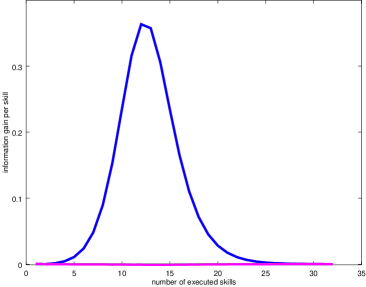
(a) Expected information gains for skills with simulated fingerprints $\mathbf{F}_{a_{1}}=(1,\,2)$ (blue), $\mathbf{F}_{a_{2}}=(2,\,4)$ (red, not visible, aligned with blue), $\mathbf{F}_{a_{3}}=(1,\,3,\,6)$ (green, not visible, aligned with magenta), $\mathbf{F}_{a_{4}}=(1,\,3,\,4,\,6)$ (magenta). Skills $a_{1}$ and $a_{2}$ have about the same expected information gain, which causes alternate execution.

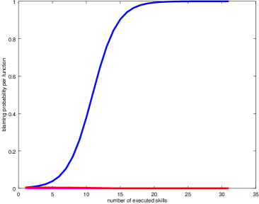
(b) The failure function is correctly identified early. The alternate execution of skills $a_{1}$ and $a_{2}$ yields a continuous improvement of confidence. All probablities excecpt for $f_{2}$ (blue) are close to 0.

Figure 4: Degenerate scenario: information gains for four different skills and the respective probabilities $p_{\text{blame}}$ for functions 1 to 6. The skills $a_{1}$ and $a_{2}$ are executed alternately. The function $f_{2}$ is simulated to be the cause of the error.

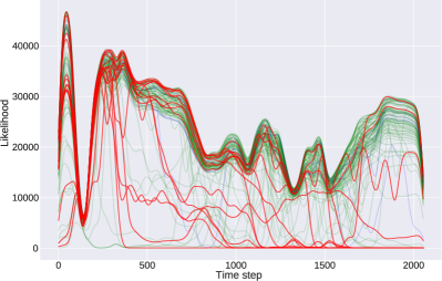
(a) Simple grasping skill

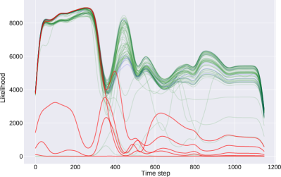
(b) Handover skill

Figure 5: MOM in two simple skill scenarios. The graphs show the reconstruction error likelihood over the execution time. It includes the (only positive) training samples (green), the positive test samples (blue) and the negative test samples (red). As can be seen, the method does not work in all cases, but the likelihood of a correct execution of a skill being classified as not working is relatively small.

IV-B Real-world experiments

We show the applicability of deep learning to failure detection in two simple tasks: simple grasping and object handover. Further, our system is tested with a set of simple skills by purposefully introducing bugs to the software. The robot setting used can be found in Fig. 6. It consists of two KUKA LWR 4+ robotic arms with one Schunk SDH gripper attached to each arm. The KUKA arms provide a control interface called fast research interface (FRI), which enables control and sensor data retrieval (joint positions, joint forces, Cartesian forces and torques). For object detection two Kinects are mounted - one on the chest and one above the robot. Objects are localised by segmenting them from the table surface and fitting a box to the remaining point cloud image by using PCL. Three different skills are implemented:

• Simple grasp: Objects are placed in front of the robot. A PCL based localiser recognises the objects and a Cartesian planner is used to move the end-effector. The fingers are closed and the object is lifted.

• Pressing a button: A red emergency button is placed in a fixed robot-relative position. A joint plan is executed and the button is pressed with the wrist and without using the fingers.

• Handover: The robot reaches forward by using a joint plan and waits until an object is placed in the hand. This event is detected by observing the end-effector forces. When an object is handed over, the fingers are closed.

IV-B1 Evaluation of the MOM

A set of erroneous executions was generated by either adding bugs to the code or by manually interfering with the environment, e.g. by kicking the object out of the robots hand.

Our implementation of the MOM uses a fully connected neural network with 32 output neurons and a RELU nonlinearity. The size of this bottleneck depends on the dimensionality of the input vectors. In our case, it was determined empirically. The GRU layer uses an internal $tanh$-nonlinearity and a logistic sigmoid nonlinearity for the output. The network is trained for 500 epochs which, on an nVidia GTX 1080 GPU for 70 sequences of 2000 time steps each, takes about five minutes.

Fig. 5a shows the MOM performance on the dataset for simple grasping. For most negative samples the likelihood of being a successful sample drops close to zero, while this is not the case for successful samples. Two different failure types are visible: the first failure type arises very early, at $t<500$, and corresponds to failed path planning which causes the arm not to move at all. When the arm moves, a failure cannot be detected as there is no contact with the object yet. Failures are detected when contact is made with the object from time $t>1000$. In the handover task (Fig 5b), the failure is detected when the arm does not move at all during the reaching motion or when the object should be placed in the hand, but is not. It should be noted that as soon as an error is detected, the further development of the reconstruction error is not relevant anymore.

IV-B2 Running the complete system

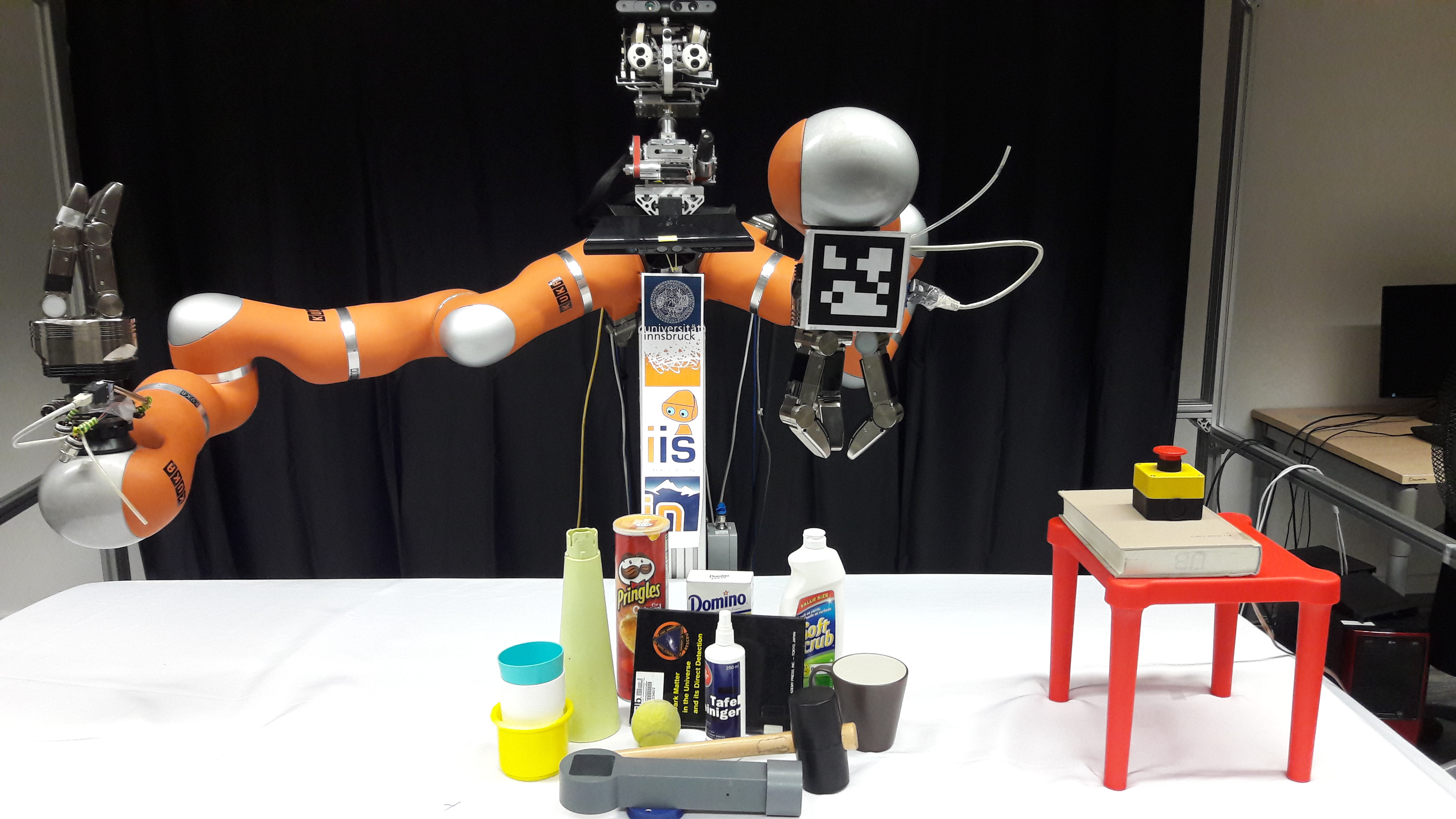
Figure 6: Robot setting and the used objects.

Sensor data and fingerprints were measured for at least 70 executions per skill. In total, more than 80 functions (including robot control) were used by the skills. Different types of bugs were purposefully introduced to the software. To reduce the computational effort for the estimation of the information gain, the decaying expected value in equation 12 was computed only for a window of 2 seconds before $t_{\text{fail}}$.

In the first scenario, the Cartesian planner was destroyed by introducing a constant shift. This type of error could happen if the robot model is not correct. The robot started to test the grasping skill which failed due to missing the object. It identified a set of potentially faulty functions and the 4 functions with the highest belief were {getRobotId, planJointTrajectory, storeJointInfoToDatabase, updateFilter}. None of these functions are related to the Cartesian shift bug. However, the confidence of the robot was low and planCartesianTrajectory was included with a similar probability. The grasping skill was used to confirm the belief until the button pressing skill provided a higher expected information gain. The button pressing skill was executed successfully because only a joint plan was used. This allowed the robot to exclude most wrong guesses and to suggest the list {cartesianPtp, planCartesianTrajectory, computeIk, closeHand} with high probability. The localiseObject is not suspicious as it was executed outside the time window, but is in the list as well if the window is enlarged. The handover skill enabled the robot to eliminate closeHand. All identified functions, i.e. {cartesianPtp, planCartesianTrajectory, computeIk}, are involved in Cartesian planning (and not in joint planning).

In the second scenario commands for moving the hand were not forwarded to the hardware. This affected the grasping skill and the handover skill, whereas the button pressing skill succeeded. All functions used in the button pressing skill were removed from the list of candidates (e.g. for joint planning, arm control functions) and the functions for Cartesian planning and hand control remained: {closeHand, cartesianPtp, planCartesianTrajectory, computeIk}. In the next step the handover skill was executed. Because the Cartesian planning functions were not used in the failing handover skill, the corresponding functions were eliminated.

In another scenario, the localisation system was destroyed by returning a constant position. In this case, the error is hard to detect: In the grasping scenario, the robot misses the object long after the localiser was run. If the time window is long enough, the system still identifies the localiser among other plausible candidates and returns the set {localiseObject, cartesianPtp, planCartesianTrajectory, computeIk} with high probabilities. Given the three provided skills, the robot has no possibility to discriminate between errors in the respective functions. In our setting, the localiser and Cartesian planning are always used together and an error in the localiser does not appear earlier in the sensor data. A video demonstration of the approach switching from one skill to another can be found online.

V Conclusion and Future Work

We introduced a skill-centric software testing approach that uses data collected over the life-time of a robot, which eliminates the need for defining separate test cases. We use two different types of data: sensor data of successful skill executions and corresponding profiling data. We train a so-called measurement observation model (MOM) (deep learning) and a functional profiling fingerprint (FPF) (Multivariate Gaussian model). Skills are executed as test cases and sensor data is compared to previous experiences. We use Bayesian belief updates to estimate a probability distribution of which functions contain bugs. The skills are selected in order to maximize the expected information gain. The approach is evaluated in simulation and in real robot experiments by purposefully introducing bugs to existing software.

This work discusses the problem of bug detection and autonomous testing. Future work will be concerned with developing autonomous strategies for bug fixing (e.g. by automatically performing selective git roll-backs or autonomously replacing hardware). Further, due to the lack of data, the likelihood function of the Bayesian belief update (equation 14) had to be hand-crafted following reasonable assumptions. In a more general framework the likelihood function can be trained automatically by providing ground truth data whenever the programmer has fixed a certain bug.

•

References

- [1] B. D. Argall, S. Chernova, M. Veloso, and B. Browning, “A survey of robot learning from demonstration,” Robotics and Autonomous Systems, vol. 57, no. 5, pp. 469 – 483, 2009. [Online]. Available: http://www.sciencedirect.com/science/article/pii/S0921889008001772
- [2] A. Cypher and D. C. Halbert, Watch what I do: programming by demonstration. MIT press, 1993.
- [3] S. Hangl, E. Ugur, S. Szedmak, A. Ude, and J. Piater, “Reactive, Task-specific Object Manipulation by Metric Reinforcement Learning,” in 17th International Conference on Advanced Robotics, 7 2015.
- [4] A. Bihlmaier and H. Wörn, Robot Unit Testing. Cham: Springer International Publishing, 2014, pp. 255–266.
- [5] J. Laval, L. Fabresse, and N. Bouraqadi, “A methodology for testing mobile autonomous robots,” in 2013 IEEE/RSJ International Conference on Intelligent Robots and Systems, Nov 2013, pp. 1842–1847.
- [6] J.-H. Lim, S.-H. Song, J.-R. Son, T.-Y. Kuc, H.-S. Park, and H.-S. Kim, “An automated test method for robot platform and its components,” International Journal of Software Engineering and Its Applications, vol. 4, no. 3, pp. 9–18, 2010.
- [7] G. Biggs, “Applying regression testing to software for robot hardware interaction,” in 2010 IEEE International Conference on Robotics and Automation, May 2010, pp. 4621–4626.
- [8] S. Zaman, G. Steinbauer, J. Maurer, P. Lepej, and S. Uran, “An integrated model-based diagnosis and repair architecture for ros-based robot systems,” in 2013 IEEE International Conference on Robotics and Automation, May 2013, pp. 482–489.
- [9] G. Steinbauer, F. Wotawa et al., “Detecting and locating faults in the control software of autonomous mobile robots.” in IJCAI. Citeseer, 2005, pp. 1742–1743.
- [10] S. Petters, D. Thomas, M. Friedmann, and O. von Stryk, Multilevel Testing of Control Software for Teams of Autonomous Mobile Robots. Berlin, Heidelberg: Springer Berlin Heidelberg, 2008, pp. 183–194.
- [11] J. R. Son, T. Y. Kuc, J. K. Park, and H. S. Kim, “Simulation based functional and performance evaluation of robot components and modules,” in 2011 International Conference on Information Science and Applications, April 2011, pp. 1–7.
- [12] H. S. Park and J. S. Kang, SITAF: simulation-based interface testing automation framework for robot software component. INTECH Open Access Publisher, 2012.
- [13] P. M. Frank and X. Ding, “Survey of robust residual generation and evaluation methods in observer-based fault detection systems,” Journal of process control, vol. 7, no. 6, pp. 403–424, 1997.
- [14] M. Hashimoto, H. Kawashima, and F. Oba, “A multi-model based fault detection and diagnosis of internal sensors for mobile robot,” in Intelligent Robots and Systems, 2003.(IROS 2003). Proceedings. 2003 IEEE/RSJ International Conference on, vol. 4. IEEE, 2003, pp. 3787–3792.
- [15] V. Verma, G. Gordon, R. Simmons, and S. Thrun, “Real-time fault diagnosis [robot fault diagnosis],” IEEE Robotics & Automation Magazine, vol. 11, no. 2, pp. 56–66, 2004.
- [16] K. L. Su, T. L. Chien, and C. Y. Liang, “Develop a self-diagnosis function auto-recharging device for mobile robot,” in IEEE International Safety, Security and Rescue Rototics, Workshop, 2005., June 2005, pp. 1–6.
- [17] D. Zhuo-hua, C. Zi-xing, and Y. Jin-xia, “Fault diagnosis and fault tolerant control for wheeled mobile robots under unknown environments: A survey,” in Proceedings of the 2005 IEEE International Conference on Robotics and Automation, April 2005, pp. 3428–3433.
- [18] J. Barata, L. Ribeiro, and M. Onori, “Diagnosis on evolvable production systems,” in 2007 IEEE International Symposium on Industrial Electronics, June 2007, pp. 3221–3226.
- [19] M. Yim, B. Shirmohammadi, J. Sastra, M. Park, M. Dugan, and C. J. Taylor, “Towards robotic self-reassembly after explosion,” in 2007 IEEE/RSJ International Conference on Intelligent Robots and Systems, Oct 2007, pp. 2767–2772.
- [20] K. Kawabata, S. Okina, T. Fujii, and H. Asama, “A system for self-diagnosis of an autonomous mobile robot using an internal state sensory system: fault detection and coping with the internal condition,” Advanced Robotics, vol. 17, no. 9, pp. 925–950, 2003.
- [21] M. H. Terra and R. Tinós, “Fault detection and isolation in robotic manipulators via neural networks: A comparison among three architectures for residual analysis,” Journal of Robotic Systems, vol. 18, no. 7, pp. 357–374, 2001. [Online]. Available: http://dx.doi.org/10.1002/rob.1029
- [22] T. Niemueller, G. Lakemeyer, and S. S. Srinivasa, “A generic robot database and its application in fault analysis and performance evaluation,” in 2012 IEEE/RSJ International Conference on Intelligent Robots and Systems, Oct 2012, pp. 364–369.
- [23] J. Rowley, “The wisdom hierarchy: representations of the dikw hierarchy,” Journal of information science, vol. 33, no. 2, pp. 163–180, 2007.
- [24] M. Sakurada and T. Yairi, “Anomaly detection using autoencoders with nonlinear dimensionality reduction,” in Proceedings of the MLSDA 2014 2nd Workshop on Machine Learning for Sensory Data Analysis. ACM, 2014, p. 4.
- [25] E. Marchi, F. Vesperini, F. Eyben, S. Squartini, and B. Schuller, “A novel approach for automatic acoustic novelty detection using a denoising autoencoder with bidirectional lstm neural networks,” in Acoustics, Speech and Signal Processing (ICASSP), 2015 IEEE International Conference on. IEEE, 2015, pp. 1996–2000.
- [26] K. Cho, B. Van Merriënboer, D. Bahdanau, and Y. Bengio, “On the properties of neural machine translation: Encoder-decoder approaches,” arXiv preprint arXiv:1409.1259, 2014.
- [27] D. Kingma and J. Ba, “Adam: A method for stochastic optimization,” arXiv preprint arXiv:1412.6980, 2014.
•