Calibration Of Proton Accelerator Beam Energy

Abstract

When studying the ${}^{7}Li\left(p,n\right)^{7}Be$ reaction with a RF accelerator, it is difficult to define the precise energy of the beam and its energy distribution, which together fully define the beam, for our purpose. What we do know is the difference between two given energies. We resolve this problem by finding a reference energy and then finding another energy by examining the data, relative to the reference energy. From the difference between them we can approximate the energy distribution for a given energy, and since we know the energy threshold of the reaction ($E_{threshold}$ for ${}^{7}Li\left(p,n\right)^{7}Be$ is about $1880.4-1880.8\>(keV)$) we can calibrate the beam energy. We then determine the energy which produce the maximum yield derivative as the reference and record the energy whose neutron yield is 5% of the reference energy. The data is collected by simulating this reaction using SimLit [1]. Since this is a simulation we know the real energy distribution so we make a linear fit for energy distribution as function of energy difference. We tested the theory on experimental data for which we approximate the energy distribution by other means, and found our new method to be accurate and satisfactory for our needs.

Racah Institute of Physics, The Hebrew University, Jerusalem, Israel, 91904

1 introduction

Our research uses a RF proton accelerator to produce ${}^{7}Li\left(p,n\right)^{7}Be$, and it is crucial to define the beam energy as accurately as we can. To do so we need the exact energy value and the energy spread (standard deviation), that from now on will be referred to as “energy sigma”. Although we don’t know the two values mentioned above, we do know the gap between any two energies the accelerator produces. Moreover, we can measure the number of neutron yield for a given angle with a Long Counter Detector. To solve our problem, we search for a well defined energy as a reference. By extracting this energy we can find another energy that conserves some relation value which we explain later on. After collecting these differences and their energy sigma we assume they fit each other linearly. Moreover we assume that the energy differences can point out the real value of the reference energy again by linear fit. This method is a new way to calibrate the proton beam energy. By putting in the equations the measured value of the energy difference extracted from a given experimental data, we can get the energy sigma and the real value of the reference energy (“new reference energy”). The rest is calibrated in reference to the new reference energy, since as we mentioned before we do know the gap between any two given energies. We tested this method and confirmed it on experimental data. Furthermore, we found that the angle contributions for this method in a Long Counter Detector are negligible.

2 methods

2.1 simulation with LiLiT

First we did simulation with SimLit at wide spectrum in terms of energies, angles, and energy sigma. Of ${}^{7}Li\left(p,n\right)^{7}Be$ reaction caused by accelerate protons on lithium target. The simulation sets we did where to take a constant energy spread and constant maximum angle, meaning we count all neutrons who scattered from the center of the target up to the maximum angle we determine. And we let the simulation to run on a rang of energies far less then the reaction threshold and up to 2 MeV. The simulation based on “Monte Carlo” that rely on repeated random sampling to compute their results. Verifying we make at least 10,000 events compensate the statistical error which is square rout of the samples number and to be as accurate as 1%. The data we extract were the excitation function and they look like figs (1) and (2).

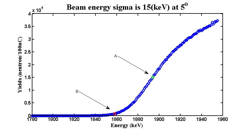
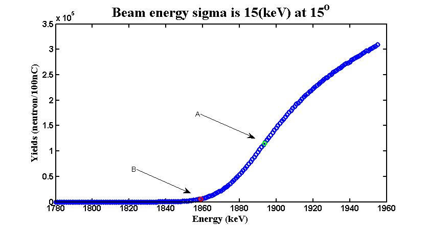
Figure 1: Example of neutron yield vs. energy. As plotted by SimLiT simulation at two differently angles - 5 and 15 degrees, between the direction of proton beam and the scattered neutron direction and the same energy spread. Point A in the graph is the reference energy as we extract from the derivative (shown in fig (3)) and point B is the energy that have 5% of the yield of point A. As can be observed the two graphs are almost similar, suggesting the that the angle dependent is negligible. Confirmed by many different sets of data.

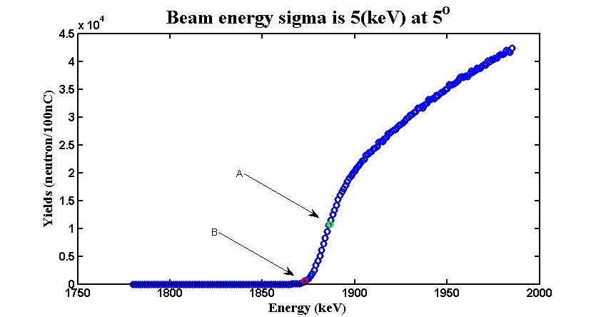
Figure 2: Example of neutron yield vs. energy. As plotted by SimLiT simulation at two differently energies spread - 5 and 15 keV and the same angle. Point A in the graph is the reference energy as we extract from the derivative (shown in fig (4)) and point B is the energy that have 5% of the yield of point A. As can be observed the two graphs are different. The reference energy shifted to an higher energy and the energy difference between the the two energies as grow bigger. Suggesting the that the energy spread and the real value of the reference energy are a characteristics variables of the problem. Confirmed by many different sets of data.

2.2 analysis of computed data

To find a uniquely defined energy in the excitation function (shown in fig (1)) we take the derivative of the this function (shown in fig (1)) and as can be seen we found a very distinct peak of yield density . We chose the energy that fits this peak as our reference energy. We define the lower energy as the energy which produces around 5% of the reference energy neutron yield. This act prevents noise interference. After doing so for several simulations we extract the values of the difference between the two energies in each experiment, and we know the energy sigma and the real value of the reference energy because this was a simulation. We did this analysis for different sets with the same statistics per cross section. From this data we extract a linear fit of energy sigma as a function of the gap, fig (5). And a linear fit of reference energy value as a function of the gap, fig (6).

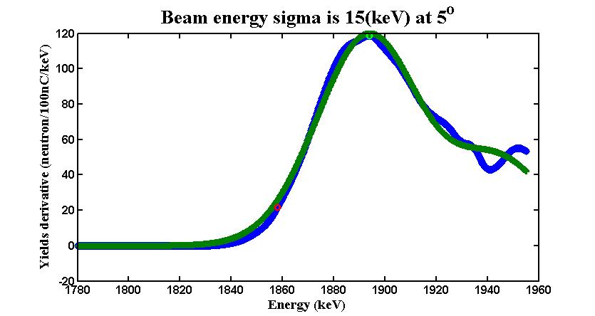
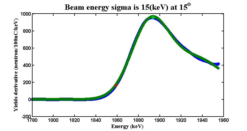
Figure 3: Example of the derivative of the excitation functions, fig (1). The blue graphs is the actual derivation and the green graph is fit of superposition of two gaussian, which give the best results for this method. The reference energy is the global maximum of the fit. As can be observed the two graphs are almost similar, suggesting the that the angle dependent is negligible. Confirmed by many different sets of data.

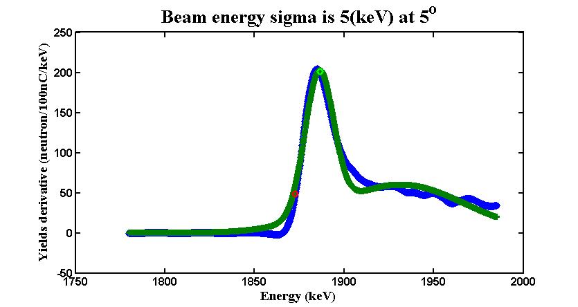
Figure 4: Example of the derivative of the excitation functions, fig (2). The blue graphs is the actual derivation and the green graph is fit of superposition of two gaussian, which give the best results for this method. The reference energy is the global maximum of the fit. As can be observed the two graphs are different. The reference energy shifted to an higher energy and the energy difference between the the two energies as grow bigger. Suggesting the that the energy spread and the real value of the reference energy are a characteristics variables of the problem. Confirmed by many different sets of data.

2.3 the data from the simulation

index	energy sigma	low energy	reference energy	energy difference
1	1	1876.2	1884.4	8.2
2	2	1875.8	1884.4	8.6
3	3	1875	1885	10
4	4	1874	1885.6	11.6
5	5	1872.8	1886.4	13.6
6	6	1871.6	1887.2	15.6
7	7	1870	1887.8	17.8
8	8	1868.6	1888.6	20
9	9	1867	1889.2	22.2
10	10	1865.6	1890.2	24.6
11	11	1863.8	1890.4	26.6
12	12	1862	1891	28.6
13	13	1861	1891.8	30.8
14	14	1859.2	1892	32.8
15	15	1858	1894	36
16	16	1856	1893	37
17	17	1854.4	1894	39.6
18	18	1853	1894.6	41.6
19	19	1851.4	1895.2	43.8
20	20	1849.8	1895.6	45.8

Table 1: The data from SimLiT simulation at 5 degrees. Energy’s value presented in keV. The data ploted on figs (5),(6).

index	energy sigma	low energy	reference energy	energy difference
1	1	1877.2	1886	8.8
2	2	1876.8	1886.2	9.4
3	3	1876.2	1886.8	10.6
4	4	1875.2	1887.4	12.2
5	5	1874	1888	14
6	6	1872.6	1888.6	16
7	7	1871.2	1889.4	18.2
8	8	1869.8	1890	20.2
9	9	1868.2	1890.8	22.6
10	10	1866.8	1891.2	24.4
11	11	1865.2	1891.6	26.4
12	12	1863.6	1892	28.4
13	13	1862	1892.8	30.8
14	14	1860.6	1893.4	32.8
15	15	1858.8	1893.6	34.8
16	16	1857.2	1894.2	37
17	17	1855.6	1894.6	39
18	18	1854.2	1895.4	41.2
19	19	1852.6	1896.2	43.6
20	20	1851	1896.6	45.6

Table 2: The data from SimLiT simulation at 15 degrees. Energy’s value presented in keV. The data ploted on figs (5),(6).

Here is the function that we extracted :

$$\sigma(\vartriangle E)=0.463\bullet\vartriangle E-1.3$$ (1)

$$E_{reference}(\bigtriangleup E)=0.289\bullet\bigtriangleup E+1883$$ (2)

And this is plot of the data with their fit.

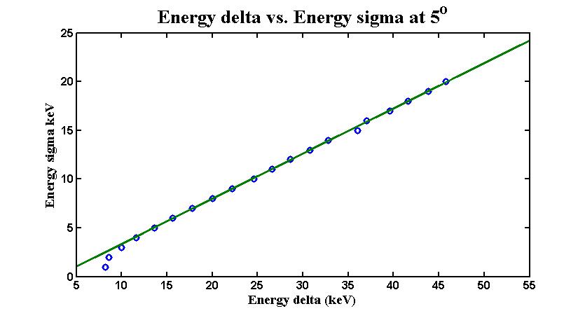
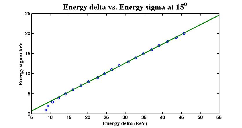
Figure 5: The graph represent the data of the energy gap between the reference energy and the low energy vs the known energy spread. As extract from SimLiT simulation. The grin graph is the linear fit we suggested. As can be seen our fit is not accurate at small values of energy gap, smaller than 10 keV. At thous energy gaps we can estimate by other means and we do not relay on our method. In contrary at high energy spread our method is fit very well and it can use as analysis tool. Moreover we can see that the two fits at different angles aren’t differ from each other. Confirming that the angle dependent is negligible.

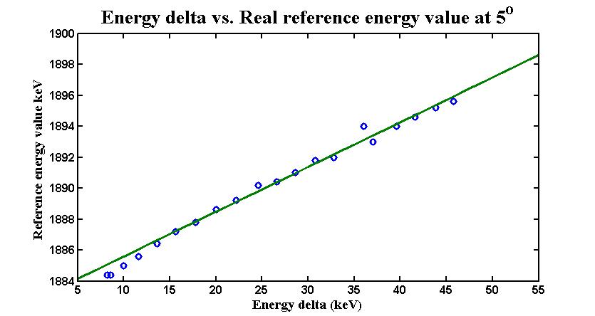
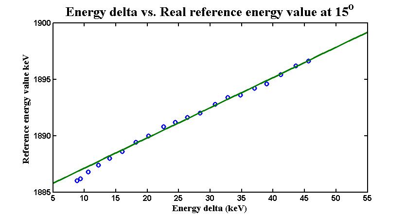
Figure 6: The graph represent the data of the energy gap between the reference energy and the low energy vs the known real value of the reference energy. As extract from SimLiT simulation. The grin graph is the linear fit we suggested. As can be seen our fit is not accurate at small values of energy gap, smaller than 15 keV. At thous energy gaps we can estimate by other means and we do not relay on our method. In contrary at high energy spread our method is fit very well and it can use as analysis tool. Moreover we can see that the two fits at different angles aren’t differ from each other. Confirming that the angle dependent is negligible.

2.4 using those fits to calibrate experimental data

Assuming this phenomena is an continues phenomena. We can imagine that if we do the same analysis on a real experimental data, who done approximately at the same conditions. We will get a value for the gap between the high energy and the low one. Now instead of making a set of points we gust put the energy gap in the fit we gust mentioned, and extract the energy spread an the real absolute value of the reference energy. This method doesn’t take in to account any physical dimensions of the problem, and it doesn’t use any absolute value of the problem but the peak at the derivative function which is a characteristic of the problem.

3 results

Our results as we extracted from the data by these means are shown here, we present three different data sets, that we estimated the energy sigma and the shift of the energy axis, using our new method and other methods for cooperation.

First data set we approximate sigma to be 1.5keV while the new method shows.

$$\sigma(\vartriangle E=2.6\>(keV))=0.463\bullet 2.6-1.3=-0.096\>(keV)$$ (3)

$$E_{reference}(\bigtriangleup E=2.6\>(keV))=0.289\bullet 2.6+1883=1883.4\>(keV)$$ (4)

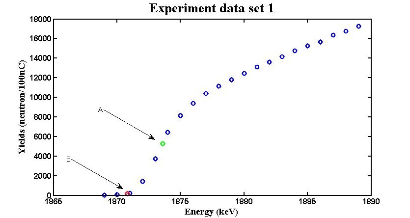
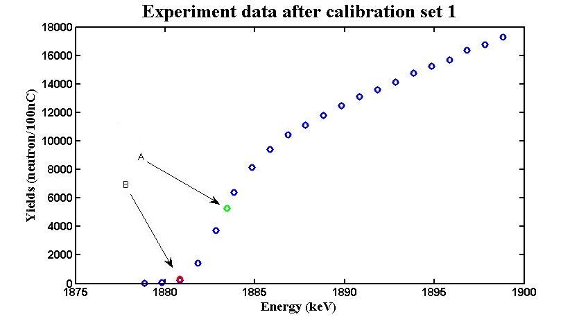
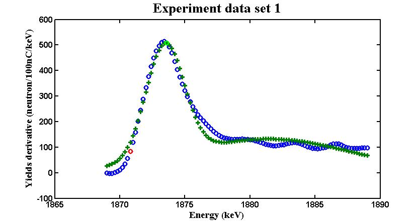
Figure 7: Example of real experiment analysis of data set [2] with narrow energy sigma. Point A in the graph is the reference energy as we extract from the derivative (third graph in this data set) and point B is the energy that have 5% of the yield of point A. The first graph is the yield of neutrons counted by long counter detector time normalized, and the energies is the energies the accelerator measured before it hit the target. The second graph is the same as the first one after calibration of the energy axis with our new method. At the third graph the blue graphs is the actual derivation and the green graph is fit of superposition of two gaussian, which give the best results for this method. The reference energy is the global maximum of the fit. Exact values can be seen at table (3).

Second data set our approximation sigma is 15keV while the new method shows.

$$\sigma(\vartriangle E=55.4\>(keV))=0.463\bullet 55.4-1.3=24.37\>(keV)$$ (5)

$$E_{reference}(\bigtriangleup E=55.4\>(keV))=0.289\bullet 55.4+1883=1898.7\>(keV)$$ (6)

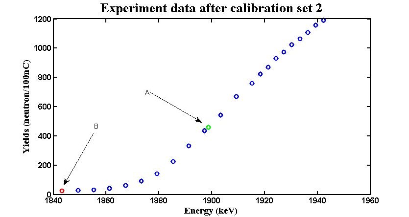
Figure 8: Example of real experiment analysis of data set [3] with wide energy sigma. Point A in the graph is the reference energy as we extract from the derivative (third graph in this data set) and point B is the energy that have 5% of the yield of point A. The first graph is the yield of neutrons counted by long counter detector time normalized, and the energies is the energies the accelerator measured before it hit the gold foil, which spread the energy to a wide spectra. The second graph is the same as the first one after calibration of the energy axis with our new method. At the third graph the blue graphs is the actual derivation and the green graph is fit of superposition of two gaussian, which give the best results for this method. The reference energy is the global maximum of the fit. Exact values can be seen at table (3).

Third data set our approximation sigma is 20keV and shift of keV while the new method shows.

$$\sigma(\vartriangle E=53.2\>(keV))=0.463\bullet 53.2-1.3=23.35\>(keV)$$ (7)

$$E_{reference}(\bigtriangleup E=53.2\>(keV))=0.289\bullet 53.2+1883=1898.1\>(keV)$$ (8)

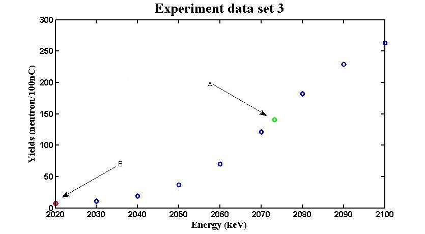
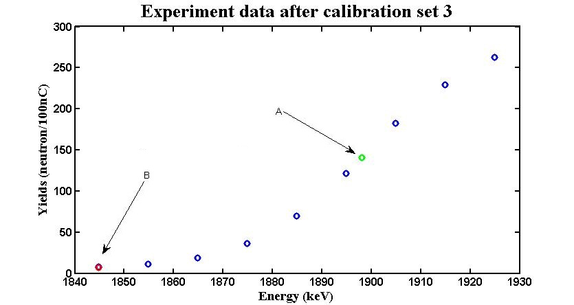
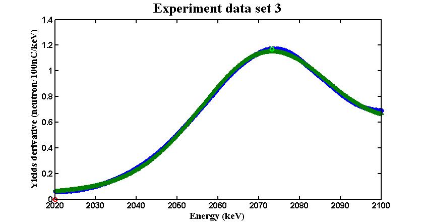
Figure 9: Example of real experiment analysis of data set [4] with wide energy sigma. Point A in the graph is the reference energy as we extract from the derivative (third graph in this data set) and point B is the energy that have 5% of the yield of point A. The first graph is the yield of neutrons counted by long counter detector time normalized, and the energies is the energies the accelerator measured before it hit the gold foil, which spread the energy to a wide spectra. The second graph is the same as the first one after calibration of the energy axis with our new method. At the third graph the blue graphs is the actual derivation and the green graph is fit of superposition of two gaussian, which give the best results for this method. The reference energy is the global maximum of the fit. Exact values can be seen at table (3).

all the data as we extract can be seen at table (3).

index	energy sigma	low energy	reference energy	energy difference	energy sigma*	reference energy value*
1	1.5	1871	1873.6	2.6	-0.1	1882.1
2	15	2015	2070.4	55.4	24.37	1899
3	20	2020	2073.2	53.2	23.35	1898

Table 3: The data from the real experiment,which extracted by the same means as at the simulations. Energy’s value presented in keV

4 summary

As we said this method doesn’t take in to account any physical dimensions of the problem. Which make it an independent new way to analysis of the experimental data.

To use this method do the following:

• Fit your data as good as you can.

• Derive this fit and find the energy that gives the maximum.

• Find the neutron yield at that energy.

• Find the energy at which you measured 5% yield.

• Subtract one from the other and take the absolute value; this value is $\vartriangle E$.

• To find your approximate energy distribution use equation (1) as shown in equations (3) and (5).

• Change the energy value of the high energy according to equation (2) and change the axis values with the same scale as before, now using the new energy as reference point.

VERY IMPORTANT - make sure the low energy yield value is more than 5% !!! else you need to extract the fits for the sigma energy and the real value of reference energy, referring to the minimum present you can get from the specific data. our fits is relevant for long counter detector and thick lithium target.

References

- [1] M. Friedman, G. Feinberg, D. Berkovits, Y. Eisen, M. Paul, A. Shor, Neutron Spectrum of Liquid-Lithium Target at Soreq Applied Research Accelerator Facility, to be published
- [2] Log book I page 22, threshold scan target , 16-3-2010
- [3] Log book I page 68, threshold scan target with gold foil, 24-3-2010
- [4] Log book II page 15, target B1,