Prowess - a software model for the Ooty Wide Field Array

Abstract

One of the scientific objectives of the Ooty Wide Field Array(OWFA) is to observe the redshifted Hi emission from $z\sim 3.35$. Although predictions spell out optimistic outcomes in reasonable integration times, these studies were based purely on analytical assumptions, without accounting for limiting systematics. A software model for OWFA has been developed with a view to understanding the instrument-induced systematics, by describing a complete software model for the instrument. This model has been implemented through a suite of programs, together called Prowess, which has been conceived with a dual role of an emulator as well as observatory data analysis software. The programming philosophy followed in building Prowess enables any user to define an own set of functions and add new functionality. This paper describes a co-ordinate system suitable for OWFA in which the baselines are defined. The foregrounds are simulated from their angular power spectra. The visibilities are then computed from the foregrounds. These visibilities are then used for further processing, such as calibration and power spectrum estimation. The package allows for rich visualisation features in multiple output formats in an interactive fashion, giving the user an intuitive feel for the data. Prowess has been extensively used for numerical predictions of the foregrounds for the OWFA Hi experiment.

1 Introduction

One of the principal aims of the upgrade of the Ooty Radio Telescope (ORT) to OWFA(Prasad & Subrahmanya, 2011; Subrahmanya, Manoharan & Chengalur, 2017; Subrahmanya et al., 2017) is to enable the detection of Hi emission from large scale structures in the post-EoR universe at redshifts $\sim 3$. Theoretical calculations of the expected emission tuned to the projected parameters of OWFA indicate that the telescope should have sufficient sensitivity to detect the power spectrum of the redshifted Hi 21-cm emission, in integration times of a few hundred hours(Ali & Bharadwaj, 2014; Bharadwaj, Sarkar & Ali, 2015; Sarkar, Bharadwaj & Ali, 2017). Currently, a number of experiments are in various stages of progress that aim to directly detect the brightness temperature fluctuations $\delta T_{b}$ of the 21-cm post-reionisation cosmological signal like the Canadian Hydrogen Intensity Mapping Experiment (CHIME; Bandura et al. 2014), Baryon Acoustic Oscillation Broadband and Broad-beam Array (BAOBAB; Pober et al. 2013) and the Tianlai Cylinder Radio Telescope (CRT; Chen 2011; Xu, Wang & Chen 2015). These experiments would each operate at different frequency ranges; BAOBAB has been proposed to specifically detect the Baryon Acoustic Oscillation (BAO) feature in the redshifted Hi 21-cm line in the 600-900 MHz band. The Tianlai CRT also is gearing up to detect the BAO features and constrain dark energy through redshifted Hi 21-cm observations in the 700-1400 MHz band(Chen, 2011; Xu, Wang & Chen, 2015). CHIME would overlap with both these experiments in the range $\sim 400-800$ MHz. The OWFA cosmology experiment is expected to fill a significant gap in understanding the evolution of post-reionisation neutral hydrogen at large scales in an important redshift interval of $z\sim 3.35$.

While the raw sensitivity of the telescope would be sufficient to detect the Hi emission from redshifts $z\sim 3.35$(Ali & Bharadwaj, 2014; Bharadwaj, Sarkar & Ali, 2015), the expected signal is many orders of magnitude fainter than the other astrophysical signals, i.e. the “foregrounds”(see e.g. Santos, Cooray & Knox, 2005; Ali, Bharadwaj & Chengalur, 2008). These include emission from the diffuse ionised galactic interstellar medium (“diffuse Galactic synchrotron emission” and “galactic free-free emission”) and emission from the extragalactic radio sources(called “the extragalactic foreground”) that the telescope is sensitive to. Many instrumental effects come into play when the signal of interest is buried several in orders of magnitude brighter foregrounds: systematics introduced by uncalibrated antenna gains, interference from terrestrial sources and effects of the complex intrinsic interaction between the instrument and the foregrounds, due to the chromatic response of the telescope, are thought to be the dominant contributors. A good understanding of all of these issues is required to enable a robust prediction of the cosmological signal that could be detected through observations with OWFA.

The first step to understanding the instrumental systematics is to develop a thorough understanding of the instrument itself, and capture it in a software model that would include all the expected instrumental effects. All of the astrophysical signals(e.g. the diffuse Galactic and the extragalactic point source foregrounds) can then be suitably parametrized and included in the model. One of the expected by-products of the exercise to detect the cosmological Hi signal is a better understanding of some of the foregrounds, particularly of the diffuse Galactic foreground, which is the dominant foreground from within the Galaxy and of interest in itself(see e.g. Iacobelli, Haverkorn & Katgert, 2013; Iacobelli et al., 2013, 2014). The ability to characterise the foregrounds and the fundamental limitations set by the instrument are both crucial to enable realistic predictions for the redshifted Hi 21-cm detection. The software model described in this paper was developed in order to help better understand the systematics, as well as devise methods to devise foreground characterisation and subtraction methods.

2 The rationale for a software model

The OWFA Hi experiment is a challenging one in terms of both the special hardware requirements as well as the methods and algorithms that eventually enable us to measure the Hi power spectrum. A significant component of the design of an experiment, especially in modern low frequency radio cosmology, has been the investment in simulating the instrument and the experiment itself based purely on a software model. The results from simulations can often influence the course of the experiment through valuable insight. This has been the driving philosophy for an emulator based on a software model for the OWFA Hi experiment.

For OWFA, traditional interferometric data analysis software packages are not useful as they do not provide sufficient functionality for redundancy calibration, or for the final processing which, in this case, is not imaging. A complete software suite has been developed consisting of several standalone programs that serve two simultaneous purposes:

• to simulate visibilities as obtained from OWFA, based on the instrument and sky description. The instrument description should naturally lead to all the effects and systematics that are expected to be present in an actual interferometric observation. Simulated data can provide a test bed for devising and refining RFI mitigation algorithms, calibration algorithms and statistical estimators for signal characterisation, etc.

• to function as the observatory software pipeline that is used to process real data from the telescope, so that the simulations above inform us to refine and adopt the optimal strategies for working with real data.

Given that a software model for the telescope and the sky would serve as a very useful guide to the experiment, I shall now set up the preliminaries for describing the emulator in some detail, and list its various features with examples.

3 The programming philosophy

The software suite that has been developed for OWFA simulations is a C-based collection of utilities and algorithm implementations. Visualisation of data is almost the first step in data handling and a standard format definition should therefore be the first choice. The suite was conceived from the early days as one that would grow organically to accommodate observatory needs. Therefore, the choice was to adhere to an international standard for the visibility data, so that a team of astronomers stationed in widely separated geographical locations can handle these data using this software suite. The following considerations were kept in mind during the development of the emulator.

• The Flexible Image Transport System(FITS; Wells, Greisen & Harten 1981) or the Measurement Set(MS; Kemball & Wieringa 2000) format definitions were the obvious formats to choose from. The fact that FITS is the data format at the GMRT and hence is familiar to astronomers both within NCRA and users of the GMRT played a significant role in the decision to adopt it. However, it is worth mentioning that the Hierarchical Data Format (HDF) (see e.g. Price, Barsdell & Greenhill, 2015, for advantages of HDF5 over UVFITS) could be considered in the future due to its advantages over FITS, such as compressibility and parallel I/O. The availability of conversion libraries from FITS to HDF5 makes this an attractive alternative if the full potential of parallel processing is to be harnessed. Pre-conversion of UVFITS observatory data to HDF5 is then the only extra step in the offline processing necessitated by this choice. UVFITS will therefore currently remain the observatory data format of choice.

• The second major factor was the ability to add new utilities to the suite by anyone familiar with the FITS definition. Therefore, the suite comes with a very rich set of subroutine functions that do standard operations in a transparent manner. A new utility that has to operate on the FITS data at the level of individual records can hence draw on this library of subroutines.

• Finally, a high level of ease with which utilities can be added to the suite is achieved by making the chore of passing arguments to function calls a trivial operation. Instead of passing specific arguments to functions, the pointer to a global superstructure is passed uniformly to all function calls. The superstructure itself is a structure of many structures, which are defined in different header files depending on their functionality. Therefore, any user would be able to add her own function definition to the existing subroutines by passing a single argument.

Figure 1 captures the spirit of the programming philosophy. The main call merely initialises a few variables specific to the program.

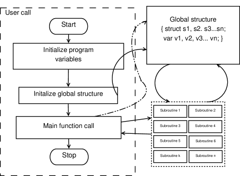
Figure 1: The general model for each program in the OWFA simulator suite

Subroutines, variables and structures are segregated according to their functionality and defined in appropriate header files. Similarly, subroutine functions are defined in functionally separable C program files. For example, all function definitions related to the instrument are available in the inc/sysdefs.h and src/syssubs.c files. FITS-related definitions and structures are to be found in inc/fitsdefs.h and src/fitssubs.c files. Sky simulations are grouped under inc/skydefs.h and src/skysubs.c. Mathematical function definitions and structures are grouped under inc/matdefs.h and src/matsubs.c. The global superstructure, which holds all the variables and structures is defined to be of type ProjParType, which is defined in inc/sysdefs.h.

4 Prowess - a Programmable OWFA Emulator System

The software suite is given the name “Programmable OWFA Emulator System”, and it is self-explanatory. Programmable, because adding new utilities or functionality is made easy as described in the previous section, and the emulator is specific to OWFA. I shall now describe the preliminaries required to capture the instrument in a software model.

4.1 Antennas and baselines

OWFA(Subrahmanya, Manoharan & Chengalur, 2017; Subrahmanya et al., 2017) would operate in two concurrent modes - Phase-I and Phase-II. Phase-I is a 40-antenna interferometer and Phase-II is a 264-antenna interferometer. Only Phase-II refers to an operational system and Phase-I is achieved in software. The Ooty Radio Telescope(ORT) is a $\sim 530$ m long cylinder that is 30 m wide(Swarup et al., 1971). The telescope consists of 1056 dipoles arranged regularly along its length. These 1056 dipoles are grouped into 22 modules, each module being supported mechanically by a parabolic frame. All the 22 frames are steered in unison through a common drive shaft. Each of the 22 modules is the sum of a contiguous group of 48 dipoles, combined through a passive combiner network. The signals from the dipoles are summed hierarchically, and the second smallest unit in this hierarchy is the output of the 4-way combiner(Subrahmanya et al., 2017). The signals from six Phase-II apertures are again summed in two stages to give the Phase-I aperture. Correspondingly, the two interferometer modes provide two different aperture settings:

• The output of the 4-way combiner forms the aperture of the Phase-II system. Every group of 4 dipoles, or a sixth of a half-module, would operate as a single element in Phase-II. This corresponds to 1.92 m of the 530 m long cylinder, equivalent to 2$\lambda$. This results in 264 apertures throughout the length of the telescope.

• The output of the sum of six 4-way combiners forms the aperture of the Phase-I system, equivalent to one half-module. Therefore, every group of 24 dipoles would operate as a single element in Phase-I. This corresponds to 11.5 m of the 530 m long cylinder, equivalent to 12.5$\lambda$. This results in 40 apertures throughout the length of the telescope.

#AntIdΨ   AntΨ    bxΨ    by      bz     ddly    fdly
#------------------------------------------------------------
ANT00Ψ   N10NΨ   0.0    0.0    10.0Ψ     0.0     0.0
ANT01Ψ   N10SΨ   0.0Ψ   0.0    21.5Ψ     0.0Ψ    0.0
.        .       .      .      .         .       .
.        .       .      .      .         .       .
.        .       .      .      .         .       .
ANT38Ψ   S10NΨ   0.0Ψ   0.0Ψ  447.0Ψ     0.0Ψ    0.0
ANT39Ψ   S10SΨ   0.0Ψ   0.0Ψ  458.5      0.0Ψ    0.0
#END

Figure 2: The antenna definition file Antenna.Def.40 for Phase-I of the OWFA interferometer.

To begin with, the emulator has to be initialised with the antenna positions. This is done through an input Antenna Definition file, “Antenna.Def.40” for Phase-I and “Antenna.Def.264” for Phase-II. The parsing section of the code then figures out which of the two modes the telescope is being operated in. Accordingly, it sets the aperture dimensions. The user has the option to switch off certain antennas in the “Antenna.Def” file to simulate a situation when some antennas are not available. These are then omitted from the simulations as well as the output visibility data. This not only obviates the need to maintain a running log of the invalid antennas, but also eases memory and storage requirements. Figure 2 shows the antenna definition for Phase-I. The file has seven columns:

1. Column 1 shows the antenna identifier used by the FITS standard.

2. Column 2 is the antenna name; the name of each antenna is tied to its identifier. This helps in unambiguous bookkeeping even when switching off certain antennas.

3. Columns 3, 4 and 5 respectively give the antenna $x,y$ and $z$ co-ordinates in a right-handed co-ordinate system, which shall be described shortly.

4. Columns 6 and 7 respectively denote the delay in seconds, corresponding to the number of integer and fractional clock cycles offset with respect to a reference antenna. At the moment, these fields are not being used, hence their values are all set to zero. In practice, these would represent the fixed delays arising from differences in cable lengths.Therefore they can be measured reasonably accurately and are unlikely to change in an undisturbed setup. These fields would be used to correct for the phase ramps in the visibilities across the band for each baseline.

Since the dipoles are regularly spaced, the equivalent apertures in Phase-I and Phase-II are also regularly spaced. This results in an interferometer in which the separation between any pair of apertures is an integral multiple of the shortest separation between adjacent apertures,

$$d_{\mathrm{n}}=nd$$ (1)

where $d$ is the both the size of the aperture as well as the shortest spacing. The 40-antenna Phase-I has twenty half-modules in the northern half and twenty in the southern half. The northern ones are named N01 to N10 outwards from the midpoint of the telescope, and similarly the southern modules. The two half-modules within each module are given a “N” or “S” identifier. The antenna definition file is parsed and the values are stored in the antenna structure within the superstructure(ProjParType).

In the co-ordinate system chosen for OWFA, the antennas are placed along the $z$-axis.

###  Antenna  ΨRe(gain)   ΨIm(gain)    abs(gain)    arg(gain)
###
 0   ΨN10N   Ψ 2.111527   -1.651020   Ψ2.680375   Ψ-38.022146
 1   ΨN10S   Ψ-0.769040    2.448255    2.566198   Ψ107.438412
 .    .        .           .           .            .
 .    .        .           .           .            .
 .    .        .           .           .            .
38   ΨS10N   Ψ 0.112905    1.564518    1.568587   Ψ 85.872353
39   ΨS10S   Ψ 1.386609   -1.809840   Ψ2.279958   Ψ-52.542475

Figure 3: The antenna initialiser log, with the complex gain assigned to each antenna.

Each antenna $i$ is assigned a complex, frequency dependent, electronic gain $g_{i}$, obtained as a random complex number distributed around a mean gain $|g|$, referred to the central frequency $\nu_{0}$ = 326.5 MHz. The observing band is split into $N$ channels. It is possible to introduce slowly time-varying gains in the simulations about the mean antenna gains described above, but such gain variations are automatically handled at the time of calibration.

###Ψ   Ant1  Ant2  Ψ FITSbl  Ant1    Ant2
###
  1   Ψ 0   Ψ 1   Ψ   257   ΨN10N   ΨN10S
  2   Ψ 0   Ψ 2   Ψ   258   ΨN10N   ΨN09N
  .     .     .       .      .       .
  .     .     .       .      .       .
  .     .     .        .     .       .
 38   Ψ 0   Ψ38   Ψ   294   ΨN10N   ΨS10N
 39   Ψ 0   Ψ39   Ψ   295   ΨN10N   ΨS10S

Figure 4: The log “baselines.info” that lists the baselines counted as pairs of the available antennas. Only the first 39 baselines of Phase-I are shown as an example.

The antenna structure initialization information is written out in a log called “ant-init.info”. The real and imaginary parts of the complex gains, as well as its amplitude and phase(in degrees) at $\nu_{0}$ are written out in the file. An example is shown in Figure 3.

Baselines are then obtained as antenna pairs, and each baseline is written into a structure that holds the baseline number, the participating antenna pair, the three dimensions of the baseline and its length in wavelength units at the reference frequency. A log of the baselines is written out to “baseline.info”, part of which is shown in Figure 4. An $N_{A}$ antenna interferometer results in ${}^{N_{A}}C_{2}$ baselines, giving 780 for Phase-I and 34716 for Phase-II. The baseline vectors are obtained from the physical antenna separations, defined at the central frequency $\nu_{0}$ but at each channel it is appropriately scaled when computing the visibilities.

$$\mathbf{d}_{|a-b|}=\mathbf{x}_{a}-\mathbf{x}_{b}$$ (2)

$$\mathbf{U}_{|a-b|}=\mathbf{d}_{|a-b|}\ \frac{\nu}{c}$$ (3)

Equation 2 shows the physical separation between antenna pairs, whereas equation 3 shows the baseline in wavelength units at any given frequency $\nu$. The regular spacing of the antennas results in baselines with redundant spacings. As a result, we obtain $N_{A}-n$ copies of the baseline with a separation of $n$ units. In this case of an $N_{A}$-antenna linear array, only $N_{A}-1$ baselines out of ${}^{N_{A}}C_{2}$ are unique and non-redundant. All of these $N_{A}-1$ baselines have redundant copies, except the longest one.

4.2 A co-ordinate system suitable for OWFA

A generalised framework for computing the visibilities is presented here. Consider a right-handed Cartesian coordinate system, shown in Figure 5, tied to the telescope, in which the $z$-axis is along the N-S direction, parallel to the axis of the parabolic cylinder, the $x$-axis is aligned with the normal to the telescope aperture which is directed towards $(\alpha_{0},0)$ on the celestial equator, and the $y$ axis is in the plane of the telescope’s aperture, perpendicular to both the $x$ and $z$ axes respectively. $\mathbf{\hat{i}},\mathbf{\hat{j}}$ and $\mathbf{\hat{k}}$ denote the

Figure 5: A schematic of the co-ordinate system for computing the visibilities, in which $\mathbf{n}$ is an arbitrary direction and $\mathbf{m}$ is the direction of pointing. The visibilities are computed over the entire solid angle of the celestial hemisphere.

unit vectors along $x,y$ and $z$. In this coordinate system, we have

$$\mathbf{U}=v\mathbf{\hat{k}}$$ (4)

Observations are centered on a position $(\alpha_{0},\delta_{0})$ on the celestial sphere: let the unit vector $\mathbf{\hat{m}}$ denote this position on the celestial sphere. $\mathbf{\hat{m}}$ always lives on the $x\!-\!z$ plane, and is given by

$$\mathbf{\hat{m}}=\sin(\delta_{o})\,\mathbf{\hat{k}}+\cos(\delta_{0})\,\mathbf{\hat{i}}$$ (5)

The measured visibility for a baseline of length $\mathbf{U}$ at a frequency $\nu$ can be written as

$$\mathbf{M}(\mathbf{U},\nu)=\int d\Omega_{\mathbf{\hat{n}}}\,I(\mathbf{n},\nu)\,A(\Delta\mathbf{n},\nu)\,e^{2\pi i\mathbf{U}\cdot\Delta\mathbf{n}}$$ (6)

where $\mathbf{\hat{n}}$ refers to an arbitrary direction in the celestial sphere, given by

$$\mathbf{\hat{n}}=\sin(\delta)\,\mathbf{\hat{k}}+\cos(\delta)\left[\cos(\alpha-\alpha_{0})\,\mathbf{\hat{i}}+\sin(\alpha-\alpha_{0})\mathbf{\hat{j}}\right]$$ (7)

The solid angle integral here is over the entire celestial hemisphere, and

$$\Delta n=\mathbf{\hat{n}}-\mathbf{\hat{m}}$$ (8)

We finally have

$$\mathbf{M}(\mathbf{U},\nu)=\int[d\sin(\delta)\,d\alpha]\,I(\alpha,\delta,\nu)\,e^{2\pi iv[\sin(\delta-\delta_{0})]}A(\Delta n_{y},\Delta n_{z})$$ (9)

where $\Delta n_{y}=\cos(\delta)\,\sin(\alpha-\alpha_{0})$ and $\Delta n_{z}=\sin(\delta-\delta_{0})$. Note that in this co-ordinate system the argument of the exponent depends only on the baseline length and the declination, reflecting the 1D geometry of OWFA.

4.3 Aperture and the primary beam

We may write the general beam pattern for a rectangular aperture as $A(\Delta\mathbf{n})\equiv A(\Delta n_{y},\Delta n_{z})$ where $(\Delta n_{y},\Delta n_{z})$ are respectively the $y$ and $z$ components of $\Delta\mathbf{n}$. The Phase-I aperture is $11.5\mathrm{m}\times 30\mathrm{m}$ and the Phase-II aperture is $1.92\mathrm{m}\times 30\mathrm{m}$ in $d\times b$. For the rectangular aperture approximated in this paper for OWFA, if we assume for the moment uniform illumination, $A(\Delta n_{y},\Delta n_{z})$ can be modelled as a product of ${\rm sinc}^{2}$ functions:

$$A(\Delta n_{y},\Delta n_{z})={\rm sinc}^{2}\left(\frac{\pi b\,\Delta n_{y}}{\lambda}\right){\rm sinc}^{2}\left(\frac{\pi d\,\Delta n_{z}}{\lambda}\right)$$ (10)

However, the primary beam should infact be written as

$$\mathbf{A}(\boldsymbol{\theta},\nu)=\left(\frac{\sin\left(\pi\ \!\frac{d\nu}{c}\ \!\left(\delta-\delta_{0}\right)\ \!\cos\ \!\delta_{0}\right)}{\pi\ \!\frac{d\nu}{c}\ \!\left(\delta-\delta_{0}\right)\ \!\cos\ \!\delta_{0}}\right)^{2}\left(\frac{\sin\left(\left(\pi\ \!\frac{b\nu}{c}\right)\ \!\left(\alpha-\alpha_{0}\right)\right)}{\pi\ \!\frac{b\nu}{c}\ \!\left(\alpha-\alpha_{0}\right)}\right)^{2}$$ (11)

The $\cos\ \!\delta_{0}$ factor in the primary beam function arises from the fact that the aperture is foreshortened in the $d$ direction as seen from the source at $\delta_{0}$. This effective reduction in the aperture size results in a broader primary beam as the declination increases, as well as reduced sensitivity. In Prowess, by default for Phase-I, the beam is computed out upto $\sim 18^{\circ}$ from the phase centre in each direction. This corresponds to three sidelobes north-south, and 10 sidelobes east-west at $\delta_{0}=0^{\circ}$. The beam is computed and stored as an array, with a pixel resolution $\sim 1.0^{\prime}\times 1.0^{\prime}$, and $2048\times 2048$ pixels across. The resolution of these maps is finer than OWFA’s resolution of $2^{\circ}\times 0.1^{\circ}$. The simulated foreground maps, elaborated in Marthi et al. (2017), are also computed and stored in an identical sized array. The sinc-squared beam used here is considered only as a worst-case scenario, i.e., as having the most pronounced sidelobes. In practice, the beam is a Gaussian in the east-west dimension as confirmed independently from slew-scan measurements. To quantify the instrumental chromatic effects described in Section 4.6, the sinc-squared beam would give rise to the strongest signatures. Besides, the effects of representing the primary beam as a sinc-function in hour-angle are expected to be sub-dominant to the extent that ORT cannot resolve in that direction: unlike in the declination direction, the hour-angle term is absent from the Fourier exponent term of the van Cittert-Zernike theorem. The full extent of the simulated primary beam power pattern is shown in Figure 6 at four different declinations. Having said that, Prowess can accommodate any definition for the primary beam power pattern, and need not be constrained to the two-dimensional $\mathrm{sinc}^{2}$ alone.

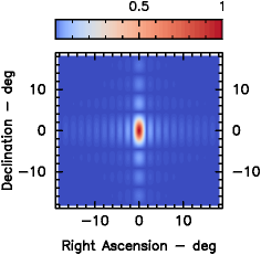
(a) $\delta_{0}=0^{\circ}$

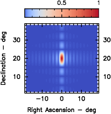
(b) $\delta_{0}=20^{\circ}$

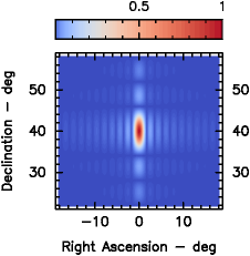
(c) $\delta_{0}=40^{\circ}$

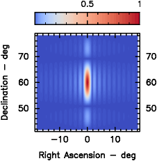
(d) $\delta_{0}=60^{\circ}$

Figure 6: The primary beam power pattern at declinations (a) $\delta_{0}=0^{\circ}$, (b) $20^{\circ}$, (c) $40^{\circ}$ and (d) $60^{\circ}$. The beam widens noticeably in declination extent at higher declination as the projected aperture size shrinks as $\cos\ \!\delta_{0}$.

4.4 Sky and model visibilities

The model visibilities are computed as described below. In the model for the foregrounds, only two components are considered here as they are the most dominant at 326.5 MHz. The diffuse Galactic synchrotron foreground dominates the emission from within the Galaxy at very large scales($\>2^{\circ}$), while the extragalactic sources dominate at scales typically smaller than a degree(Ali & Bharadwaj, 2014). Random realisations of the foreground emission are obtained from the assumed power spectrum of the emission: the details of how they are generated are explained in Marthi et al. (2017), however a very brief description follows.

For the Galactic diffuse foreground, a random realisation of the angular power spectrum is generated on a Fourier grid, the values of which are given by

$$\Delta\tilde{S}(u,\nu)=\left(\frac{\partial B}{\partial T}\right)\sqrt{\frac{\Omega\,C_{\ell}(\nu)}{2}}\left(x+iy\right)$$ (12)

where $\Delta\tilde{S}(u,\nu)$ represents the Fourier transform of the intensity fluctuations. $\Omega$ is the solid angle of the sky to be simulated, $C_{\ell}$ is the angular power spectrum, $x$ and $y$ are Gaussian random variables with zero mean and unit variance. An inverse Fourier transform of the populated Fourier grid now gives a single random realisation of the diffuse foreground.

The extragalactic foreground is similarly obtained from an angular power spectrum, but it is more involved than the simple Fourier inversion in the diffuse foreground case. We therefore follow the method of González-Nuevo, Toffolatti & Argüeso (2005) by modifying the Poisson density contrast field by the clustering power spectrum and populating the modified density field with sources drawn from the radio source counts at 325 MHz (Wieringa, 1991).

Once the maps are available, their individual components are superimposed in sky-coordinates to obtain the total emission from the sky.

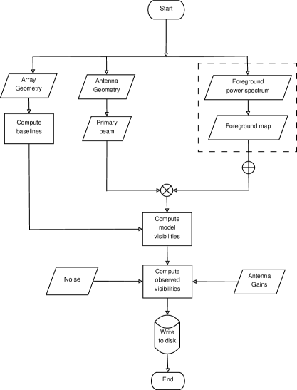
Figure 7: This flowchart gives an overall picture of the part of the simulator that produces the model and observed visibilities.

The specific intensity function is then given by

$$I(\alpha,\delta,\nu)=\Delta I_{D}(\alpha,\delta,\nu)\ +\ \sum\limits^{L}_{k=1}I_{k}(\alpha_{k},\delta_{k},\nu)$$ (13)

where $\Delta I_{D}(\alpha,\delta,\nu)$ is the fluctuation in the specific intensity of the diffuse foreground emission, and the $L$ distinct extragalactic radio sources are identified by their co-ordinates $(\alpha,\delta)$ and specific intensities $I_{k}$. The discrete sources are each confined to a pixel, so that the specific intensity of each source is equal to its flux density. For the diffuse foregrounds, the simulated maps are already pixelised, and the specific intensity in each pixel has already been scaled by the solid angle of the pixel. The flux density of the sky is

$$S(\alpha,\delta,\nu)=\Delta S_{D}(\alpha,\delta,\nu)+\ \sum\limits^{L}_{k=1}S_{k}(\alpha_{k},\delta_{k},\nu)$$ (14)

Since the model visibilities $M(\mathbf{U},\nu)$ for the non-redundant set of baselines are obtained as a pixel-by-pixel Fourier sum of the primary-beam weighted specific intensity distribution, we finally have

$$\mathbf{M}(\mathbf{U},\nu)=\sum\limits_{\alpha,\delta}\ S(\alpha,\delta,\nu)\ \mathbf{A}(\alpha,\delta,\nu)\ e^{-i2\pi\mathbf{U}.\mathbf{\hat{n}}}$$ (15)

which is the discretized version of equation 6.

The observing band is centered at 326.5 MHz with a bandwidth of $\sim 39$ MHz split into 312 channels in the simulations. The frequency resolution in this case is 125 kHz per channel. Based on our understanding of the distribution of the neutral gas around the redshift of $z\sim 3.35$, it is expected that the Hi signal at two redshifted frequencies, separated by more than $\Delta\nu$ of 1 MHz, decorrelates rapidly(see e.g. Bharadwaj & Ali, 2005). This means that with a channel resolution of 125 kHz, the Hi signal correlation is adequately sampled over the 1-MHz correlation interval. In reality, the channel resolution is likely to be much finer($\sim 50\mathrm{kHz}$), with about 800 channels across the $\sim$39-MHz band. This is useful for the identification and excision of narrow line radio frequency interference. Beyond the need to handle RFI, there is no real incentive to retain the visibility data at this resolution at the cost of downstream computing and storage requirements. Eventually, we may smooth the data to a resolution of 125 kHz, keeping in mind the decorrelation bandwidth of the Hi signal. The emulator itself is indeed capable of running at any frequency resolution, including the actual final configuration of the Phase-I and Phase-II systems. But the 125-kHz resolution used in the simulations allows for rapid processing, especially if they are to be run repetitively for a wide range of different parameters.

The model visibilities $\mathbf{M(U)}$ need be obtained only for the set of distinct non-redundant baselines, denoted by $\mathbf{U}_{|i-j|}$. The observed visibility $V_{ij}$ for a baseline with antennas $i$ and $j$ depends on the model visibility for that particular spacing $M(_{|i-j|})$, as well the gains of the individual antennas:

$$V_{ij}\left(U_{|i-j|}\right)=g_{i}\ g_{j}^{*}\ M\left(U_{|i-j|}\right)+N_{ij}\left(\nu\right)$$ (16)

where $M$ is the model visibility including the primary beam as described above, $g_{i}$ and $g_{j}$ are the complex antenna gains and $N_{ij}$ is the complex Gaussian random noise equivalent to the system temperature $T_{\mathrm{sys}}$. The real and imaginary parts of the noise $N_{ij}$ in equation 16 have a RMS fluctuation

$$\sigma_{ij}=\frac{\sqrt{2}k_{B}T_{\mathrm{sys}}}{\eta A\sqrt{\Delta\nu\Delta t}}$$ (17)

per channel, where $k_{B}$ is the Boltzmann constant, $\eta$ is the aperture efficiency, $A=b\times d$ is the aperture area, $\Delta\nu$ the channel width and $\Delta t$ the integration time. The foreground maps give the flux in Jy units at every pixel, therefore the Fourier sum directly produces the model visibilities in Jy units as well. The flowchart in Figure 7 gives a bird’s eye view of the part of the simulator pipeline used to obtain the visibilities, and summarises the emulator part of Prowess. The dashed box in the flowchart represents the functionality that simulates the foreground maps. The emulator also has the functionality to accept an external FITS image(e.g. via observations from some other telescope) of the foreground.

4.5 Redundancy calibration

Due to the highly redundant configuration of OWFA, the number of independent Fourier modes measured on the sky is small, given by a small number of baselines, $N_{A}-1$. All other baselines give copies of these measurements. As a result, we obtain a system of equations in which the number of unknowns is much smaller than the number of measurements. This allows us to not only solve for the gains of the antennas but, unlike routine interferometric calibration, also solve for the true sky visibilities. This class of calibration algorithms is called redundancy calibration(see Wieringa, 1992; Liu et al., 2010, for examples). Prowess implements a highly efficient, fast and statistically optimal non-linear least squares minimisation based steepest descent calibration, that is capable of running in real time. This calibration algorithm, detailed in Marthi & Chengalur (2014), is the algorithm of choice for OWFA. Denoting the antenna gains as $g_{i}$, the true visibilities as $M_{|i-j|}$ and the observed visibilities as $V_{ij}$, the gains and the true visibilities are solved for iteratively using the equations

$$g_{k}^{n+1}=(1-\alpha)g_{k}^{n}+\alpha\mathbf{Q_{k}}^{n}$$ (18)

and

$$M_{|k-j|}^{n+1}=(1-\alpha)M_{|k-j|}^{n}+\alpha\mathbf{R_{kj}}^{n}$$ (19)

where

$$\mathbf{Q_{k}}=\frac{\sum\limits_{j\neq k}w_{kj}g_{j}M_{|k-j|}^{*}V_{kj}}{\sum\limits_{j\neq k}w_{kj}|g_{j}|^{2}\ |M_{|k-j|}|^{2}},$$ (20)

$$\mathbf{R_{kj}}=\frac{\sum\limits_{j>k}g_{k}^{*}g_{j}V_{kj}}{\sum\limits_{j>k}w_{kj}|g_{k}|^{2}|g_{j}|^{2}}$$ (21)

and $0<\alpha<1$ is the step size. The gains and true visibilities at the present instant are obtained as updates to those obtained in the previous instant. The simulated visibilities are therefore calibrated using this algorithm to obtain the true visibilities. Redundancy calibration is a model-independent calibration procedure; hence the sky model is a natural product of calibration.

4.6 Power spectrum estimation

The calibrated visibility data are processed directly to obtain the power spectrum. A visibility-based angular power spectrum estimator has been implemented in Prowess. The estimator has been studied in earlier works(Begum, Chengalur & Bhardwaj, 2006; Datta, Choudhury & Bharadwaj, 2007; Choudhuri et al., 2014), but it has been recast for OWFA. Prowess implements the estimator to take advantage of the redundant baseline configuration of OWFA, allowing us to add the visibilities from all the redundant copies of a baseline of a given length. The implementation of the estimator is detailed in Marthi et al. (2017). Denoting the calibrated visibility as $\mathcal{V}(\mathbf{U}_{n},\nu)$, let us define the quantity

$$\mathcal{V}^{\prime}(\mathbf{U}_{n},\nu)=\sum_{i=0}^{N_{n}}|\mathcal{V}^{(i)}(\mathbf{U}_{n},\nu)|^{2}$$ (22)

We can now define our estimator, $\mathbf{S}_{2}$, as

$$\mathbf{S}_{2}(\mathbf{U}_{n},\nu_{i},\nu_{j})=\frac{\mathcal{V}(\mathbf{U}_{n},\nu_{i})\mathcal{V}^{*}(\mathbf{U}_{n},\nu_{j})-\delta_{ij}\mathcal{V}^{\prime}(\mathbf{U}_{n},\nu_{i})}{N_{n}^{2}-\delta_{ij}N_{n}}$$ (23)

The second term in the numerator corrects for the bias contributed by the self-correlated noise. For an N-channel visibility dataset, the real-valued $\mathbf{S}_{2}(\mathbf{U}_{n},\nu_{i},\nu_{j})$ is a $N\times N$ matrix as implemented in Prowess. This representation in the $\nu-\nu$ plane has its advantages in the study of systematics as it retains the full spectral information of the foregrounds and those introduced by the instrument. The estimator matrix cube is available in FITS format that can be visulaised either through standard FITS visualisation programs or through the tool implemented in Prowess.

The study of foreground power spectra through simulations, enabled by Prowess, inform us that per-baseline spectral features arising in the estimator within the observing band are caused by (i) the effect of the frequency-dependent primary beam and (ii) the frequency dependence of the baseline vector. These effects have been studied in some detail in the context of EoR experiments, such as by Vedantham, Udaya Shankar & Subrahmanyan (2012) for example. We have carried out exhaustive studies of instrumental chromatic effects on the power spectrum for OWFA (Marthi et al., 2017). Importantly, simulations using Prowess appear to indicate that the instrinsic chromatic properties of the sky are less important, but such chromatic effects are compounded by the chromatic instrument response. These effects would eventually play a limiting role in the detectability of the Hi signal.

4.7 Data visualisation

The simulated visibilities are written into a FITS file in the UVFITS data format. This is a standard format for reading and writing the radio interferometric visibility data, and is the format being used at the GMRT. However, Prowess has its own interface that helps in visualising the visibility data, which is explained here. The data are available in time-baseline-frequency order. That is, the coarsest data identifier is the record number, which is tagged to the timestamp. At each timestamp, all the ${}^{N_{A}}C_{2}$ baselines are sorted in a specific order, indexed by the FITSbl

Figure 8: The display buffer with gridded Time, Frequency and Baseline axes, where the complex visibility resides.

number shown in Figure 4. Each baseline has $N$ channels, and each channel has a real and imaginary number for the visibility, and an associated weight. The visibility data therefore reside in a

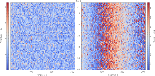
Figure 9: A time-frequency view of the visibility data on the $T-N$ plane for $B=1$.

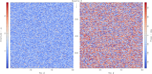
Figure 10: A time-baseline view of the visibility data on the $T-B$ plane for $N=156$.

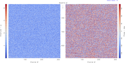
Figure 11: A frequency-baseline view of the visibility data on the $N-B$ plane for $T=30$.

gridded three-dimensional co-ordinate system where the three axes are time, baseline and frequency. There are $T\times B\times N$ grid cells, where $T$ is the number of records, $B$ is the number of baselines and $N$ is the number of channels, shown in Figure 8. This arrangement is very convenient; therefore the native structure that holds these visibility data in a display buffer is similarly defined. For visualising the data, they are therefore read from the FITS record into the display buffer. The visualisation programs hence access one of the planes parallel to the $T-B$, $B-N$ or $T-N$ planes. Figures 9,  10 and  11 show the simulated visibility accessed from the display buffer for an example run with a particular realisation for the diffuse Galactic foreground, with the 312-channel, 40-antenna, 780-baseline Phase-I observed for 60 seconds with a record being written to disk every second. There is an option to dynamically switch between a real/imaginary or an amplitude/phase view, and dynamically switch between linear, square-root and logarithmic image transfer functions. A dynamic zooming feature is available in these interfaces as well. Besides the colour-coded plan view, these plane data from the display buffer can also be viewed in a line-plot format, again, with the option to dynamically switch between real/imaginary and amplitude/phase view formats.

5 The observatory data processing pipeline

Prowess is not an emulator alone, as the name may suggest. It was described in Section 2 why the emulator was conceived: it serves the dual purpose of an emulator and would potentially become the standard post-correlation data processing pipeline at the observatory. It would be useful now to dwell a little on the data processing pipeline aspect of Prowess and state what functionality it is meant to provide.

The data pooled from the antennas would terminate in the eight high-performance compute nodes through eleven copper ethernet links each. These nodes correlate the signal from every pair of antennas and accumulate the products upto an interval of time, usually programmable. The typical integration time, called the Long Term Accumulation(LTA), is of the order of $1-10$ seconds. Once the data are available in FITS format, Prowess can completely take over downstream processing, which include calibration and power spectrum estimation. The uncalibrated FITS data can as well be stored in the disks for offline calibration. The enormous redundancy of the measurements and the structure of OWFA are best exploited by calibrating the visibilities using the non-linear least squares redundancy calibration algorithm, described in Section 4.5. The calibrated visibilities are later processed to obtain the power spectrum of observed sky.

6 Summary

A software model that captures the instrumental and geometric details of OWFA has been described. This detailed model is an important aid to understanding the systematics introduced by the instrument and to make robust and meaningful predictions for the foregrounds and the Hi signal. The programming philosophy allows for modular function definitions and easy addition of new functionality. The suite features a rich and interactive visual environment to play back the visibility data. These programs comprise not just an emulator for OWFA, but they are also designed to serve as observatory data analysis software. Prowess has greatly aided our understanding of the instrument and the systematics expected in the OWFA cosmology experiment.

References

- Ali & Bharadwaj (2014) Ali S. S., Bharadwaj S., 2014, JApA, 35, 157
- Ali, Bharadwaj & Chengalur (2008) Ali S. S., Bharadwaj S., Chengalur J. N., 2008, MNRAS, 385, 2166
- Bandura et al. (2014) Bandura K. et al., 2014, in Proc. SPIE, Vol. 9145, Ground-based and Airborne Telescopes V, p. 914522
- Begum, Chengalur & Bhardwaj (2006) Begum A., Chengalur J. N., Bhardwaj S., 2006, MNRAS, 372, L33
- Bharadwaj & Ali (2005) Bharadwaj S., Ali S. S., 2005, MNRAS, 356, 1519
- Bharadwaj, Sarkar & Ali (2015) Bharadwaj S., Sarkar A. K., Ali S. S., 2015, JApA, 36, 385
- Chen (2011) Chen X., 2011, Scientia Sinica Physica, Mechanica Astronomica, 41, 1358
- Choudhuri et al. (2014) Choudhuri S., Bharadwaj S., Ghosh A., Ali S. S., 2014, MNRAS, 445, 4351
- Datta, Choudhury & Bharadwaj (2007) Datta K. K., Choudhury T. R., Bharadwaj S., 2007, MNRAS, 378, 119
- González-Nuevo, Toffolatti & Argüeso (2005) González-Nuevo J., Toffolatti L., Argüeso F., 2005, Ap.J, 621, 1
- Iacobelli et al. (2014) Iacobelli M. et al., 2014, A & A, 566, A5
- Iacobelli, Haverkorn & Katgert (2013) Iacobelli M., Haverkorn M., Katgert P., 2013, A & A, 549, A56
- Iacobelli et al. (2013) Iacobelli M. et al., 2013, A & A, 558, A72
- Kemball & Wieringa (2000) Kemball A. J., Wieringa M. H., 2000, https://casacore.github.io/casacore-notes/229.html
- Liu et al. (2010) Liu A., Tegmark M., Morrison S., Lutomirski A., Zaldarriaga M., 2010, MNRAS, 408, 1029
- Marthi et al. (2017) Marthi V. R., Chatterjee S., Chengalur J., Bharadwaj S., 2017, MNRAS, under review
- Marthi & Chengalur (2014) Marthi V. R., Chengalur J., 2014, MNRAS, 437, 524
- Pober et al. (2013) Pober J. C. et al., 2013, AJ, 145, 65
- Prasad & Subrahmanya (2011) Prasad P., Subrahmanya C. R., 2011, Exp. Astron., 31, 1
- Price, Barsdell & Greenhill (2015) Price D. C., Barsdell B. R., Greenhill L. J., 2015, in Astronomical Society of the Pacific Conference Series, Vol. 495, Astronomical Data Analysis Software an Systems XXIV (ADASS XXIV), Taylor A. R., Rosolowsky E., eds., p. 531
- Santos, Cooray & Knox (2005) Santos M. G., Cooray A., Knox L., 2005, Ap.J, 625, 575
- Sarkar, Bharadwaj & Ali (2017) Sarkar A. K., Bharadwaj S., Ali S. S., 2017, JApA, special issue on OWFA
- Subrahmanya, Manoharan & Chengalur (2017) Subrahmanya C. R., Manoharan P. K., Chengalur J. N., 2017, JApA, special issue on OWFA
- Subrahmanya et al. (2017) Subrahmanya C. R., Prasad P., Girish B. S., Somasekhar R., Manoharan P. K., Amit Mittal S. G., 2017, JApA, special issue on OWFA
- Swarup et al. (1971) Swarup G. et al., 1971, Nature Physical Science, 230, 185
- Vedantham, Udaya Shankar & Subrahmanyan (2012) Vedantham H., Udaya Shankar N., Subrahmanyan R., 2012, Ap.J, 745, 176
- Wells, Greisen & Harten (1981) Wells D. C., Greisen E. W., Harten R. H., 1981, A & AS, 44, 363
- Wieringa (1991) Wieringa M. H., 1991, PhD thesis, Rijksuniversiteit Leiden, (1991)
- Wieringa (1992) Wieringa M. H., 1992, Experimental Astronomy, 2, 203
- Xu, Wang & Chen (2015) Xu Y., Wang X., Chen X., 2015, Ap.J, 798, 40