Fundamental Vortices, Wall-Crossing, and Particle-Vortex Duality

Abstract

We explore 1d vortex dynamics of 3d supersymmetric Yang-Mills theories, as inferred from factorization of exact partition functions. Under Seiberg-like dualities, the 3d partition function must remain invariant, yet it is not a priori clear what should happen to the vortex dynamics. We observe that the 1d quivers for the vortices remain the same, and the net effect of the 3d duality map manifests as 1d Wall-Crossing phenomenon; Although the vortex number can shift along such duality maps, the ranks of the 1d quiver theory are unaffected, leading to a notion of fundamental vortices as basic building blocks for topological sectors. For Aharony-type duality, in particular, where one must supply extra chiral fields to couple with monopole operators on the dual side, 1d wall-crossings of an infinite number of vortex quiver theories are neatly and collectively encoded by 3d determinant of such extra chiral fields. As such, 1d wall-crossing of the vortex theory encodes the particle-vortex duality embedded in the 3d Seiberg-like duality. For $\mathcal{N}=4$, the D-brane picture is used to motivate this 3d/1d connection, while, for $\mathcal{N}=2$, this 3d/1d connection is used to fine-tune otherwise ambiguous vortex dynamics. We also prove some identities of 3d supersymmetric partition functions for the Aharony duality using this vortex wall-crossing interpretation.

1 Introduction

In recent years, a plethora of exact partition functions became available for supersymmetric gauge theories. The localization method, responsible for these, is powerful and universal but such universality comes with costs. Much of the dynamics is lost, as the end result depends only on handful of UV information, such as field contents and their representation under the gauge and the global symmetries. This should be hardly surprising. When the spacetime that admits a circle, for example, the supersymmetric partition function can be regarded as a refined index, well-known to be robust under continuous deformations. Despite this ultraviolet nature of the computation, these partition functions proved to quite useful, for example as a litmus test for various dualities. For dimensions less than three also, where there is no notion of vacuum expectation value of moduli, a UV theory often flows down to a unique theory in IR. As such, the partition functions in such low dimensions contain more useful information than one may generally hope for. The Gromov-Witten invariants cleverly embedded Jockers:2012dk ; Gomis:2012wy in the $S^{2}$ partition functions Benini:2012ui ; Doroud:2012xw of $d=2$ GLSM are the prime example of this, while the $d=2$ elliptic genus Benini:2013xpa and $d=1$ refined Witten index Hori:2014tda are more obvious ones.

A trick of convenience involved in the localization computations, which lifts flat directions as much as possible, is to introduce chemical potentials and other susy-preserving masses. For $d=3$ theories, in particular, one turns on real masses associated with flavor symmetries, which generically simplify the vacuum structures to those of isolated ones. Note that not all theories admit such computations. When the theory must involve superpotentials, for example, the number of the available flavor symmetries get reduced. Also, given a reduced flavor symmetry that allows some superpotential, the computation will tend to compute the partition function for theories with generic superpotential consistent with the flavor charge assignment. The usual mantra that the localization is insensitive to the details of the superpotential must be taken with such genericity presumed. In this note, we will be considering theories where all matter fields acquire real masses, independent of one another, which means that superpotential is turned off by imposing global symmetries.

When the number of matter multiplets and accompanying flavor symmetry are sufficiently large, quantum vacua then tend to be isolated Intriligator:2013lca . One type, which we refer to as the Higgs vacua, is such that chiral fields are turned on to cancel FI constants with the Coulombic vev’s pinned at some of the real masses. Another type, more characteristic of $d=3$ and called the topological vacua by Intriligator and Seiberg, achieves the vacuum condition entirely along the Coulomb branch with all chiral fields turned off. Although the total number of vacua is invariant under continuous deformations of the theory, this split of vacua between the Higgs type and the topological type is not robust, and in particular affected by signs of 3d FI constants. One interesting class of theories is where one can tune the 3d FI constant so that all vacua are of Higgs variety. In such theories, the exact partition functions on $S^{1}$ fibred over $S^{2}$ are known to admit the so-called factorization Krattenthaler:2011da ; Dimofte:2011ju ; Pasquetti:2011fj ; Beem:2012mb ; Hwang:2012jh ; Taki:2013opa ; Cecotti:2013mba ; Fujitsuka:2013fga ; Benini:2013yva ; Benini:2015noa where the partition function can be rewritten as a sum over product of three multiplicative pieces: vortex contributions at the north pole, anti-vortex contributions at the south pole, and the perturbative 1-loop from fields not involved in the vortex construction.

When a partition function is thus factorizable, one has a good glimpse into the supersymmetric vortices. In an isolated Higgs vacuum, one chiral field gets a vev on top of each Cartan vev $\sigma_{a}$ pinned at a real mass $m_{i}$, and form ${\mathbb{P}}^{0}$ after the gauge identification. Each such chiral field can acquire the winding number and the associated quantized magnetic flux $2\pi n_{a}$. Due to the chemical potential associated with $R+2J_{3}$ where $R$ is an R-symmetry generator and $J_{3}$ a rotation generator on $S^{2}$, the (anti-)vortices are pushed into the north(south)-pole, much like the $\Omega$-deformation on ${\mathbb{R}}^{4}$ pushing instantons to the origin Nekrasov:2002qd .

As such, contributions of vortices and of anti-vortices to the partition function can be read off from the factorization, and in turn one can ask what low energy dynamics of vortices is capable of producing such contributions. This gives us an indirect way to explore $d=1$ low energy dynamics of vortices, from 3d exact partition functions. The latter is reliably and universally computed via the Coulombic localization, which has no knowledge of the Higgs vacua or of vortices. Yet, it can be used to extract vortex dynamics, once factorized.

The vortex theory found this way is typically a quiver quantum mechanics with either ${\cal N}=4$ or ${\cal N}=2$ supercharges, respectively, for 3d ${\cal N}=4$ or ${\cal N}=2$ gauge theories. Since the partition function itself carries limited information about the 3d field theory, one should not really expect the exact low energy dynamics of the vortices Hanany:2003hp ; Rather, we are interested in more robust (hence more coarse) aspects of the low energy dynamics, as much as can be encoded in the 1d twisted partition functions of vortices. The main question we ask is how the 3d Seiberg-like dualities manifest in the 1d vortex theory, and what else we learn from such investigations.

Since Seiberg-like dualities change the UV data of 3d theory entirely, it is not clear whether there is a simple meaningful action of this duality on vortices themselves. It does preserve the partition function, yet we are asking about individual vortex sector contributions, an infinite number of which must be combined to contribute to a single 3d partition function. Also the rank of the 3d theory changes and vortices are naturally associated with the Cartan part of the gauge group, so the vortex number must change upon duality, even if somehow the contributions remain intact sector by sector. This seems a contradiction in itself, as we usually interpret the vortex contribution as coming from the low energy quantum mechanics of the relevant topological sector, which is in turn closely related to the Cartan $U(1)$’s of the gauge group.

A useful analogy can be learned from BPS monopoles in $d=4$ Weinberg:1982ev ; Weinberg:2006rq . For a non-Abelian Yang-Mills broken to the Cartan by a single adjoint Higgs field, there can be as many “unit” magnetic monopole solutions as the number of positive roots; Along each positive root, one can embed $SU(2)$ and a unit magnetic monopole solution thereof. Upon a closer look, however, one quickly realizes that most of such monopoles are composite states of more than one “fundamental” monopoles Weinberg:1982ev . Recall that the fundamental monopole makes sense when the Yang-Mills group is broken to the Cartan, with help of real adjoint Higgs vev $h$. The latter defines the positivity in the dual root space, which in turn divides monopoles into BPS and anti-BPS. A BPS monopole, associated with positive dual root $\alpha^{*}$, is then generally written as

$$\alpha^{*}=\sum n_{a}\beta^{*}_{a}$$

with nonnegative integers $n_{a}$, which defines the fundamental monopole charges $\beta^{*}_{a}$. It is easy to see that the collection $\{\beta_{a}\}$ can be regarded as a collection of simple roots, with the positivity defined by $h$, and mass of the monopole is built additively from masses of these fundamental monopoles. Such a monopole is separable into $\sum_{a}n_{a}$ distinct fundamental monopoles in real space.

Similarly, we will find that a notion of “fundamental” vortices emerges quite naturally. For vortices in $\mathcal{N}=2$ theories, the 3d FI constants $\xi$, regarded as a vector in the gauged Cartan subalgebra, will play the analog of $h$ while the roles of magnetic charges (such as $\alpha^{*}$ and $\beta_{a}^{*}$) are played by the Chern numbers $q$ of the vortices. As with the monopole analogy, the fundamental vortices are those with “minimal” positive masses $\xi\cdot q_{i}>0$, so that general positive vortices are constructed as

$$q=\sum k_{i}q_{i}$$

with nonnegative integer $k_{i}$’s. For 3d $\mathcal{N}=4$ theories, for which $\xi$’s are naturally triplets, we must also address why it makes sense to pick out one out of three possible directions for $\xi$, which will be addressed later.

Then, what does happen to the theory of such fundamental vortices when 3d duality is performed? Much like ADHM of instantons, the effective quantum mechanics of vortices, whenever known, is of quiver type. Although this representation is not accurate enough in dynamical sense, it appears to be good enough for some supersymmetric observables such as the twisted partition function that enters the 3d partition functions. Our finding shows the following: the quiver theory for vortices remains invariant, quite surprisingly, upon Seiberg-like duality. Not only the quiver itself is invariant, so are the rank vectors. Clearly, this 1d quiver theory describes the dynamics of the fundamental vortices, and the invariance implies that the notion of these fundamental vortices is also robust under the 3d duality as long as we correctly keep track of signs of 3d FI constants along the Seiberg-like duality. The rule for the latter can be naturally inferred from quiver mutation mechanism along with their underlying D-brane pictures.

Instead, the 1d vortex theory reacts to 3d duality by flipping sign(s) of some 1d FI parameters $\zeta$. Recall that in supersymmetric gauged quantum mechanics, the sign flip of an FI parameter often causes a wall-crossing Denef:2002ru . At the level of computation via JK-residue sum, the sign flip implies that the list of contributing residues changes. Depending on details of the quiver theory, this may or may not translate to different twisted partition functions in the end Hori:2014tda . When the result remains unchanged after the residue sum, our assertion implies that not only the vortex quiver theory but the twisted partition function contributing to 3d partition functions remain exactly the same despite the Seiberg-duality. Since the vortex numbers in 3d sense differ between dual pairs, we will also identify a canonical 3d theory in a given duality chain where the fundamental vortices are identified by “unit” Chern numbers and where the resulting vortex quiver theory is most naturally identified.

When 1d twisted partition functions do change, signalling nontrivial wall-crossing in the vortex quiver theory, a new issue arises. Since such a wall-crossing tends to be universal for all rank vectors, the discrepancies exist in an infinite number of vortex sectors. On the other hand, 3d partition function itself has to be invariant under the duality, so there has to be something else that corrects this change of vortex contributions. The answer to this is also simple and elegant: Such discrepancies exist if and only if the Seiberg-like duality becomes an Aharony type Aharony:1997gp , where one must insert extra neutral chiral multiplets on the dual side, usually coupled to monopole operators via F-term. Furthermore, an infinite number of discrepancies sum up exactly to the simple perturbative contributions from such extra chiral multiplets on the dual side, compensating the difference neatly. In effect, whenever the 1d vortex theory undergoes a wall-crossing, we are witnessing a particle-vortex duality embedded in the 3d Seiberg-like duality.

On the other hand, we must caution the readers against taking the low energy theory of vortices too literally. What they keep track of is topological information rather than dynamical one. For instance there are cases where, even though the vortex quiver theory looks nontrivial, it has no supersymmetric vacua and thus offers no accompanying vortex contribution to the 3d partition function. This commonly indicates that the vortex in question cannot be quantized preserving supersymmetry, but could also happen simply because one side of a 3d dual pair has no gauge group. Clearly, we cannot really speak of vortex dynamics in any dynamical sense on the side with no 3d gauge group, yet, amazingly, the common 1d vortex quiver theory, naturally derived on the gauged side, correctly keeps track of “vortex” contributions to both sides. In the absence of 1d wall-crossing, this would tell us the gauged side has no supersymmetric and quantum vortex even though such a solution is possible classically; in the presence of 1d wall-crossing, this would indicate that a complete vortex-particle duality has occurred. In a way, such versatility of these 1d fundamental vortices is both puzzling and intriguing.

In this note, we study and explore such relations between 3d Seiberg-like dualities and 1d wall-crossings with emphasis on concrete examples. For $d=3$ ${\cal N}=4$ theories, the 3d/1d relation can be recovered quite straightforwardly from Hanany-Witten D-brane realizations which also tell us much about the 1d quiver theory of vortices. For 3d ${\cal N}=2$ theories, things are no longer so simple. Among various complications are the rampant Chern-Simons terms and how they modify the 1d quiver theory. Although the general answer to this can be seen to be supersymmetry-preserving Wilson lines in the vortex quantum mechanics, we find the details of how this is realized are actually ambiguous if one cares only about the final twisted partition functions, chamber by chamber. In contrast, our main observation, which gives an unambiguous rule for connecting different 1d chambers and thus related 3d Seiberg-dual theories, will be used to resolve such ambiguities.

In section 2, we review some background materials for 3d supersymmetric gauge theories and 1d gauged linear sigma model. In section 3, we discuss the quantum mechanics descriptions for half-BPS vortices in 3d $\mathcal{N}=4,2$ linear quiver gauge theories and compute their refined Witten indices. In section 4, we examine the connection between vortex quantum mechanics and 3d Seiberg-like dualities, in particular, for $\mathcal{N}=2,4$ SQCD-like theories with (anti-)fundamental matters and linear quiver theories with bi-fundamental matters. Section 5 is a summary of the note. We also work out the factorization of the topologically twisted index on $S^{2}\times S^{1}$ in Appendix A and prove some identities of 3d supersymmetric partition functions for the Aharony duality in Appendix B.

2 Review

2.1 3d $\mathcal{N}=2$ gauge theories and Seiberg-like dualities

In this section we review some basic properties of 3d $\mathcal{N}=2$ supersymmetric gauge theories, which will be relevant in the subsequent sections. As a concrete example, we consider a 3d $\mathcal{N}=2$ theory with gauge group $U(N_{c})$. The theory contains an $\mathcal{N}=2$ vector multiplet, which consists of a gauge field $A$, a real scalar $\sigma$, a two-component Dirac fermion, called a gaugino, $\lambda$ and an auxiliary real scalar $D$ in the adjoint representation of the gauge group $U(N_{c})$. One can also introduce a chiral multiplet, which consists of a complex scalar $\phi$, a two-component Dirac fermion $\psi$ and an auxiliary complex scalar $F$. We here consider $N_{f}$ chiral multiplets $Q_{a}^{i}$ in the fundamental representation and $N_{a}$ chiral multiplets $\tilde{Q}_{i}^{\tilde{b}}$ in the anti-fundamental representation where $a=1,\ldots,N_{f}$, $\tilde{b}=1,\ldots,N_{a}$ and $i=1,\ldots,N_{c}$. A holomorphic function $W(Q,\tilde{Q})$ of those chiral multiplets defines the superpotential, which yields interaction terms of the theory.

Another type of an interaction that a 3d $\mathcal{N}=2$ theory has is the Chern-Simons interaction. For the gauge group $U(N_{c})$, one can include the CS interaction of level $\kappa$:

$$\mathcal{L}_{\text{CS}}^{\mathcal{N}=2}=\frac{\kappa}{4\pi}\mathrm{Tr}\left(\epsilon^{\mu\nu\rho}\left(A_{\mu}\partial_{\nu}A_{\rho}-\frac{2i}{3}A_{\mu}A_{\nu}A_{\rho}\right)+2D\sigma+\overline{\lambda}\lambda\right)$$ (1)

where $\kappa$ should satisfy $\kappa+\frac{N_{f}-N_{a}}{2}\in\mathbb{Z}$ due to the so-called parity anomaly. Moreover, one can also turn on the additional CS interaction for the $U(1)$ factor of the gauge group. This $U(1)$ CS interaction can be generalized such that one can consider a CS-like interaction between different $U(1)$ symmetries:

$$\mathcal{L}_{\text{BF}}^{\mathcal{N}=2}=\frac{1}{2\pi}\left(\epsilon^{\mu\nu\rho}A^{(1)}_{\mu}\partial_{\nu}A^{(2)}_{\rho}+D^{(1)}\sigma^{(2)}+D^{(2)}\sigma^{(1)}+\frac{1}{2}\left(\overline{\lambda}^{(1)}\lambda^{(2)}+\overline{\lambda}^{(2)}\lambda^{(1)}\right)\right).$$ (2)

This is called a mixed CS interaction, or a BF interaction because it is a coupling between field strength $F$ of gauge field $A^{(1)}$ and another gauge field $B=A^{(2)}$. In particular there is a special kind of a BF interaction which corresponds to the Fayet-Iliopoulos term. In 3d, a $U(N_{c})$ gauge theory has a global symmetry whose conserved current is defined as follow:

$$j=\frac{1}{2\pi}*\mathrm{Tr}F.$$ (3)

This is usually called the topological symmetry, which we will denote by $U(1)_{T}$. If we consider the BF interaction between this $U(1)_{T}$ global symmetry and the $U(1)$ factor of the gauge symmetry, it gives rise to the following Lagrangian, which is the same as the FI term:

$$\mathcal{L}_{\text{FI}}^{\mathcal{N}=2}=\frac{1}{2\pi}D\xi$$ (4)

where $\xi$ is the real scalar in the background vector multiplet for the $U(1)_{T}$ symmetry.

The theory has the $U(1)_{R}$ R-symmetry as well as other global symmetries $SU(N_{f})\times SU(N_{a})\times U(1)_{A}\times U(1)_{T}$. The charges of the fundamental and anti-fundamental chiral multiplets $Q,\tilde{Q}$ are summarized in table 1.

	$U(N_{c})$	$SU(N_{f})$	$SU(N_{a})$	$U(1)_{A}$	$U(1)_{T}$	$U(1)_{R}$
$Q$	$\mathbf{N_{c}}$	$\mathbf{\overline{N_{f}}}$	$\mathbf{1}$	$1$	$0$	$0$
$\tilde{Q}$	$\mathbf{\overline{N_{c}}}$	$\mathbf{1}$	$\mathbf{N_{a}}$	$1$	$0$	$0$
$q$	$\mathbf{N_{c}}$	$\mathbf{1}$	$\mathbf{\overline{N_{a}}}$	$-1$	$0$	$1$
$\tilde{q}$	$\mathbf{\overline{N_{c}}}$	$\mathbf{N_{f}}$	$\mathbf{1}$	$-1$	$0$	$1$
$M$	$\mathbf{1}$	$\mathbf{\overline{N_{f}}}$	$\mathbf{N_{a}}$	$2$	$0$	$0$
$V_{\pm}$	$\mathbf{1}$	$\mathbf{1}$	$\mathbf{1}$	$-\frac{N_{f}+N_{a}}{2}$	$\pm 1$	$\frac{N_{f}+N_{a}}{2}-N_{c}+1$

Table 1: The symmetry charges of the chiral multiplets we introduce. Note that $V_{\pm}$ exist only when $\kappa\pm\frac{N_{f}-N_{a}}{2}=0$ respectively. The $U(1)_{R}$ charges are UV values we conventionally choose. Their IR superconformal values are given by combinations of the UV R-charge and other global $U(1)$ charges, which can be determined by $Z$-extremization Jafferis:2010un .

Without the superpotential, the theory has supersymmetric vacua when $\textrm{max}\left(\kappa,\frac{|N_{f}-N_{a}|}{2}\right)+\frac{N_{f}+N_{a}}{2}\geq N_{c}$. The analysis of those supersymmetric vacua can be found in, e.g., Aharony:1997bx ; Giveon:2008zn ; Intriligator:2013lca . Here we briefly summarize the analysis of Intriligator:2013lca for a $U(1)$ theory.

After integrating out the auxiliary fields, one has the following semi-classical effective potential:

$$V=\frac{e_{\text{eff}}^{2}}{32\pi^{2}}\left(\sum_{i}2\pi n_{i}|Q_{i}|^{2}-\xi_{\text{eff}}-\kappa_{\text{eff}}\sigma\right)^{2}+\sum_{i}(m_{i}+n_{i}\sigma)^{2}|Q_{i}|^{2}$$ (5)

where $Q_{i}$ is the scalar in the $i$-th chiral multiplet of charge $n_{i}$ and real mass $m_{i}$. $e_{\text{eff}}$ is the effective gauge coupling. The quantum corrected FI parameter and CS level, $\xi_{\text{eff}}$ and $\kappa_{\text{eff}}$, are given by

$$\xi_{\text{eff}} =\xi+\frac{1}{2}\sum_{i}n_{i}m_{i}~{}\textrm{sgn}(m_{i}+n_{i}\sigma),$$ (6)

$$\kappa_{\text{eff}} =\kappa+\frac{1}{2}\sum_{i}n_{i}^{2}~{}\textrm{sgn}(m_{i}+n_{i}\sigma).$$ (7)

The semi-classical vacua are given by the solutions of $V=0$, or equivalently

$$F(\sigma)=\sum_{i}2\pi n_{i}|Q_{i}|^{2},$$ (8)

$$(m_{i}+n_{i}\sigma)Q_{i}=0$$ (9)

where we have defined

$$F(\sigma) \equiv\xi_{\text{eff}}+\kappa_{\text{eff}}\sigma$$ (10)

$$=\xi+\kappa\sigma+\frac{1}{2}\sum_{i}n_{i}|m_{i}+n_{i}\sigma|.$$ (11)

Equations (8) and (9) allow three types of solutions: Higgs, Coulomb and topological vacua. A Higgs vacuum is a solution with the nonzero vacuum expectation value $\left<Q_{i}\right>$. Nonzero $\left<Q_{i}\right>$, from (9), requires the vanishing effective real mass, $m_{i}+n_{i}\sigma=0$. For generic real masses, the Higgs vacua are isolated while for special values of real masses, they can have a continuous moduli space called a Higgs branch.

A Coulomb vacuum is a solution with $\xi_{\text{eff}}=\kappa_{\text{eff}}=0$, which implies that $F(\sigma)=\sum_{i}2\pi n_{i}|Q_{i}|^{2}=0$. There is a continuous moduli space of Coulomb vacua, which is parameterized by $\sigma$ in a range keeping $\xi_{\text{eff}}=\kappa_{\text{eff}}=0$. This is called a Coulomb branch.

A topological vacuum is a solution with $F(\sigma)=\sum_{i}2\pi n_{i}|Q_{i}|^{2}=0$ but with nonzero $\xi_{\text{eff}}$ and $\kappa_{\text{eff}}$. Unlike the Coulomb vacuum, a topological vacuum is isolated, which reflects the fact that there is no massless degree of freedom at a topological vacuum. Indeed, the low-energy effective theory at a topological vacuum is the $\mathcal{N}=2$ CS theory of level $\kappa_{\text{eff}}$. A classical topological vacuum obtained from $F(\sigma)=0$ acquires the topological multiplicity $|\kappa_{\text{eff}}|$ Witten:1999ds ; Intriligator:2013lca .

A 3d $\mathcal{N}=2$ $U(N_{c})$ theory is known to have a dual gauge description. More precisely, the 3d $\mathcal{N}=2$ $U(N_{c})_{\kappa}$ gauge theory with $N_{f}$ fundamental and $N_{a}$ anti-fundamental chiral multiplets flows to the same IR fixed point as the $U(N_{c}^{D})_{-\kappa}$ theory with $N_{a}$ fundamental and $N_{f}$ anti-fundamental chiral multiplets (and additional gauge singlet chiral multiplets we explain shortly) flows to. The dual gauge rank, $N_{c}^{D}$, is determined as follows:

$$N_{c}^{D}=\left\{\begin{array}[]{cc}\mathrm{max}(N_{f},N_{a})-N_{c},&|\kappa|\leq\frac{|N_{f}-N_{a}|}{2},\\ |\kappa|+\frac{N_{f}+N_{a}}{2}-N_{c},&|\kappa|>\frac{|N_{f}-N_{a}|}{2}.\\ \end{array}\right.$$ (14)

Originally the duality is proposed by Aharony for $\kappa=N_{f}-N_{a}=0$ Aharony:1997gp and by Giveon and Kutasov for $\kappa\neq N_{f}-N_{a}=0$ Giveon:2008zn . Later those are generalized to arbitrary $N_{f}$, $N_{a}$ and $\kappa$ Benini:2011mf .

The dual theory contains additional gauge singlet chiral multiplets which couple to the gauge theory via the superpotential. There are $N_{f}N_{a}$ chiral multiplets $M_{a}^{\tilde{b}}$ coupling to the dual fundamental and anti-fundamental chiral multiplets as follows:

$$W=M_{a}^{\tilde{b}}\tilde{q}^{i}_{\tilde{b}}q^{a}_{i}.$$ (15)

Those $M_{a}^{\tilde{b}}$ correspond to the meson operators in the original theory, $Q_{a}^{i}\tilde{Q}_{i}^{\tilde{b}}$, whose vacuum expectation values parameterize the Higgs branch of the moduli space. Due to the superpotential, the dual mesons $q^{a}_{i}q^{i}_{\tilde{b}}$ cannot have the vacuum expectation values.

In addition, there is another chiral multiplet $V_{\pm}$ if $\kappa=\mp\frac{N_{f}-N_{a}}{2}$ respectively. For each case, the dual theory has a gauge invariant monopole operator $v_{\mp}$, which couples to $V_{\pm}$ as follows:

$$W=\delta_{2\kappa,N_{a}-N_{f}}V_{+}v_{-}+\delta_{2\kappa,N_{f}-N_{a}}V_{-}v_{+}.$$ (16)

Due to this superpotential, $v_{\pm}$ cannot have the vacuum expectation values while the vacuum expectation values of $V_{\pm}$ parameterize the Coulomb branches of the moduli space. The charges of those extra chiral multiplets are summarized in table 1.

Note that the duality patterns for $N_{f}\neq N_{a}$ are distinguished into two classes: $|\kappa|<\frac{|N_{f}-N_{a}|}{2}$ and $|\kappa|>\frac{|N_{f}-N_{a}|}{2}$. In Benini:2011mf the former is called maximally chiral, whose duality pattern resembles the Aharony duality, while the latter is called minimally chiral, whose duality pattern resembles the Giveon-Kutasov duality. In this note, for brevity, we call the Seiberg-like dualities for $|\kappa|\leq\frac{|N_{f}-N_{a}|}{2}$ Aharony dualities and the dualities for $|\kappa|>\frac{|N_{f}-N_{a}|}{2}$ Giveon-Kutasov dualities.

The Aharony duality and the Giveon-Kutasov duality are inferred from the Hanany-Witten transitions Hanany:1996ie between the brane setups illustrated in figure 1 and figure 2.

Figure 1: The brane motion representing the Aharony duality. The spacetime directions occupied by each brane are summarized in table 2. Due to the Hanany-Witten effect, the number of the D3-branes changes from $N_{c}$ to $N_{f}-N_{c}$ when the NS5-brane passes through D5-branes.

Figure 2: The brane motion representing the Giveon-Kutasov duality. The spacetime directions occupied by each brane are summarized in table 2. For positive FI parameter $\xi>0$, one end of a D3-brane is attached either to D5-brane or to $(1,k_{+})$-brane. In the figure, $N^{\prime}$ D3-branes are ending on the $(1,k_{+})$-brane. Recall that $k_{+}=\kappa+\frac{N_{f}-N_{a}}{2}$, which is negative in the figure. After the NS5-brane passes through D5-branes, (and the $(1,k_{+})$-brane,) there are $|k_{+}|+N_{f}-N_{c}=|\kappa|+\frac{N_{f}+N_{a}}{2}-N_{c}$ D3-branes due to the Hanany-Witten effect.

Branes	0	1	2	3	4	5	6	7	8	9
NS5	$\times$	$\times$	$\times$	$\times$	$\times$	$\times$
$(1,k_{\pm})$	$\times$	$\times$	$\times$			$\cdot$	$\cdot$	$\times$	$\times$
D5	$\times$	$\times$	$\times$				$\times$	$\times$	$\times$
D3	$\times$	$\times$	$\times$							$\times$

Table 2: The spacetime directions occupied by the branes in figure 1 and figure 2 are marked by $\times$. The $(1,k_{\pm})$-branes occupy 1-dimensional subspaces in the 56-plane.

In the brane picture, those two dualities can be distinguished by whether $(1,k_{+})$-brane and $(1,k_{-})$-brane belong to the same side or not with respect to $x_{6}=0$. $k_{+}$ and $k_{-}$ are the effective CS levels for $\sigma\rightarrow\infty$ and $\sigma\rightarrow-\infty$ respectively. They are determined by $k_{\pm}=\kappa+\frac{N_{f}-N_{a}}{2}$.

The original and dual 3d gauge theories are realized as the effective theories on D3-branes. Since the D3-branes are stretched along a finite interval in the 9-direction, the effective theory is three dimensional. In figure 1, due to the Hanany-Witten effect, the number of the D3-branes changes from $N_{c}$ to $N_{f}-N_{c}$ when the NS5-brane passes through D5-branes. In figure 2, on the other hand, the NS5-brane also meets the $(1,k_{+})$-brane such that there are $|k_{+}|+N_{f}-N_{c}=|\kappa|+\frac{N_{f}+N_{a}}{2}-N_{c}$ D3-branes after the transition. We have assumed positive FI parameter $\xi>0$. Those transitions of the number of the D3-branes reflect the rank of the dual gauge group shown in (14).

In figure 1 a D3-brane is attached to a D5-brane while in figure 2 a D3-brane is attached either to a D5-brane or to a $(1,k_{+})$-brane. It indicates that a theory exhibiting the Aharony duality, with a suitable FI parameter, has only Higgs vacua while a theory exhibiting the Giveon-Kutasov duality has both Higgs vacua and topological vacua. In this note, our main interests are vortex states sitting at Higgs vacua and their behavior under Seiberg-like dualities. For this reason, we will focus on theories with Higgs vacua only and vortices therein. Under Aharony dualities of those theories, vortex states, which are excited by monopole operators, are partly mapped to particle states excited by elementary fields in dual theories. This phenomenon is called the particle-vortex duality, which is generic for 3d dualities even without supersymmetry. Non-supersymmetric particle-vortex dualities Peskin1978122 ; PhysRevLett.47.1556 ; Son:2015xqa ; 2015PhRvX…5d1031W ; Metlitski:2015eka and their connections to supersymmetric dualities such as the 3d mirror symmetry Intriligator:1996ex ; Aharony:1997bx ; Kapustin:1999ha have been discussed recently Karch:2016sxi ; Murugan:2016zal ; Seiberg:2016gmd ; Kachru:2016rui ; Kachru:2016aon . Indeed, the Aharony duality is also a type of the particle-vortex duality and should tell us something about the connection between vortex states and particle states. In section 4, we will see that this connection between vortex and particle states can be understood in the perspective of vortex quantum mechanics by examining the behavior of vortex quantum mechanics under the Aharony duality.

Next we consider a 3d $\mathcal{N}=4$ $U(N_{c})$ gauge theory. A 3d $\mathcal{N}=4$ theory has the $SO(4)_{R}=SU(2)_{H}\times SU(2)_{C}$ R-symmetry. An $\mathcal{N}=4$ vector multiplet contains an $\mathcal{N}=2$ vector multiplet and an $\mathcal{N}=2$ chiral multiplet $\Phi$ in the adjoint representation of the gauge group. Three real scalars in the $\mathcal{N}=4$ vector multiplet, one from the $\mathcal{N}=2$ vector and two from the adjoint chiral multiplet, form a triplet of $SU(2)_{C}$. Another $\mathcal{N}=4$ multiplet is a hypermultiplet. It consists of a pair of $\mathcal{N}=2$ chiral multiplets $Q,\tilde{Q}$ whose scalars are organized to form a doublet of $SU(2)_{H}$. We consider $N_{f}$ hypermultiplets in the fundamental representation of the gauge group. Thus, the theory has $SU(N_{f})\times U(1)_{T}$ global symmetries where $U(1)_{T}$ is the topological symmetry defined by the current (3). The theory has the superpotential $W=\tilde{Q}\Phi Q$ in $\mathcal{N}=2$ language.

3d $\mathcal{N}=4$ $U(N_{c})$ gauge theories with fundamental hypermultiplets are classified into three classes according to the number of the hypermultiplets: good, ugly and bad Gaiotto:2008ak ; Kapustin:2010mh . When $N_{f}>2N_{c}-1$, the theory is called good. The gauge invariant monopole operators of a good theory has the conformal dimensions larger than 1/2, which are required for the unitarity at the interacting IR fixed point.

When $N_{f}=2N_{c}-1$, the theory is called ugly. There is a gauge invariant monopole operator having conformal dimension 1/2. Since an operator of conformal dimension 1/2 in a 3d superconformal theory is free, this monopole operator decouples from the interacting IR fixed point theory. Apart from this decoupled monopole operator, which is described by a free twisted hypermultiplet, the interacting IR fixed point allows another UV description, the $U(N_{c}-1)$ gauge theory with $N_{f}$ fundamental hypermultiplets Gaiotto:2008ak ; Kapustin:2010mh .

When $N_{c}\leq N_{f}<2N_{c}-1$, the theory is called bad. There are gauge invariant monopole operators having the UV R-charges less than (or equal to) 1/2. If those UV R-charges are maintained in the IR limit, the naive conformal dimensions, which are the same as the R-charges, break the unitarity of the theory. However, it is argued that a bad theory has accidental IR symmetries. The UV R-charges are corrected by those accidental IR symmetry charges such that the IR R-charges of the monopole operators, and accordingly their conformal dimensions, become 1/2. Thus, those monopole operators decouple from the interacting IR fixed point theory. Again this interacting IR fixed point allows dual UV description, the $U(N_{f}-N_{c})$ theory with $N_{f}$ fundamental hypermultiplets Kim:2012uz ; Yaakov:2013fza ; Gaiotto:2013bwa . The decoupled monopole operators are described by $2N_{c}-N_{f}$ free twisted hypermultiplets.

In conclusion, the $\mathcal{N}=4$ $U(N_{c})$ theory with $N_{f}$ fundamental hypermultiplets has the Seiberg-like dual theory, which is given by the $\mathcal{N}=4$ $U(N_{f}-N_{c})$ theory with $N_{f}$ hypermultiplets and $2N_{c}-N_{f}$ decoupled free twisted hypermultiplets. This duality is realized as the Hanany-Witten transition illustrated in figure 3.

Figure 3: The brane motion representing the Seiberg-like duality of a 3d $\mathcal{N}=4$ SQCD. The spacetime directions occupied by each brane are summarized in table 3.

Branes	0	1	2	3	4	5	6	7	8	9
NS5	$\times$	$\times$	$\times$	$\times$	$\times$	$\times$
D5	$\times$	$\times$	$\times$				$\times$	$\times$	$\times$
D3	$\times$	$\times$	$\times$							$\times$

Table 3: The spacetime directions occupied by the branes in figure 3 are marked by $\times$.

2.2 1d $\mathcal{N}=2$ GLSMs and the refined Witten indices

Next let us briefly review the properties of a 1d $\mathcal{N}=2$ supersymmetric gauged linear sigma model with gauge group $G$. The theory contains a 1d $\mathcal{N}=2$ vector multiplet, which consists of a gauge field $v_{t}$, a real scalar $\sigma$, a gaugino $\lambda$ and an auxiliary real scalar $D$ in the adjoint representation of $G$. One can introduce a 1d $\mathcal{N}=2$ chiral multiplet as well, which consists of a scalar $\phi$ and a fermion $\psi$ in representation $V_{\text{chiral}}$ of $G$. In addition, there is another supersymmetric multiplet not appearing in higher dimensions: a fermi multiplet. An $\mathcal{N}=2$ fermi multiplet consists of a fermion $\eta$ and an auxiliary scalar $F$ in representation $V_{\text{fermi}}$ of $G$.

One should note that the supersymmetry transformation of the fermi multiplet $(\eta,F)$ is determined by a $G$-equivariant holomorphic map $E:V_{\text{chiral}}\rightarrow V_{\text{fermi}}$, which satisfies $E(g\phi)=gE(\phi)$:

$$\delta\eta =\epsilon F+\overline{\epsilon}E(\phi),$$ (17)

$$\delta F =\overline{\epsilon}\left(-iD_{t}^{(+)}\eta+\psi^{i}\partial_{i}E(\phi)\right)$$ (18)

where $D_{t}^{(+)}=\partial_{t}+iv_{t}+i\sigma$. $(\phi,\psi)$ is a chiral multiplet in representation $V_{\text{chiral}}$. The supersymmetric kinetic term of the fermi multiplet is thus given by

$$L_{\text{fermi}}=i\overline{\eta}D_{t}^{(+)}\eta+\overline{F}F-\overline{E(\phi)}E(\phi)-\overline{\eta}\partial_{i}E(\phi)\psi^{i}-\overline{\psi}^{\bar{i}}\partial_{\bar{i}}\overline{E(\phi)}\eta,$$ (19)

which includes the interaction terms associated to $E(\phi)$.

There is a different type of an interaction associated to another $G$-equivariant holomorphic map $J:V_{\text{chiral}}\rightarrow V_{\text{fermi}}^{*}$ satisfying $J(\phi)E(\phi)=0$. Given such a map $J(\phi)$, one can turn on the following supersymmetric interaction:

$$L_{J}=\psi^{i}\partial_{i}J(\phi)\eta-J(\phi)F+c.c.,$$ (20)

which is called the $F$-term associated with the superpotential $\mathfrak{W}=J(\phi)\eta$.

In addition, a 1d $\mathcal{N}=2$ GLSM can include the Fayet-Iliopoulos term as well as the supersymmetric Wilson line. If $G$ contains $U(1)$ factors, there is an adjoint invariant linear form $\zeta:i\mathfrak{g}\rightarrow\mathbb{R}$, which defines the FI interaction term:

$$L_{\text{FI}}=-\zeta(D).$$ (21)

Given a $\mathbb{Z}_{2}$ graded vector space $M$ with a hermitian inner product, the $\mathcal{N}=2$ supersymmetric Wilson line is defined by

$$\mathrm{Pexp}\left(-i\int\mathcal{A}_{t}dt\right),$$ (22)

$$\mathcal{A}_{t}=\rho(v_{t}+\sigma)-\psi^{i}\partial_{i}Q(\phi)+\overline{\psi}^{\bar{i}}\partial_{\bar{i}}Q(\phi)^{\dagger}+\{Q(\phi),Q(\phi)^{\dagger}\}$$ (23)

with $\rho:G\rightarrow U(M)$, a unitary representation of $G$ on $M$ and $Q:V_{\text{chiral}}\rightarrow\mathrm{End}^{\text{od}}(M)$, a $G$-equivariant holomorphic map satisfying $Q(\phi)^{2}=0$.

With the canonical interaction terms in the supersymmetric kinetic terms of the vector multiplet and the chiral multiplet, those supersymmetric interaction terms determine the interactions of a 1d $\mathcal{N}=2$ GLSM. More details about 1d $\mathcal{N}=2$ GLSMs can be found in, e.g., Hori:2014tda .

One can define the refined Witten index Witten:1982df ; AlvarezGaume:1986nm of a 1d $\mathcal{N}=2$ GLSM with flavor twists as follows:

$$I=\mathrm{Tr}\left[(-1)^{F}e^{-\beta H}x^{G_{F}}\right]$$ (24)

where we collectively denote the flavor symmetry generators by $G_{F}$. For a compact theory, the refined Witten index can be computed as the twisted partition function on $S^{1}$, whose path integral in the end is reduced to a finite matrix integral over bosonic zero modes $u\in(\mathbb{C}^{*})^{r}$ where $r$ is the rank of $G$ Hwang:2014uwa ; Cordova:2014oxa ; Hori:2014tda .

This bosonic zero mode integration is encapsulated in the Jeffrey-Kirwan residue 1993alg.geom..7001J as follows:

$$I=\frac{1}{|\mathsf{W}|}\sum_{u_{*}\in\mathfrak{M}_{\text{sing}}^{*}}\text{JK-Res}_{u=u_{*}}(Q(u_{*}),\eta)\left[g(u)d^{r}u\right].$$ (25)

$|\mathsf{W}|$ is the Weyl group order of the gauge group. The integrand $g(u)$ is determined by the Wilson line contribution and the 1-loop determinant of each multiplet:

$$\begin{aligned} W(u)&=\sum_{k\in K}(-1)^{r_{k}}e^{q_{k}(u)+q_{k}^{F}(\mu)},\\ g_{\text{vector}}(u)&=\prod_{\alpha\in\Delta_{G}}2\sinh\frac{-\alpha\cdot u}{2},\\ g_{\text{chiral}}(u)&=\prod_{a}\prod_{\rho\in R_{a}}\frac{1}{2\sinh\frac{\rho\cdot u+F_{a}\cdot\mu}{2}},\\ g_{\text{fermi}}(u)&=\prod_{b}\prod_{\rho\in R_{b}}2\sinh\frac{-\rho\cdot u-F_{a}\cdot\mu}{2}\end{aligned}$$ (26)

where the flavor chemical potential is denoted by $x=e^{\mu}$. For the Wilson line contribution, we have adopted the weight decomposition of $M$,

$$M=\oplus_{k\in K}\mathbb{C}\left(q_{k},q_{k}^{F}\right)[r_{k}]$$ (27)

where the $\mathbb{Z}_{2}$-grade of $M$ is labeled by $r_{k}$ with $r_{k}=0$ for the even part and $r_{k}=1$ for the odd part. For the 1-loop determinants, $\Delta_{G}$ denotes the set of the roots of the gauge group $G$. $a$ and $b$ label chiral and fermi multiplets respectively, each of which has flavor charge $F_{a,b}$ and gauge representation $R_{a,b}$. The integrand $g(u)$ is given by the product of those factors in (26).

Each factor in the denominator of $g(u)$ defines a hyperplane in $(\mathbb{C}^{*})^{r}$. The set of the poles determined by intersections of such hyperplanes is denoted by $\mathfrak{M}_{\text{sing}}^{*}$. The charge vectors associated to $u_{*}\in\mathfrak{M}_{\text{sing}}^{*}$ is collectively denoted by $Q(u_{*})$. $Q(u_{*})$ is assumed to be projective for every $u_{*}\in\mathfrak{M}_{\text{sing}}^{*}$; i.e., every charge vector in $Q(u_{*})$ belongs to the same half space.

For simplicity, let us assume $u_{*}=0$; generic $u_{*}$ can be restored by a coordinate shift. When the pole at $u=0$ is not degenerate, i.e., exactly $r$ linearly independent hyperplanes intersect at $u=0$, the JK-residue with given $\eta$ is evaluated as follow 1993alg.geom..7001J ; 1999math……3178B :

$$\text{JK-Res}_{u=0}(Q(0),\eta)\frac{d^{r}u}{\prod_{p=1}^{r}Q_{i_{p}}\cdot u}=\left\{\begin{array}[]{ll}\frac{1}{|\mathrm{det}(Q_{i_{1}}\ldots Q_{i_{r}})|},&\text{if $\eta\in\text{Cone}(Q_{i_{1}},\ldots,Q_{i_{r}})$,}\\ 0,&\text{otherwise.}\end{array}\right.$$ (30)

The auxiliary JK-vector $\eta$ determines which poles contribute to the result while the final result is independent of the choice of $\eta$. $\eta$ should be generic, i.e., it shouldn’t be a linear combination of less than $r$ charge vectors. When the pole is degenerate, a constructive definition of the JK-residue can be used 1999math……3178B ; 2004InMat.158..453S , which is also reviewed in Benini:2013xpa .

We also comment that a pole would be an intersection of $r-1$ hyperplanes and the asymptotic infinity where we associate the charge vector $-\zeta$ to the latter. In most cases, however, we choose $\eta$ belonging to the same chamber as $\zeta$ in the charge space such that the asymptotic poles do not participate in the actual computation.

3 Vortex quantum mechanics

3.1 $T_{\rho}[SU(N)]$

First, we review brane constructions of vortex quantum mechanics Hanany:2003hp ; Aganagic:2014oia ; Bullimore:2016hdc for 3d $\mathcal{N}=4$ linear quiver gauge theories called $T_{\rho}[SU(N)]$ (figure 4). The Hanany-Witten brane setup of the linear quiver gauge theory is shown in figure 5. The $L+1$ NS5-branes extend along $012345$-directions with separations in the $9$-direction. The $N_{l=1,2,\cdots,L}$ D3-branes extend along $0129$-directions and are stretched between two adjacent NS5-branes. These D3-branes give rise to the $\mathcal{N}=4$ $\prod_{l=1}^{L}U(N_{l})$ vector multiplets and also $L-1$ bi-fundamental hypermultiplets. The $N_{L+1}$ D5-branes extending along $012678$-directions give $N_{L+1}$ fundamental hypermultiplets of a gauge group $U(N_{L})$. The theory has the flavor symmetry $SU(N_{L+1})$ as well as the R-symmetry $SU(2)_{C}\times SU(2)_{H}$.

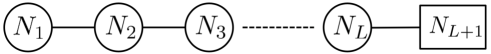
Figure 4: The quiver diagram for $T_{\rho}[SU(N)]$ with $\rho=(N_{1},N_{2}-N_{1},\cdots,N_{L+1}-N_{L})$ and $N:=N_{L+1}$. A circle with $N_{l}$ expresses the $\mathcal{N}=4$ $U(N_{l})$ vector multiplet. A line attached between two circles with $N_{l}$ and $N_{l+1}$ expresses an $\mathcal{N}=4$ bi-fundamental hypermultiplet. A line attached between the circle with $N_{L}$ and the box with $N_{L+1}$ represents $N_{L+1}$ $U(N_{L})$ fundamental hypermultiplets.

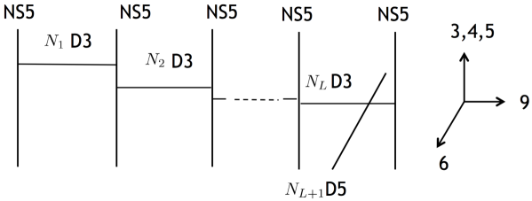
Figure 5: The brane configuration of $T_{\rho}[SU(N)]$. The vertical lines express NS5-branes and the horizontal lines express D3-branes.

One can introduce an FI term for each $U(1)$ factor of the gauge group. Each FI parameter is a triplet of $SU(2)_{H}$, which can be decomposed into one real and one complex FI parameters. Since we are interested in the half-BPS vortex solutions, which are in general allowed only for the vanishing complex FI parameters Bullimore:2016hdc , we only turn on the real FI parameters $(\xi_{1},\xi_{2},\cdots,\xi_{L})$ for the gauge group $\prod_{l=1}^{L}U(N_{l})$. The R-symmetry group $SU(2)_{C}\times SU(2)_{H}$ is broken to $SU(2)_{C}\times U(1)_{H}$ in the presence of the FI term.

In the brane setup, the nonzero real FI parameters are achieved by separations of the NS5-branes along the 6-direction. We also take the $N_{L+1}$ D5-branes to the right in the $9$-direction. When the D5-branes across the rightmost NS5-brane, the D3-brane annihilations and creations occur and $N_{L+1}-N_{L}$ D3-branes suspended between the rightmost NS5-brane and the D5-branes appear. Then we obtain a brane configuration sketched in figure 6. The magnitude of an FI parameter $\xi_{l}$ is proportional to the distance between $N_{l+1}-N_{l}$ D3-branes and $N_{l}-N_{l-1}$ D3-branes in the 6-direction.

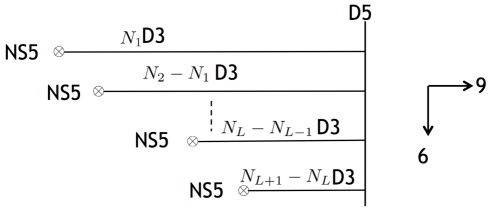
Figure 6: The brane configuration for a Higgs branch. The horizontal lines are D3-branes suspended between a NS5-brane and D5-branes. The distance between $N_{l+1}-N_{l}$ D3-branes and $N_{l}-N_{l-1}$ D3-branes along the $6$-direction is proportional to the magnitude of FI parameter $\xi_{l}$ of $U(N_{l})$.

The half-BPS vortices are engineered by $n_{l=1,\cdots,L}$ D1-branes stretched between D3-branes as shown in figure 7, where the world-volume of D1-branes are $06$-directions. By sending $N_{L+1}$ D5-branes to right infinity in the 9-direction, one can read off the world-volume theory of D1-branes, which is 1d $\mathcal{N}=4$ supersymmetric quiver quantum mechanics. The quiver diagram of the quantum mechanics is specified by figure 8. The closed loops of arrows in figure 8 correspond to the following superpotential terms:

$$W=\sum_{l=1}^{L-1}J_{l}C_{l}I_{l+1}+\sum_{l=1}^{L-1}\mathrm{Tr}B_{l}C_{l}A_{l}-\sum_{l=1}^{L-1}\mathrm{Tr}B_{l+1}A_{l}C_{l}$$ (31)

where $I_{l}$, $J_{l}$ and $B_{l}$ are $N_{l}-N_{l-1}$ fundamental, $N_{l+1}-N_{l}$ anti-fundamental and an adjoint chiral multiplets of a gauge group $U(n_{l})$, respectively. $A_{l}$ and $C_{l}$ are $U(n_{l})\times U(n_{l+1})$ bi-fundamental chiral multiplets. The moduli space of vortices is given by the D-term and F-term solution of the quiver quantum mechanics. The gauge coupling $e_{l}$ of 3d gauge group $U(N_{l})$ is related to the FI parameter $\zeta_{l}$ of 1d gauge group $U(n_{l})$ as $\zeta_{l}={2\pi}/{e^{2}_{l}}$.

The global symmetry group of the 1d $\mathcal{N}=4$ quantum mechanics is $[\prod_{l=1}^{L+1}U(N_{l}-N_{l-1})]/U(1)^{L}\times SU(2)_{C}\times U(1)_{H}\times U(1)_{Z}$, where $U(1)_{Z}$ is associated with the rotation in the 12-directions and $SU(2)_{C}\times U(1)_{H}$ is the R-symmetry group, which descends from the 3d R-symmetry. The diagonal combination $U(1)_{\epsilon}:=\mathrm{diag}(U(1)_{H}\times U(1)_{Z})$ commutes with the 1d supersymmetry and acts on each multiplet as a flavor symmetry Bullimore:2016hdc . The charge assignment is summarized in table 4.

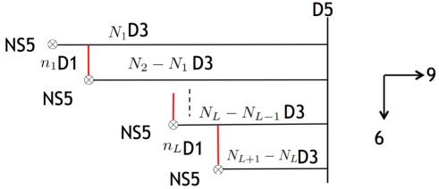
Figure 7: The brane configuration of the $(n_{1},n_{2},\cdots,n_{L})$ vortex. The vertical red lines express D1-branes.

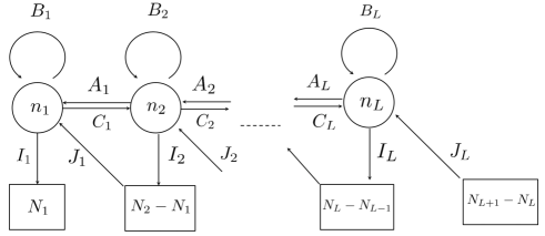
Figure 8: The quiver diagram for the $(n_{1},n_{2},\cdots,n_{L})$ vortex world-line theory. The circle with $n_{l}$ expresses the 1d $\mathcal{N}=4$ $U(n_{l})$ vector multiplet and the arrows express 1d $\mathcal{N}=4$ chiral multiplets. The box with $N_{l}-N_{l-1}$ expresses the number of chiral multiplets.

	$U(n_{l})$	$U(n_{l+1})$	$U(N_{l}-N_{l-1})$	$U(N_{l+1}-N_{l})$	$U(1)_{H}$	$U(1)_{\epsilon}$
$I_{l}$	$\mathbf{n_{l}}$	$\mathbf{1}$	$\mathbf{\overline{N_{l}-N_{l-1}}}$	$\mathbf{1}$	$0$	$-1$
$J_{l}$	$\mathbf{\overline{n_{l}}}$	$\mathbf{1}$	$\mathbf{1}$	$\mathbf{N_{l+1}-N_{l}}$	$0$	$-1$
$A_{l}$	$\mathbf{\overline{n_{l}}}$	$\mathbf{n_{l+1}}$	$\mathbf{1}$	$\mathbf{1}$	$0$	$0$
$B_{l}$	$\mathbf{\mathrm{adj}}$	$\mathbf{1}$	$\mathbf{1}$	$\mathbf{1}$	$0$	$-2$
$C_{l}$	$\mathbf{n_{l}}$	$\mathbf{\overline{n_{l+1}}}$	$\mathbf{1}$	$\mathbf{1}$	$2$	$2$

Table 4: The symmetry charges of the 1d $\mathcal{N}=4$ chiral multiplets we introduce. There is also the $SU(2)_{C}$ symmetry, which is a part of the 1d R-symmetry. All the multiplets in the table carry spin zero under this $SU(2)_{C}$, i.e., $J_{3}=0$.

Now we would like to compute the index of this vortex quantum mechanics. The refined Witten index of $\mathcal{N}=4$ handsaw quiver quantum mechanics is written as Hori:2014tda

$$I=\mathrm{Tr}\left[(-1)^{F}y^{R-2J_{3}}\prod_{a}x^{G^{(a)}_{F}}_{a}\right]$$ (32)

where $J_{3}$ is the Cartan generator of $SU(2)_{C}$ and $R$ is the generator of $U(1)_{H}$. $x_{a}$’s denote fugacities for the $[\prod_{l=1}^{L+1}U(N_{l}-N_{l-1})]/U(1)^{L}\times U(1)_{\epsilon}$ flavor symmetry. $G^{(a)}_{F}$ is the corresponding flavor charge for $x_{a}$. More explicitly, we set $y=e^{\mu}$ as well as the other flavor fugacities: $e^{\gamma}$ for $U(1)_{\epsilon}$ and $e^{m^{(l)}_{a}}$ $(a=1,\cdots,N_{l}-N_{l-1})$ for the Cartan part of $U(N_{l}-N_{l-1})$.

As discussed in the previous section, this refined Witten index is given by the following JK-residue:

$$I=\frac{1}{|\mathsf{W}|}\text{JK-Res}_{\eta=\zeta}\left[g(u)d^{r}u\right]$$ (33)

where

$$g(u) =\left(\frac{1}{2\sinh\frac{-2\mu}{2}}\right)^{\sum_{l=1}^{L}n_{l}}\prod_{l=1}^{L}\left(\prod_{i\neq j}^{n_{l}}\frac{\sinh\frac{u^{(l)}_{i}-u^{(l)}_{j}}{2}}{\sinh\frac{u^{(l)}_{i}-u^{(l)}_{j}-2\mu}{2}}\right)\left(\prod_{i,j=1}^{n_{l}}\frac{\sinh\frac{u^{(l)}_{i}-u^{(l)}_{j}-2\mu-2\gamma}{2}}{\sinh\frac{u^{(l)}_{i}-u^{(l)}_{j}-2\gamma}{2}}\right)$$

$$\quad\times\left(\prod_{i=1}^{n_{l+1}}\prod_{j=1}^{n_{l}}\frac{\sinh\frac{u^{(l+1)}_{i}-u^{(l)}_{j}-2\mu}{2}}{\sinh\frac{u^{(l+1)}_{i}-u^{(l)}_{j}}{2}}\right)\left(\prod_{i=1}^{n_{l+1}}\prod_{j=1}^{n_{l}}\frac{\sinh\frac{-u^{(l+1)}_{i}+u^{(l)}_{j}+2\gamma}{2}}{\sinh\frac{-u^{(l+1)}_{i}+u^{(l)}_{j}+2\mu+2\gamma}{2}}\right)$$

$$\quad\times\left(\prod_{i=1}^{n_{l}}\prod_{b=N_{l-1}}^{N_{l}}\frac{\sinh\frac{u^{(l)}_{i}-m_{b}-2\mu-\gamma}{2}}{\sinh\frac{u^{(l)}_{i}-m_{b}-\gamma}{2}}\right)\left(\prod_{j=1}^{n_{l}}\prod_{a=N_{l}}^{N_{l+1}}\frac{\sinh\frac{-u^{(l)}_{j}+m_{a}-2\mu-\gamma}{2}}{\sinh\frac{-u^{(l)}_{j}+m_{a}-\gamma}{2}}\right).$$ (34)

We have defined $n_{L+1}=0$. Since $g(u)$ has degenerate poles for general gauge ranks $n_{l}$, the JK-residue computation requires a constructive definition of the JK-residue called the flag method Benini:2013xpa , which is very complicated to do analytically. Instead we adopt a prescription for the selection of the contributing poles and conduct tests for the prescription numerically. Motivated by the honest computation for $L=1$ in section 4.2, we select the following poles:

$$u^{(l)}_{i}=m_{a}+(2k_{a}-1)\gamma,\qquad a\in\{1,\ldots,N_{l}\},\quad k_{a}\in\{1,\ldots,n^{(l)}_{a}\}$$ (35)

where $(n^{(l)}_{1},\ldots,n^{(l)}_{N_{l}})$ is a partition of $n_{l}$, i.e., an ordered set of $N_{l}$ nonnegative integers satisfying $\sum_{a=1}^{N_{l}}n^{(l)}_{a}=n_{l}$. Every pair $(a,k_{a})$ is assigned to one of $i=1,\ldots,n_{l}$ exactly once. Evaluating the residue at each pole, we have

$$I=$$

$$\prod_{l=1}^{L}\left(\prod_{a=1}^{N_{l+1}}\prod_{b=1}^{N_{l}}\prod_{k_{a}=1}^{n^{(l+1)}_{a}}\frac{\sinh\frac{m_{a}-m_{b}+2(n^{(l+1)}_{a}-k_{a})\gamma}{2}}{\sinh\frac{m_{a}-m_{b}-2\mu+2(n^{(l+1)}_{a}-k_{a})\gamma}{2}}\prod_{a,b=1}^{N_{l}}\prod_{k_{a}=1}^{n^{(l)}_{a}}\frac{\sinh\frac{m_{a}-m_{b}-2\mu+2(k_{a}-n^{(l)}_{b}-1)\gamma}{2}}{\sinh\frac{m_{a}-m_{b}+2(k_{a}-n^{(l)}_{b}-1)\gamma}{2}}\right)^{\prime}$$

$$\quad\times\left(\prod_{a=1}^{N_{l+1}}\prod_{b=1}^{N_{l}}\prod_{k_{b}=1}^{n^{(l)}_{b}}\frac{\sinh\frac{m_{a}-m_{b}-2\mu+2(n^{(l+1)}_{a}-k_{b})\gamma}{2}}{\sinh\frac{m_{a}-m_{b}+2(n^{(l+1)}_{a}-k_{b})\gamma}{2}}\prod_{a,b=1}^{N_{l}}\prod_{k_{b}=1}^{n^{(l)}_{b}}\frac{\sinh\frac{m_{a}-m_{b}+2(k_{b}-n^{(l)}_{b}-1)\gamma}{2}}{\sinh\frac{m_{a}-m_{b}-2\mu+2(k_{b}-n^{(l)}_{b}-1)\gamma}{2}}\right)^{\prime}$$ (36)

where ^′ denotes that the vanishing factors are omitted. The permutations among $u^{(l)}_{i}$’s give rise to factor $n_{l}!$, which cancels the Weyl group factor $|\mathsf{W}|$. The detailed computation of (3.1) is similar to that of the single gauge node case, which is explicitly described in section 4.2. Using

$$(a;q)_{n-m}=\frac{(aq^{-m};q)_{n}}{(aq^{-m};q)_{m}},$$ (37)

(3.1) is further simplified such that the final expression of the index is given by

$$I=$$

$$\prod_{l=1}^{L}\left(\prod_{a,b=1}^{N_{l}}\prod_{k=1}^{n^{(l)}_{a}-n^{(l)}_{b}}\frac{\sinh\frac{m_{a}-m_{b}-2\mu+2(k-1)\gamma}{2}}{\sinh\frac{m_{a}-m_{b}+2(k-1)\gamma}{2}}\right)\left(\prod_{a=1}^{N_{l+1}}\prod_{b=1}^{N_{l}}\prod_{k=1}^{n^{(l)}_{b}-n^{(l+1)}_{a}}\frac{\sinh\frac{m_{a}-m_{b}-2\mu-2k\gamma}{2}}{\sinh\frac{m_{a}-m_{b}-2k\gamma}{2}}\right),$$ (38)

which agrees with the vortex partition function of $T_{\rho}[SU(N)]$ obtained in Bullimore:2014awa using the factorization of the $S^{3}_{b}$ partition function. We also conduct the numerical computation of (33) using the flag method and confirm that it agrees with (3.1).

3.2 $\mathcal{N}=2$ linear quiver gauge theories

Now we would like to extend our discussion of vortex quantum mechanics to 3d $\mathcal{N}=2$ linear quiver gauge theories. Unlike $T_{\rho}[SU(N)]$, the brane setup of an $\mathcal{N}=2$ linear quiver theory is in general not known. Thus, one cannot directly read off vortex quantum mechanics from the brane setup. Here, instead, we take an indirect approach: we first consider the $\mathcal{N}=2$ deformation of the previous $\mathcal{N}=4$ $T_{\rho}[SU(N)]$ example. Figure 9 represents $T_{\rho}[SU(N)]$ in terms of $\mathcal{N}=2$ multiplets.

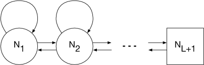
Figure 9: The quiver diagram representation of $T_{\rho}[SU(N)]$ is illustrated in terms of $N=2$ multiplets. A round node represents a gauge group factor with a corresponding $\mathcal{N}=2$ vector multiplet. Each arrow represents an $\mathcal{N}=2$ chiral multiplet in the bi-fundamental representation between the gauge group factors connected by the arrow. A square node represents flavor group factor.

In general, one can deform a 3d theory by turning on real mass for a global symmetry. Here we turn on real mass for the $U(1)_{A}$ symmetry, which is the off-diagonal combination of two $SU(2)$ R-symmetries. Since this real mass breaks the R-symmetry $SU(2)^{2}$ to $U(1)_{R}\times U(1)_{A}$ where $U(1)_{A}$ is a non-$R$ global symmetry, the deformed theory only preserves $\mathcal{N}=2$ supersymmetry. In addition, we also turn on the vacuum expectation values of vector multiplet scalars such that only the right-directed chiral multiplets in figure 9 remain massless. Thus, the deformed theory is given by figure 10.

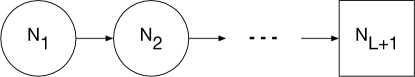
Figure 10: The quiver diagram representation of the 3d $\mathcal{N}=2$ theory deformed from $T_{\rho}[SU(N)]$. The deformed theory also includes various CS/BF interactions.

We emphasize that this deformation of $T_{\rho}[SU(N)]$ incorporates various CS/BF interactions in the deformed $\mathcal{N}=2$ theory. First, the fermions in the left-directed bi-fundamental chiral multiplets, which are integrated out, leave their remnants as the CS/BF interactions of levels

$$\begin{gathered}\kappa^{(l)}=\frac{N_{l-1}+N_{l+1}}{2},\\ \kappa_{U(1)}^{(l,l+1)}=-\frac{1}{2}\end{gathered}$$ (41)

where we have defined $N_{0}=0$. $\kappa^{(l)}$ is the CS level for the $l$-th gauge node and $\kappa_{U(1)}^{(l,l+1)}$ is the BF level between the $U(1)$ factors of the $l$-th and $(l+1)$-th gauge nodes. The $U(1)$ BF level is normalized such that the corresponding Lagrangian term is given by

$$\frac{\kappa_{U(1)}^{(l,l+1)}}{2\pi}\mathrm{Tr}A^{(l)}d\mathrm{Tr}A^{(l+1)}.$$ (42)

Second, the fermions in adjoint chiral multiplets, which are parts of the $\mathcal{N}=4$ vector multiplets, also give CS interactions but only for the $SU(N)$ parts:

$$\kappa^{(l)}_{SU(N)}=-N_{l}.$$ (43)

Combining (41) and (43), the induced CS/BF levels by the deformation are as follows:

$$\begin{gathered}\kappa^{(l)}=\frac{N_{l-1}+N_{l+1}}{2}-N_{l},\\ \Delta\kappa_{U(1)}^{(l)}=1,\\ \kappa_{U(1)}^{(l,l+1)}=-\frac{1}{2}\end{gathered}$$ (47)

with $N_{0}=0$. For later convenience, we organize the $SU(N)$ and $U(1)$ CS levels such that they are given by $U(N)$ CS levels, $\kappa^{(l)}$, and additional level shifts for the $U(1)$ parts, $\Delta\kappa_{U(1)}^{(l)}$. Again $\kappa_{U(1)}^{(l,l+1)}$ is the BF level between the $l$-th and $(l+1)$-th gauge nodes.

We have realized the $\mathcal{N}=2$ deformation of $T_{\rho}[SU(N)]$ by turning on real mass associated with the $U(1)_{A}$ symmetry, which is the off-diagonal combination of $SU(2)_{C}\times SU(2)_{H}$. The 3d $SU(2)_{C}\times SU(2)_{H}$ R-symmetry is broken to $SU(2)_{C}\times U(1)_{H}$ for nonzero 3d FI parameters and descends down to the 1d R-symmetry of vortex quantum mechanics. We have denoted the (Cartan) generators of 1d $SU(2)_{C}\times U(1)_{H}$ R-symmetry by $J_{3}$ and $R$. The 1d version of the $U(1)_{A}$ symmetry is thus generated by $R-2J_{3}$, whose mass parameter is denoted by $\mu$. Recall that the charges of the 1d multiplets are summarized in table 4. Each $\mathcal{N}=4$ chiral multiplet of $R-2J_{3}=r$ is decomposed into an $\mathcal{N}=2$ chiral of $R-2J_{3}=r$ and an $\mathcal{N}=2$ fermi of $R-2J_{3}=r-2$. Thus, one can read off the $\mathcal{N}=2$ chiral/fermi multiplets charged under $U(1)_{A}$, which become massive under the deformation $\mu\rightarrow\infty$. After integrating them out, the remaining quantum mechanics is given by figure 11.

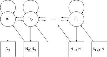
Figure 11: The quiver diagram representation of vortex quantum mechanics for the $\mathcal{N}=2$ deformed theory of $T_{\rho}[SU(N)]$.

Note that the integrated out 1d multiplets leave their remnants as Wilson lines in quantum mechanics. First, the fundamental and anti-fundamental fermi multiplets induce the following gauge/global Wilson lines:

$$\prod_{l=1}^{L}e^{q_{l}\sum_{i=1}^{n_{l}}u^{(l)}_{i}+\frac{1}{2}n_{l}\sum_{a=N_{l-1}+1}^{N_{l}}m_{a}-\frac{1}{2}n_{l}\sum_{a=N_{l}+1}^{N_{l+1}}m_{a}}$$ (48)

where the gauge Wilson line charge,

$$q_{l}=\frac{N_{l-1}+N_{l+1}}{2}-N_{l},$$ (49)

coincides with the CS level $\kappa^{(l)}$ of the 3d theory. Second, the bi-fundamental chiral and fermi multiplets that are integrated out induce the following global Wilson lines:

$$\prod_{l=1}^{L-1}e^{-n_{l}n_{l+1}\gamma}.$$ (50)

Last, the adjoint chiral and fermi multiplets that are integrated out induce global Wilson lines

$$\prod_{l=1}^{L}e^{n_{l}^{2}\gamma}.$$ (51)

Those gauge/global Wilson lines should be the quantum mechanics counterparts of the CS/BF interactions in the deformed 3d theory. By comparing them with the result from the factorization of the 3d topologically twisted index, which is shown in appendix A, one can identify the 3d origin of each Wilson line. It turns out that the 3d CS/BF interactions of the levels (47) have their Wilson line counterparts in quantum mechanics as follows:

$$\begin{gathered}\prod_{l=1}^{L}e^{\kappa^{(l)}\sum_{i=1}^{n_{l}}u^{(l)}_{i}},\\ \prod_{l=1}^{L}e^{\Delta\kappa_{U(1)}^{(l)}(n_{l}^{2}\gamma+n_{l}\sum_{a=1}^{N_{l}}m_{a})},\\ \prod_{l=1}^{L-1}e^{\kappa_{U(1)}^{(l,l+1)}(2n_{l}n_{l+1}\gamma+n_{l}\sum_{a=1}^{N_{l+1}}m_{a}+n_{l+1}\sum_{a=1}^{N_{l}}m_{a})}\end{gathered}$$ (55)

where we have used $\sum_{a=1}^{N_{L+1}}m_{a}=0$, the traceless condition for $SU(N_{L+1})$. Indeed, from the factorization result, we expect that (55) is not restricted to the specific levels in (47) but is generally applicable. Thus, we conclude that a 3d $\mathcal{N}=2$ linear quiver gauge theory of figure 10 with CS/BF levels $\kappa^{(l)}$, $\Delta\kappa_{U(1)}^{(l)}$ and $\kappa_{U(1)}^{(l,l+1)}$ has vortex quantum mechanics of figure 11 with the Wilson lines (55). Those Wilson lines will play important roles when we discuss Seiberg-like dualities for $\mathcal{N}=2$ linear quiver theories in the next section.

Next we move on to the index of this vortex quantum mechanics. The refined Witten index is given by

$$I=\frac{1}{|\mathsf{W}|}\text{JK-Res}_{\eta=\zeta}\left[g(u)d^{r}u\right]$$ (56)

where $g(u)$ is now written as

$$g(u) =W(u)\prod_{l=1}^{L}\frac{\left(\prod_{i\neq j}^{n_{l}}\sinh\frac{u^{(l)}_{i}-u^{(l)}_{j}}{2}\right)\left(\prod_{i=1}^{n_{l+1}}\prod_{j=1}^{n_{l}}\sinh\frac{u^{(l+1)}_{i}-u^{(l)}_{j}-2\gamma}{2}\right)}{\left(\prod_{i,j=1}^{n_{l}}\sinh\frac{u^{(l)}_{i}-u^{(l)}_{j}-2\gamma}{2}\right)\left(\prod_{i=1}^{n_{l+1}}\prod_{j=1}^{n_{l}}\sinh\frac{u^{(l+1)}_{i}-u^{(l)}_{j}}{2}\right)}$$

$$\qquad\times\frac{1}{\left(\prod_{i=1}^{n_{l}}\prod_{b=N_{l-1}+1}^{N_{l}}\sinh\frac{u^{(l)}_{i}-m_{b}-\gamma}{2}\right)\left(\prod_{j=1}^{n_{l}}\prod_{a=N_{l}+1}^{N_{l+1}}\sinh\frac{-u^{(l)}_{j}+m_{a}-\gamma}{2}\right)}$$ (57)

with $n_{L+1}=0$. $W(u)$ is the Wilson line contribution given by the product of the three factors in (55). We adopt the same prescription as in $T_{\rho}[SU(N)]$ which selects the following poles contributing to the index:

$$u^{(l)}_{i}=m_{a}+(2k_{a}-1)\gamma,\qquad a\in\{1,\ldots,N_{l}\},\quad k_{a}\in\{1,\ldots,n^{(l)}_{a}\}.$$ (58)

$(n^{(l)}_{1},\ldots,n^{(l)}_{N_{l}})$ is a partition of $n_{l}$ into $N_{l}$ nonnegative integers. Again every pair $(a,k_{a})$ is assigned to one of $i=1,\ldots,n_{l}$ exactly once. Along the same computations as in $T_{\rho}[SU(N)]$, the final expression of the index is obtained as follows:

$$I =W\prod_{l=1}^{L}\left(\prod_{a\neq b}^{N_{l}}\prod_{k=1}^{n^{(l)}_{a}-n^{(l)}_{b}}\sinh\frac{m_{a}-m_{b}+2(k-1)\gamma}{2}\right)^{-1}$$

$$\qquad\times\left(\prod_{a=1}^{N_{l+1}}\prod_{b=1}^{N_{l}}\prod_{k=1}^{n^{(l)}_{b}-n^{(l+1)}_{a}}\sinh\frac{m_{a}-m_{b}-2k\gamma}{2}\right)^{-1}$$ (59)

where the Wilson line contribution $W$ is given by

$$W =\prod_{l=1}^{L}e^{\kappa^{(l)}\sum_{a=1}^{N_{l}}(n^{(l)}_{a}m_{a}+n^{(l)}_{a}{}^{2}\gamma)}e^{\Delta\kappa_{U(1)}^{(l)}(n_{l}^{2}\gamma+n_{l}\sum_{a=1}^{N_{l}}m_{a})}$$

$$\quad\times e^{\kappa_{U(1)}^{(l,l+1)}(2n_{l}n_{l+1}\gamma+n_{l}\sum_{a=1}^{N_{l+1}}m_{a}+n_{l+1}\sum_{a=1}^{N_{l}}m_{a})}.$$ (60)

We also conduct the numerical computation of (56) using the flag method Benini:2013xpa and confirm that it agrees with (3.2). Indeed, (3.2) agrees with (255), the vortex partition function obtained from the factorization of the 3d topologically twisted index.

We have seen that the index of quantum mechanics in figure 11 gives the vortex partition function of the 3d linear quiver gauge theory in figure 10, which is also obtained from the factorization of a 3d supersymmetric partition function. Introducing 2d parameters $m^{\text{2d}}_{a}=r^{-1}m_{a},\gamma^{\text{2d}}=r^{-1}\gamma$, one can also consider the 2d reduction of the 3d vortex partition function, which is equivalent to (3.2), by taking the limit $r\rightarrow 0$. We observe that the 2d reduction of (3.2) correctly reproduces the known 2d vortex partition function Nawata:2014nca . This is another evidence that quantum mechanics in figure 11 describes vortices of the 3d theory in figure 10. Moreover, one should note that nontrivial Wilson lines are allowed in the quantum mechanics description. We have fine-tuned those Wilson lines so that they correctly reflect CS/BF interactions of the parent 3d theory.

We comment on mathematical aspects of the world volume theory of vortices. The type of a quiver in figure 11 is called a ‘hand-saw’ quiver, which is isomorphic to a parabolic Laumon space Finkelberg2014 . The parabolic Laumon space coincides with the moduli space of based quasi maps $\mathbf{P}^{1}$ into the flag variety. The precise relation between quasimaps and the moduli space of vortex equation was studied in Venugopalan2013 . The equivariant integrations over the based quasi map spaces give the equivariant J-function of the flag variety, which is the 2d reduction of vortex partition function. Then our construction of vortex quantum mechanics is regarded as K-theoretic uplift. The index of vortex quantum mechanics with a particular choice of Wilson lines reproduces the K-theoretic J-function.

4 Vortices and Seiberg-like dualities

4.1 $\mathcal{N}=2$ SQCDs

We have constructed 1d quantum mechanical systems which describe the low energy dynamics of vortices in 3d linear quiver theories. The moduli space of vortices is given by the Higgs branch of such vortex quantum mechanics. We have also computed the refined Witten indices of vortex quantum mechanics, which can be identified as the partition functions of vortices on $\Omega$-deformed $\mathbb{R}^{2}_{\Omega}\times S^{1}$. In this section, using these vortex partition functions, we examine how vortex quantum mechanics behave under 3d Seiberg-like dualities we reviewed in section 2.1.

The example we discuss in this section is the $\mathcal{N}=2$ $U(N_{c})_{\kappa}$ gauge theory with $N_{f}$ fundamental chiral multiplets and $N_{a}$ anti-fundamental chiral multiplets. We include the Chern-Simons interaction with level $|\kappa|\leq\frac{|N_{f}-N_{a}|}{2}$ and FI parameter $\xi$. We assume $N_{f}\geq N_{a}$ and $\xi>0$. The ranges of $\kappa$ and $\xi$ are restricted such that the theory only has Higgs vacua and avoids topological vacua as we discuss in section 2.1. The original Aharony duality and its generalizations tell us that this theory has a dual description, $U(N_{f}-N_{c})_{-\kappa}$ gauge theory with $(N_{a},N_{f})$ flavors and extra gauge singlet fields described in section 2.1 Aharony:1997gp ; Benini:2011mf .

In order to understand the effect of the Aharony duality on vortex quantum mechanics, we first consult the brane picture. Recall the brane setup and the motion representing the Aharony duality, which are illustrated in figure 1. Now we insert additional D1-branes ending on D3-branes, which correspond to the presence of vortices in the 3d theory. The brane motion in the presence of D1-branes is illustrated in figure 12.

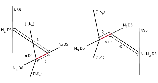
Figure 12: The brane motion representing the Aharony duality in the presence of vortices. Vortices are realized as D1-branes denoted by the red line in the figure. The length of the D1-branes corresponds to 3d FI parameter $\xi$ while the length of the D3-branes corresponds to 1d FI parameter $\zeta$. The spacetime directions occupied by each brane are summarized in table 5.

Branes	0	1	2	3	4	5	6	7	8	9
NS5	$\times$	$\times$	$\times$	$\times$	$\times$	$\times$
$(1,k_{\pm})$	$\times$	$\times$	$\times$			$\cdot$	$\cdot$	$\times$	$\times$
D5	$\times$	$\times$	$\times$				$\times$	$\times$	$\times$
D3	$\times$	$\times$	$\times$							$\times$
D1	$\times$						$\times$

Table 5: The spacetime directions occupied by the branes in figure 12 are marked by $\times$. The $(1,k_{\pm})$-branes occupy 1-dimensional subspaces in the 56-plane.

One can see that the brane motion is controlled by the relative distance between the NS5-brane and the $(1,k_{\pm})$-branes along the 9-direction. In the 3d theory point of view, this distance is proportional to the inverse of the gauge coupling squared, $1/g^{2}$. The position that the NS5-brane and the $(1,k_{\pm})$-branes are exchanged is therefore the infinite-coupling point, which is consistent with the fact the Aharony duality is an IR duality where 3d theories strongly interact.

On the other hand, in the vortex quantum mechanics point of view, that distance corresponds to Fayet-Iliopoulos parameter $\zeta$. Especially, the position exchanging the NS5-brane and the $(1,k_{\pm})$-branes corresponds to $\zeta=0$ where a non-compact Coulomb branch of the quantum mechanics can appear depending on the values of $k_{\pm}=\kappa\pm\frac{N_{f}-N_{a}}{2}$. In figure 12, the NS5-brane and the $(1,k_{\pm})$-branes have the common 9-direction coordinate when $\zeta=0$. Thus, D1-branes can be suspended between them. When either $k_{\pm}=0$, we have two NS5-branes sharing a (semi-)infinite parallel direction, which allows the D1-branes to move along that direction. Thus, the D1-brane theory has a flat direction at $\zeta=0$, which we call a Coulomb branch. Due to the appearance of the flat direction, some states of vortex quantum mechanics can escape through the flat direction such that a jump of the spectrum can happen at $\zeta=0$. This phenomenon is called the wall-crossing. The important point is that the wall-crossing of vortex quantum mechanics and the Aharony duality of the 3d theory are inferred from the same brane motion.

From the brane picture, we expect that vortex quantum mechanics experiences the shift of the FI parameter from $\zeta>0$ to $\zeta<0$, and possibly the nontrivial wall-crossing at $\zeta=0$, under the Seiberg-like duality of the parent 3d theory. We now validate this expectation by the explicit computations of the quantum mechanics indices for different 1d FI parameters. For the 3d $\mathcal{N}=2$ $U(N_{c})_{\kappa}$ theory with $(N_{f},N_{a})$ flavors, the moduli space of $n$ vortices is described by the $\mathcal{N}=2$ gauged quantum mechanics illustrated in figure 13 Fujitsuka:2013fga .

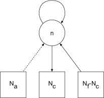
Figure 13: The quiver diagram representation of vortex quantum mechanics for the 3d $\mathcal{N}=2$ $U(N_{c})_{\kappa}$ theory with $(N_{f},N_{a})$ flavors. A solid arrow denotes a 1d $\mathcal{N}=2$ chiral multiplet while a dashed arrow denotes a 1d $\mathcal{N}=2$ fermi multiplet.

The refined Witten index of this quantum mechanics is given by

$$I^{n}=\frac{1}{|\mathsf{W}|}\text{JK-Res}_{\eta=\zeta}\left[g^{n}(u)d^{n}u\right]$$ (61)

where $|\mathsf{W}|=n!$ is the Weyl group order of the gauge group $U(n)$ and

$$g^{n}(u)=$$

$$\frac{e^{\kappa\sum_{i=1}^{n}u_{i}}\left(\prod_{i\neq j}^{n}\sinh\frac{u_{i}-u_{j}}{2}\right)\left(\prod_{j=1}^{n}\prod_{a=1}^{N_{a}}\sinh\frac{-u_{j}+\tilde{m}_{a}-\mu+\gamma}{2}\right)}{\left(\prod_{i,j=1}^{n}\sinh\frac{u_{i}-u_{j}-2\gamma}{2}\right)\left(\prod_{i=1}^{n}\prod_{b=1}^{N_{c}}\sinh\frac{u_{i}-m_{b}-\mu-\gamma}{2}\right)\left(\prod_{j=1}^{n}\prod_{a=N_{c}+1}^{N_{f}}\sinh\frac{-u_{j}+m_{a}+\mu-\gamma}{2}\right)}$$ (62)

is the integrand given by the classical action and the 1-loop determinant. We have made shifts of mass parameters $m\rightarrow m+\mu$, $\tilde{m}\rightarrow\tilde{m}-\mu$ where $\mu$ is associated with the $U(1)_{A}$ symmetry rotating the 3d fundamental and anti-fundamental fields simultaneously. Note that we have chosen the auxiliary JK-vector $\eta=\zeta$ such that asymptotic poles do not participate. We want to compare the indices of this vortex quantum mechanics for different FI parameters: $\zeta>0$ and $\zeta<0$.

Let us consider the $\zeta>0$ case first. The JK-residue rule chooses sets of linearly independent hyperplanes in $\mathbb{R}^{n}$ such that a chosen set of hyperplanes determine each $u_{i}$ as follows:

$$u_{i}=\left\{\begin{array}[]{l}m_{a}+\mu+\gamma,\qquad a\in\{1,\ldots,N_{c}\}\\ u_{j}+2\gamma.\end{array}\right.$$ (65)

The pole determined by the intersection of those hyperplanes is given by

$$u_{i}=m_{a}+\mu+(2k_{a}-1)\gamma,\qquad a\in\{1,\ldots,N_{c}\},\quad k_{a}\in\{1,\ldots,n_{a}\}$$ (66)

where $(n_{1},\ldots,n_{N_{c}})$ is a partition of $n$, i.e., an ordered set of $N_{c}$ nonnegative integers satisfying $\sum_{a=1}^{N_{c}}n_{a}=n$. Every pair $(a,k_{a})$ is assigned to one of $i=1,\ldots,n$ exactly once. Evaluating the residue at this pole, we have

$$\frac{e^{\kappa\sum_{a=1}^{N_{c}}\sum_{k_{a}=1}^{n_{a}}(m_{a}+\mu+(2k_{a}-1)\gamma)}\left(\prod_{a,b=1}^{N_{c}}\prod_{k_{a}=1}^{n_{a}}\prod_{k_{b}=1}^{n_{b}}\sinh\frac{m_{a}-m_{b}+2(k_{a}-k_{b})\gamma}{2}\right)^{\prime}}{\left(\prod_{a,b=1}^{N_{c}}\prod_{k_{a}=1}^{n_{a}}\prod_{k_{b}=1}^{n_{b}}\sinh\frac{m_{a}-m_{b}+2(k_{a}-k_{b}-1)\gamma}{2}\right)^{\prime}\left(\prod_{a=1}^{N_{c}}\prod_{k_{a}=1}^{n_{a}}\prod_{b=1}^{N_{c}}\sinh\frac{m_{a}-m_{b}+2(k_{a}-1)\gamma}{2}\right)^{\prime}}$$

$$\times\frac{\left(\prod_{a=1}^{N_{a}}\prod_{b=1}^{N_{c}}\prod_{b=1}^{n_{b}}\sinh\frac{\tilde{m}_{a}-m_{b}-2\mu-2(k_{b}-1)\gamma}{2}\right)}{\left(\prod_{a=N_{c}+1}^{N_{f}}\prod_{b=1}^{N_{c}}\prod_{k_{b}=1}^{n_{b}}\sinh\frac{m_{a}-m_{b}-2k_{b}\gamma}{2}\right)}$$ (67)

where ^′ denotes that the vanishing factors are omitted. The permutations among $u_{i}$’s give rise to factor $n!$, which cancels the Weyl group factor $|\mathsf{W}|$. The first line of (4.1) is simplified to

$$\frac{(-1)^{nN_{c}}e^{\kappa\sum_{a=1}^{N_{c}}(n_{a}m_{a}+n_{a}\mu+n_{a}^{2}\gamma)}}{\left(\prod_{a,b=1}^{N_{c}}\prod_{k_{b}=1}^{n_{b}}\sinh\frac{m_{a}-m_{b}-2(k_{b}-n_{a}-1)\gamma}{2}\right)}.$$ (68)

Combined with the second line of (4.1), it reproduces the known vortex partition function of 3d $\mathcal{N}=2$ $U(N_{c})_{\kappa}$ theory with $(N_{f},N_{a})$ flavors on $\Omega$-deformed $\mathbb{R}_{\Omega}^{2}\times S^{1}$ Hwang:2012jh :

$$\frac{(-1)^{nN_{c}}e^{\kappa\sum_{a=1}^{N_{c}}(n_{a}m_{a}+n_{a}\mu+n_{a}^{2}\gamma)}\left(\prod_{a=1}^{N_{a}}\prod_{b=1}^{N_{c}}\prod_{k_{b}=1}^{n_{b}}\sinh\frac{\tilde{m}_{a}-m_{b}-2\mu-2(k_{b}-1)\gamma}{2}\right)}{\left(\prod_{a,b=1}^{N_{c}}\prod_{k_{b}=1}^{n_{b}}\sinh\frac{m_{a}-m_{b}-2(k_{b}-n_{a}-1)\gamma}{2}\right)\left(\prod_{a=N_{c}+1}^{N_{f}}\prod_{b=1}^{N_{c}}\prod_{k_{b}=1}^{n_{b}}\sinh\frac{m_{a}-m_{b}-2k_{b}\gamma}{2}\right)}$$ (69)

up to sign, which can be absorbed to the vorticity fugacity.

Next let us examine the $\zeta<0$ case. Since different $\eta$ is used, different sets of hyperplanes are chosen by the JK-residue rule. Now a set of hyperplanes chosen by the JK-residue rule determine each $u_{i}$ as follows:

$$u_{i}=\left\{\begin{array}[]{l}m_{a}+\mu-\gamma,\qquad a\in\{N_{c}+1,\ldots,N_{f}\}\\ u_{j}-2\gamma.\end{array}\right.$$ (72)

Thus, we evaluate the residue at pole

$$u_{i}=m_{a}+\mu-(2k_{a}-1)\gamma,\qquad\begin{array}[]{l}a\in\{N_{c}+1,\ldots,N_{f}\},\\ k_{a}\in\{1,\ldots,n_{a}\},\\ n_{a}\geq 0,\quad\sum_{a=N_{c}+1}^{N_{f}}n_{a}=n\end{array}$$ (76)

and obtain the following result:

$$(-1)^{n(N_{c}-N_{f}+N_{a})}e^{-\kappa\sum_{a=N_{c}+1}^{N_{f}}\sum_{k_{a}=1}^{n_{a}}(-n_{a}m_{a}-n_{a}\mu+n_{a}^{2}\gamma)}\times$$

$$\frac{\left(\prod_{a=1}^{N_{a}}\prod_{b=N_{c}+1}^{N_{f}}\prod_{k_{b}=1}^{n_{b}}\sinh\frac{-\tilde{m}_{a}+m_{b}+2\mu-2k_{b}\gamma}{2}\right)}{\left(\prod_{a,b=N_{c}+1}^{N_{f}}\prod_{k_{b}=1}^{n_{b}}\sinh\frac{-m_{a}+m_{b}-2(k_{b}-n_{a}-1)\gamma}{2}\right)\left(\prod_{a=N_{c}+1}^{N_{f}}\prod_{k_{a}=1}^{n_{a}}\prod_{b=1}^{N_{c}}\sinh\frac{-m_{b}+m_{a}-2k_{a}\gamma}{2}\right)},$$ (77)

which, up to sign, is the vortex partition function of the dual $U(N_{f}-N_{c})_{-\kappa}$ theory with $(N_{a},N_{f})$ flavors Hwang:2012jh ; Hwang:2015wna . Thus, by the explicit computations of the quantum mechanics indices for different $\zeta$, we have shown that the Aharony duality of a 3d $\mathcal{N}=2$ SQCD corresponds to the sign flip of the FI parameter in vortex quantum mechanics.

As discussed at the beginning of the section, the shift of the FI parameter from $\zeta>0$ to $\zeta<0$ may accompany a nontrivial jump of the spectrum at $\zeta=0$, which is called wall-crossing, depending on $N_{f}$, $N_{a}$ and $\kappa$. In the context of the JK-residue, such a jump of the index can happen if we have nontrivial residue contributions from asymptotic regions. The existence of an asymptotic pole is a signal of a non-compact Coulomb branch. From (4.1), one can find a necessary condition for nontrivial residues at asymptotic regions by taking one $u_{i}$ very large, $u_{i}\rightarrow\pm\infty$:

$$g^{n}(u)\sim e^{\left(\kappa\pm\frac{N_{a}-N_{f}}{2}\right)u_{i}}.$$ (78)

This should not vanish in order to have nontrivial residues at asymptotic regions. A necessary condition is thus

$$\pm(\kappa\pm\frac{N_{a}-N_{f}}{2})=\pm\kappa-\frac{N_{f}-N_{a}}{2}\geq 0.$$ (79)

Since we only allow $|\kappa|\leq\frac{|N_{f}-N_{a}|}{2}$, a relevant condition is the following:

$$\pm\kappa-\frac{N_{f}-N_{a}}{2}=0.$$ (80)

This is the same condition that the 3d theory has non-compact Coulomb branches Benini:2011mf . In the brane picture, this condition implies that there is an infinite parallel direction shared by two NS5-branes, along which D3-branes or D1-branes can move. These moduli of D3-branes and D1-branes are exactly their non-compact Coulomb branches. Therefore, there can be nontrivial wall-crossing of vortex quantum mechanics if the 3d theory has a non-compact Coulomb branch.

Now we should ask if this necessary condition is also sufficient. We show that it is the case by the explicit computation of the wall-crossing spectrum. Let us consider the 1-vortex case first. Recall that the vortex quantum mechanics index is given by (61). Since the theory is now a rank-1 theory,

$$I_{\zeta>0}=\text{JK-Res}_{\eta=\zeta}\left[g(u)du\right]=\sum_{Q(u*)>0}\mathrm{Res}_{u=u*}\left[g(u)du\right]$$ (81)

where the residues are summed over the poles whose corresponding charges are positive. Indeed, the JK-residue is independent of the choice of $\eta$. Thus, one can also take $\eta=-\zeta$, in which case asymptotic poles also contribute:

$$I_{\zeta>0} =\text{JK-Res}_{\eta=-\zeta}\left[g(u)du\right]$$

$$=-\sum_{Q(u*)<0}\mathrm{Res}_{u=u*}\left[g(u)du\right]-\mathrm{Res}_{u=\pm\infty}\left[g(u)du\right].$$ (82)

Note that the first term in the last line is nothing but the index with $\zeta<0$. Thus, as discussed, there is a jump between $I_{\zeta>0}$ and $I_{\zeta<0}$ if we have the nonzero asymptotic residue contribution. From (80) the asymptotic poles are simple if they exist. One can compute their residues as follows:

$$-\mathrm{Res}_{u=\pm\infty}\left[g(u)du\right] =\lim_{u\rightarrow\infty}g(u)-\lim_{u\rightarrow-\infty}g(u)$$ (83)

$$=\delta_{2\kappa,N_{f}-N_{a}}\frac{(-1)^{N_{a}-N_{f}+N_{c}}e^{\frac{N_{f}+N_{a}}{2}\mu+(N_{c}-\frac{N_{f}+N_{a}}{2})\gamma}}{\sinh(-\gamma)}$$

$$\quad-\delta_{2\kappa,N_{a}-N_{f}}\frac{(-1)^{-N_{c}}e^{-\frac{N_{f}+N_{a}}{2}\mu-(N_{c}-\frac{N_{f}+N_{a}}{2})\gamma}}{\sinh(-\gamma)}.$$ (84)

It shows that there is the nontrivial wall-crossing if and only if the condition (80) is met. Also we emphasize that (84) agrees with the 1-particle BPS index of $V_{\pm}$ Hwang:2012jh ; Hwang:2015wna , which are extra neutral chiral fields on the dual side describing the Coulomb branches of the 3d theory. We will see shortly that the whole wall-crossing factor incorporating multi-vortices is given by the Plethystic exponential of (84).

Now let us move on to multi-vortices cases. We first consider the following case:

$$\kappa=\frac{N_{f}-N_{a}}{2}\neq 0.$$ (85)

There is a pole at $u_{i}\rightarrow\infty$ and no pole at $u_{i}\rightarrow-\infty$. Recall that the poles chosen by the JK-residue rule with $\eta=\zeta>0$ are given by (66). One can see that those poles are exactly the poles contributing to the contour integral with the unit circle contour. See Hwang:2015wna for example. In other words, the JK-residue (61) can be rewritten in the following way:

$$I^{n}_{\zeta>0}=\frac{1}{|\mathsf{W}|}\text{JK-Res}_{\eta=\zeta}\left[g^{n}(u)d^{n}u\right]=\frac{1}{|\mathsf{W}|}\oint_{|z_{i}|=1}\frac{d^{n}z}{\prod_{i=1}^{n}z_{i}}g^{n}(\log z)$$ (86)

where $z_{i}=e^{u_{i}}$ and we assume that $\mathrm{Re}(\mu)=\mathrm{Re}(m_{a})=0$ while $\mathrm{Re}(\gamma)<0$. The contour is taken to be the unit circle traversed counterclockwise. One can check equation (86) by applying the residue theorem and taking the residues from the inside of the unit circle. On the other hand, one can also evaluate the same integral by taking the residues from the outside of the unit circle. In that case, a contributing pole is determined by a set of hyperplanes:

$$z_{i} =\left\{\begin{array}[]{l}t_{a}\tau x^{-1},\\ \infty,\\ z_{j}x^{-2}\end{array}\right.$$ (90)

where $t_{a}=e^{m_{a}}$, $\tau=e^{\mu}$ and $x=e^{\gamma}$.

At the pole, each $z_{i}$ takes either a finite value or an asymptotic value. One can decompose the hyperplanes (90) into two sets:

$$\{H_{1},\ldots,H_{m}\}\cup\{H_{m+1},\ldots,H_{n}\}$$ (91)

such that $\{H_{1},\ldots,H_{k}\}$ determines a set of $z_{i}$’s who take asymptotic values at the pole while $\{H_{k+1},\ldots,H_{n}\}$ determines the other set of $z_{i}$’s who take finite values at the pole. Let us define $I$ and $J$, two sets of gauge indices, such that $z_{i}$ is determined by $\{H_{1},\ldots,H_{m}\}$ if $i\in I$ and is determined by $\{H_{m+1},\ldots,H_{n}\}$ if $i\in J$. Now we decompose the integrand into three parts:

$$g^{n}(u)=$$

$$\frac{e^{\kappa\sum_{i\in I}u_{i}}\left(\prod_{i\neq j\in I}\sinh\frac{u_{i}-u_{j}}{2}\right)\left(\prod_{j\in I}\prod_{a=1}^{N_{a}}\sinh\frac{-u_{j}+\tilde{m}_{a}-\mu+\gamma}{2}\right)}{\left(\prod_{i,j\in I}\sinh\frac{u_{i}-u_{j}-2\gamma}{2}\right)\left(\prod_{i\in I}\prod_{b=1}^{N_{c}}\sinh\frac{u_{i}-m_{b}-\mu-\gamma}{2}\right)\left(\prod_{j\in I}\prod_{a=N_{c}+1}^{N_{f}}\sinh\frac{-u_{j}+m_{a}+\mu-\gamma}{2}\right)}$$

$$\times\frac{\left(\prod_{i\in I}\prod_{j\in J}\sinh\frac{u_{i}-u_{j}}{2}\sinh\frac{u_{j}-u_{i}}{2}\right)}{\left(\prod_{i\in I}\prod_{j\in J}\sinh\frac{u_{i}-u_{j}-2\gamma}{2}\sinh\frac{u_{j}-u_{i}-2\gamma}{2}\right)}$$

$$\times\frac{e^{\kappa\sum_{i\in J}u_{i}}\left(\prod_{i\neq j\in J}\sinh\frac{u_{i}-u_{j}}{2}\right)\left(\prod_{j\in J}\prod_{a=1}^{N_{a}}\sinh\frac{-u_{j}+\tilde{m}_{a}-\mu+\gamma}{2}\right)}{\left(\prod_{i,j\in J}\sinh\frac{u_{i}-u_{j}-2\gamma}{2}\right)\left(\prod_{i\in J}\prod_{b=1}^{N_{c}}\sinh\frac{u_{i}-m_{b}-\mu-\gamma}{2}\right)\left(\prod_{j\in J}\prod_{a=N_{c}+1}^{N_{f}}\sinh\frac{-u_{j}+m_{a}+\mu-\gamma}{2}\right)}$$ (92)

where the first line is only determined by $\{H_{1},\ldots,H_{m}\}$, the second line is determined by $\{H_{1},\ldots,H_{m}\}$ and $\{H_{m+1},\ldots,H_{n}\}$, and the third line is only determined by $\{H_{m+1},\ldots,H_{n}\}$. One should note that $u_{i}$ will go to infinity for $i\in I$. Under this limit, the first line becomes

$$(-1)^{m(N_{a}-N_{f}+N_{c})}e^{\frac{m}{2}[(N_{f}+N_{a})\mu+(2N_{c}-N_{f}-N_{a})\gamma]}\frac{\left(\prod_{i\neq j\in I}\sinh\frac{u_{i}-u_{j}}{2}\right)}{\left(\prod_{i,j\in I}\sinh\frac{u_{i}-u_{j}-2\gamma}{2}\right)}$$ (93)

while the second line becomes 1. We have used the condition $\kappa-\frac{N_{f}-N_{a}}{2}=0$. Thus, the residue can be written in the following simple way:

$$I^{n}_{H_{1},\ldots,H_{n}} =(-1)^{n+m(N_{a}-N_{f}+N_{c})}e^{\frac{m}{2}[(N_{f}+N_{a})\mu+(2N_{c}-N_{f}-N_{a})\gamma]}$$

$$\quad\times\mathrm{Res}_{H_{1},\ldots,H_{m}}\left[\frac{\left(\prod_{i\neq j\in I}\sinh\frac{u_{i}-u_{j}}{2}\right)}{\left(\prod_{i,j\in I}\sinh\frac{u_{i}-u_{j}-2\gamma}{2}\right)}d^{m}u\right]$$

$$\quad\times\mathrm{Res}_{H_{m+1},\ldots,H_{n}}\left[g^{J}(u)d^{n-m}u\right]$$ (94)

where

$$g^{J}(u)=$$

$$\frac{e^{\kappa\sum_{i\in J}u_{i}}\left(\prod_{i\neq j\in J}\sinh\frac{u_{i}-u_{j}}{2}\right)\left(\prod_{j\in J}\prod_{a=1}^{N_{a}}\sinh\frac{-u_{j}+\tilde{m}_{a}-\mu+\gamma}{2}\right)}{\left(\prod_{i,j\in J}\sinh\frac{u_{i}-u_{j}-2\gamma}{2}\right)\left(\prod_{i\in J}\prod_{b=1}^{N_{c}}\sinh\frac{u_{i}-m_{b}-\mu-\gamma}{2}\right)\left(\prod_{j\in J}\prod_{a=N_{c}+1}^{N_{f}}\sinh\frac{-u_{j}+m_{a}+\mu-\gamma}{2}\right)}.$$ (95)

The complete index is given by the sum over all possible $\{H_{1},\ldots,H_{n}\}$. Using the permutation symmetries among $z_{i}$’s, one can fix $I=\{1,\ldots,m\},J=\{m+1,\ldots,n\}$ and multiplies factor ${}_{m}C_{n}$. The index is then given by

$$\frac{w^{n}}{n!}\sum_{H_{1},\ldots,H_{n}}I^{n}_{H_{1},\ldots,H_{n}}$$

$$=\frac{1}{n!}\sum_{m=0}^{n}{}_{m}C_{n}\times m!\times(n-m)!\times(-1)^{m(N_{a}-N_{f}+N_{c})}e^{\frac{m}{2}[(N_{f}+N_{a})\mu+(2N_{c}-N_{f}-N_{a})\gamma]}$$

$$\quad\times\left(\frac{(-w)^{m}}{m!}\sum_{\cap_{i=1}^{m}H_{i}\in\text{asymp}^{+}}\mathrm{Res}_{H_{1},\ldots,H_{m}}\left[\frac{\left(\prod_{i\neq j}^{m}\sinh\frac{u_{i}-u_{j}}{2}\right)}{\left(\prod_{i,j=1}^{m}\sinh\frac{u_{i}-u_{j}-2\gamma}{2}\right)}d^{m}u\right]\right)$$

$$\quad\times\left(\frac{(-w)^{n-m}}{(n-m)!}\sum_{\cap_{i=m+1}^{n}H_{i}\in\text{bulk}}\mathrm{Res}_{H_{m+1},\ldots,H_{n}}[g_{n-m}(u)d^{n-m}u]\right)$$ (96)

where hyperplanes $H_{1},\ldots,H_{m}$ are chosen among

$$z_{i} =\left\{\begin{array}[]{l}\infty,\\ z_{j}x^{-2}\end{array}\right.$$ (99)

while hyperplanes $H_{m+1},\ldots,H_{n}$ are chosen among

$$z_{i} =\left\{\begin{array}[]{l}t_{a}\tau x^{-1},\\ z_{j}x^{-2}.\end{array}\right.$$ (102)

Note that the last line of (4.1) is nothing but the index of $n-m$ vortices with $\zeta<0$. Negative $\zeta$ is used because the contributing poles are determined by (102), which is equivalent to (72).

The remaining thing is to compute the residues in the third line (the second line on the right hand side). One way to compute it is using the following equation:

$$\frac{(-w)^{m}}{m!}\sum_{\cap_{i=1}^{m}H_{i}\in\text{asymp}^{+}}\mathrm{Res}_{H_{1},\ldots,H_{m}}\left[\frac{\left(\prod_{i\neq j}^{m}\sinh\frac{u_{i}-u_{j}}{2}\right)}{\left(\prod_{i,j=1}^{m}\sinh\frac{u_{i}-u_{j}-2\gamma}{2}\right)}d^{m}u\right]=\frac{w^{m}}{m!}\oint_{|z|=1}\frac{d^{m}z}{\prod_{i=1}^{m}z_{i}}g^{\prime}(\log z)$$ (103)

where

$$g^{\prime}(u)=\frac{e^{\frac{1}{2}\sum_{i=1}^{m}(u_{i}-\gamma)}\left(\prod_{i\neq j}^{m}\sinh\frac{u_{i}-u_{j}}{2}\right)}{\left(\prod_{i,j=1}^{m}\sinh\frac{u_{i}-u_{j}-2\gamma}{2}\right)\left(\prod_{i=1}^{m}\sinh\frac{u_{i}-\gamma}{2}\right)}.$$ (104)

One can check equation (103) by taking the residues outside the unit circle on the right hand side. On the other hand, one can also evaluate the right hand side by taking the residues inside the unit circle. In that case the contributing poles are determined as follows:

$$u_{i}=(2k-1)\gamma,\qquad k=1,\ldots,m.$$ (105)

Note that there is no pole at $u_{i}\rightarrow-\infty$. The integral is thus evaluated as follows:

$$\frac{w^{m}}{m!}\oint_{|z|=1}\frac{d^{m}z}{\prod_{i=1}^{m}z_{i}}g^{\prime}(\log z) =\frac{w^{m}e^{\frac{m(m-1)}{2}\gamma}\left(\prod_{k\neq l}^{m}\sinh\frac{2(k-l)\gamma}{2}\right)}{\left(\prod_{k,l=1}^{m}\sinh\frac{2(k-l-1)\gamma}{2}\right)^{\prime}\left(\prod_{k=2}^{m}\sinh\frac{2(k-1)\gamma}{2}\right)}$$ (106)

$$=\frac{(-wx^{-1})^{m}}{(x^{-2};x^{-2})_{m}}.$$ (107)

Substituting this result into (4.1) and summing over $n\geq 0$, we have

$$\sum_{n=0}^{\infty}\frac{w^{n}}{n!}\sum_{H_{1},\ldots,H_{n}}I^{n}_{H_{1},\ldots,H_{n}}$$

$$=\left(\sum_{m=0}^{\infty}\frac{((-1)^{N_{a}-N_{f}+N_{c}+1}w\tau^{\frac{N_{f}+N_{a}}{2}}x^{N_{c}-\frac{N_{f}+N_{a}}{2}-1})^{m}}{(x^{-2};x^{-2})_{m}}\right)\left(\sum_{n=0}^{\infty}w^{n}I^{n}_{\zeta<0}\right)$$ (108)

$$=\mathrm{PE}\left[-\frac{(-1)^{N_{a}-N_{f}+N_{c}+1}w\tau^{\frac{N_{f}+N_{a}}{2}}x^{N_{c}-\frac{N_{f}+N_{a}}{2}+1}}{1-x^{2}}\right]\times\left(\sum_{n=0}^{\infty}w^{n}I^{n}_{\zeta<0}\right)$$ (109)

where we have used $q$-binomial theorem:

$$\sum_{n=0}^{\infty}\frac{(a;q)_{n}}{(q;q)_{n}}z^{n}=\frac{(az;q)_{\infty}}{(z;q)_{\infty}}.$$ (110)

Now it is clear that the wall-crossing part for each vortex number is organized such that $Z^{\text{vort}}_{\zeta>0}\equiv\sum_{n=0}^{\infty}w^{n}I^{n}_{\zeta>0}$ factorizes into two parts: $Z^{\text{vort}}_{\zeta<0}$ and $Z^{\text{wall}}$ where the wall-crossing factor $Z^{\text{wall}}$ is defined as follows:

$$Z^{\text{wall}}=\mathrm{PE}\left[-\frac{(-1)^{N_{a}-N_{f}+N_{c}+1}w\tau^{\frac{N_{f}+N_{a}}{2}}x^{N_{c}-\frac{N_{f}+N_{a}}{2}+1}}{1-x^{2}}\right].$$ (111)

One should note that this is the same as the BPS index of $V_{-}$ Hwang:2012jh ; Hwang:2015wna , which is a neutral chiral field appearing in the dual 3d theory when $\kappa=\frac{N_{f}-N_{a}}{2}$:

$$Z_{V_{-}}=\mathrm{PE}\left[-\frac{\mathsf{w}\tau^{-A}x^{2-R}}{1-x^{2}}\right]$$ (112)

where $\mathsf{w}=(-1)^{N_{a}-N_{f}+N_{c}+1}w$ is the $U(1)_{T}$ fugacity. $A=-\frac{N_{f}+N_{a}}{2}$ and $R=\frac{N_{f}+N_{a}}{2}-N_{c}+1$ are the $U(1)_{A}$ charge and the $U(1)_{R}$ charge of $V_{-}$. Recall that the 3d theory has a Coulomb branch if $\kappa=\frac{N_{f}-N_{a}}{2}$. $V_{-}$ is exactly the operator parameterizing this Coulomb branch. (111) shows that the wall-crossing of vortex quantum mechanics captures the information of the Coulomb branch of the 3d theory.

A similar computation can be done for another case:

$$\kappa=-\frac{N_{f}-N_{a}}{2}\neq 0.$$ (113)

In this case, there is no pole at $u_{i}\rightarrow\infty$ while there is a pole at $u_{i}\rightarrow-\infty$. Thus, the roles of $I^{n}_{\zeta>0}$ and $I^{n}_{\zeta<0}$ are exchanged. The result is as follows:

$$\sum_{n=0}^{\infty}w^{n}I^{n}_{\zeta>0} =\mathrm{PE}\left[\frac{(-1)^{N_{c}+1}w\tau^{-\frac{N_{f}+N_{a}}{2}}x^{-N_{c}+\frac{N_{f}+N_{a}}{2}+1}}{1-x^{2}}\right]\times\left(\sum_{n=0}^{\infty}w^{n}I^{n}_{\zeta<0}\right).$$ (114)

Again we observe that the wall-crossing factor is exactly the BPS index of $V_{+}$ Hwang:2012jh ; Hwang:2015wna , which is a neutral chiral field appearing in the dual 3d theory when $\kappa=-\frac{N_{f}-N_{a}}{2}$:

$$Z_{V_{+}}=\mathrm{PE}\left[\frac{\mathsf{w}\tau^{A}x^{R}}{1-x^{2}}\right]$$ (115)

where $\mathsf{w}=(-1)^{N_{c}+1}w$, $A=-\frac{N_{f}+N_{a}}{2}$ and $R=\frac{N_{f}+N_{a}}{2}-N_{c}+1$.

For the last case: $\kappa=N_{f}-N_{a}=0$, some care is required because there are poles both at $u_{i}\rightarrow\infty$ and at $u_{i}\rightarrow-\infty$. Using similar arguments above we show that

$$\sum_{n=0}^{\infty}\frac{w^{n}}{|\mathsf{W}|}\oint_{|z|=1}\frac{d^{n}z}{z}g(\log z) =\mathrm{PE}\left[-\frac{(-1)^{N_{c}+1}w\tau^{-\frac{N_{f}+N_{a}}{2}}x^{-N_{c}+\frac{N_{f}+N_{a}}{2}+1}}{1-x^{2}}\right]\times\left(\sum_{n=0}^{\infty}w^{n}I^{n}_{\zeta>0}\right).$$ (116)

if the residues inside the unit circle are taken while

$$\sum_{n=0}^{\infty}\frac{w^{n}}{|\mathsf{W}|}\oint_{|z|=1}\frac{d^{n}z}{z}g(\log z)=\mathrm{PE}\left[-\frac{(-1)^{N_{c}+1}w\tau^{\frac{N_{f}+N_{a}}{2}}x^{N_{c}-\frac{N_{f}+N_{a}}{2}+1}}{1-x^{2}}\right]\times\left(\sum_{n=0}^{\infty}w^{n}I^{n}_{\zeta<0}\right)$$ (117)

if the residues outside the unit circle are taken. Since two results must agree, the two indices with different $\zeta$ satisfy the following identity:

$$\sum_{n=0}^{\infty}w^{n}I^{n}_{\zeta>0}=\left(\sum_{n=0}^{\infty}w^{n}I^{n}_{\zeta<0}\right)$$

$$\quad\times\mathrm{PE}\left[\frac{(-1)^{N_{c}+1}w\tau^{-\frac{N_{f}+N_{a}}{2}}x^{-N_{c}+\frac{N_{f}+N_{a}}{2}+1}-(-1)^{N_{c}+1}w\tau^{\frac{N_{f}+N_{a}}{2}}x^{N_{c}-\frac{N_{f}+N_{a}}{2}+1}}{1-x^{2}}\right]$$ (118)

The last factor agrees with the BPS index of $V_{+}$ and $V_{-}$.

Combining (109), (114) and (4.1), one can write down a more general identity for any $N_{f}\geq N_{a}$ and $|\kappa|\leq\frac{|N_{f}-N_{a}|}{2}$:

$$\sum_{n=0}^{\infty}w^{n}I^{n}_{\zeta>0}=\left(\sum_{n=0}^{\infty}w^{n}I^{n}_{\zeta<0}\right)$$

$$\quad\times\mathrm{PE}\left[\frac{\delta_{2\kappa,N_{a}-N_{f}}\tau^{-\frac{N_{f}+N_{a}}{2}}x^{-N_{c}+\frac{N_{f}+N_{a}}{2}+1}-\delta_{2\kappa,N_{f}-N_{a}}\tau^{\frac{N_{f}+N_{a}}{2}}x^{N_{c}-\frac{N_{f}+N_{a}}{2}+1}}{1-x^{2}}\mathsf{w}\right]$$ (119)

where $\mathsf{w}=(-1)^{\kappa+\frac{N_{f}-N_{a}}{2}+N_{c}+1}w$. We emphasize that the wall-crossing factor is exactly the Plethystic exponential of (84), which is the BPS index of $V_{\pm}$. Indeed, this is a consequence of the equivalence between the Aharony duality and the wall-crossing of vortex quantum mechanics. In the 3d duality perspective, (4.1) is nothing the index equality of a Aharony dual pair on $\mathbb{R}_{\Omega}^{2}\times S^{1}$. Since the first line of (4.1) corresponds to the vortex partition functions of the 3d dual pair, the wall-crossing factor should be the contribution of extra chiral fields $V_{\pm}$ appearing in the dual theory, which turn out to describe the Coulomb branches of the moduli space. This is an indirect way to understand why the wall-crossing factor gives the contribution of the 3d Coulomb branch operators.

In this section, we have shown that vortex quantum mechanics experiences the shift of the 1d FI parameter from $\zeta>0$ to $\zeta<0$, and possibly the nontrivial wall-crossing at $\zeta=0$, under the Aharony duality. The wall-crossing factor can be identified as the BPS index of the 3d gauge invariant chiral fields describing the Coulomb branches of the moduli space. Furthermore, using this equivalence between the 3d duality and the vortex wall-crossing, we have proven the Aharony duality at the level of vortex partition functions. The vortex partition function is a building block of various supersymmetric partition functions on curved 3-manifolds Krattenthaler:2011da ; Dimofte:2011ju ; Pasquetti:2011fj ; Beem:2012mb ; Hwang:2012jh ; Taki:2013opa ; Cecotti:2013mba ; Fujitsuka:2013fga ; Benini:2013yva ; Benini:2015noa . Thus, the identity (4.1) can be used to prove the agreement of various supersymmetric partition functions under the Aharony duality. The analytic proofs of the Aharony duality and its generalizations are worked out for the $S^{3}_{b}$ partition function Willett:2011gp ; Benini:2011mf ; Amariti:2014lla , using integral identities of the hyperbolic gamma function found in Bult:2007 , and for the topologically twisted index on $\Sigma_{g}\times S^{1}$ Closset:2016arn including the Witten index Intriligator:2013lca as a special case. As far as we aware, for other supersymmetric partition functions such as the superconformal index, analytical proofs have been worked out only for the particular gauge rank and the particular number of flavors; e.g., see Krattenthaler:2011da ; Hwang:2012jh . In appendix B we explain that many identities for 3d supersymmetric partition functions are proven using (4.1).

4.2 $\mathcal{N}=4$ SQCDs

The next example is the $\mathcal{N}=4$ $U(N_{c})$ gauge theory with $N_{f}$ hypermultiplets in the fundamental representation. This is a special case of $T_{\rho}[SU(N)]$ theories with $\rho=[N_{c},N_{f}-N_{c}]$ and $N=N_{f}$. As reviewed in section 2.1, this theory has a Seiberg-like dual description, $U(N_{f}-N_{c})$ gauge theory with $N_{f}$ fundamental hypermultiplets and $2N_{c}-N_{f}$ decoupled free twisted hypermultiplets Kim:2012uz ; Yaakov:2013fza ; Gaiotto:2013bwa . The brane setup in the presence of vortices is given by figure 14 where the two NS5-branes are completely parallel.

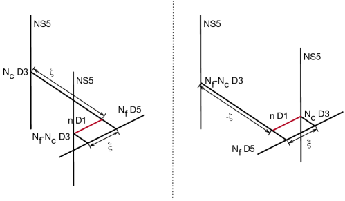
Figure 14: The brane motion representing the Seiberg-like duality of an $\mathcal{N}=4$ SQCD. Vortices are realized as D1-branes denoted by the red line in the figure. The spacetime directions occupied by each brane are summarized in table 6. The distance between two NS5-branes along the 6-direction corresponds to 3d FI parameter $\xi$ while that along the 9-direction corresponds to 1d FI parameter $\zeta$.

Branes	0	1	2	3	4	5	6	7	8	9
NS5	$\times$	$\times$	$\times$	$\times$	$\times$	$\times$
D5	$\times$	$\times$	$\times$				$\times$	$\times$	$\times$
D3	$\times$	$\times$	$\times$							$\times$
D1	$\times$						$\times$

Table 6: The spacetime directions occupied by the branes in figure 14 are marked by $\times$.

The same argument for the previous example suggests that the Seiberg-like duality between the two 3d $\mathcal{N}=4$ theories on D3-branes is equivalent to the wall-crossing of vortex quantum mechanics on D1-branes. In this section, we explicitly realize it by computing the quantum mechanics indices for different 1d FI parameters.

For the 3d $\mathcal{N}=4$ $U(N_{c})$ theory with $N_{f}$ flavors, the moduli space of $n$ vortices is described by the $\mathcal{N}=4$ gauged quantum mechanics illustrated in figure 15, which is a truncation of figure 8.

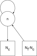
Figure 15: The quiver diagram representation of vortex quantum mechanics for a 3d $\mathcal{N}=4$ SQCD. Each arrow represents the 1d $\mathcal{N}=4$ chiral multiplet. This is a truncation of figure 8.

The refined Witten index of this quantum mechanics is again written as the following JK-residue:

$$I^{n}=\frac{1}{|\mathsf{W}|}\text{JK-Res}_{\eta=\zeta}\left[g^{n}(u)d^{n}u\right]$$ (120)

where $g^{n}(u)$ is now given by

$$g^{n}(u) =\left(\frac{1}{2\sinh\frac{-2\mu}{2}}\right)^{n}\left(\prod_{i\neq j}^{n}\frac{\sinh\frac{u_{i}-u_{j}}{2}}{\sinh\frac{u_{i}-u_{j}-2\mu}{2}}\right)\left(\prod_{i,j=1}^{n}\frac{\sinh\frac{u_{i}-u_{j}-2\mu-2\gamma}{2}}{\sinh\frac{u_{i}-u_{j}-2\gamma}{2}}\right)$$

$$\quad\times\left(\prod_{i=1}^{n}\prod_{b=1}^{N_{c}}\frac{\sinh\frac{u_{i}-m_{b}-2\mu-\gamma}{2}}{\sinh\frac{u_{i}-m_{b}-\gamma}{2}}\right)\left(\prod_{i=1}^{n}\prod_{a=N_{c}+1}^{N_{f}}\frac{\sinh\frac{-u_{i}+m_{a}-2\mu-\gamma}{2}}{\sinh\frac{-u_{i}+m_{a}-\gamma}{2}}\right).$$ (121)

We first compute the quantum mechanics index for $\zeta>0$. The JK-residue rule chooses sets of linearly independent hyperplanes each of which determine $u_{i}$ as follows:

$$u_{i}=\left\{\begin{array}[]{l}u_{j}+2\mu,\\ u_{j}+2\gamma,\\ m_{a}+\gamma,\qquad a\in\{1,\ldots,N_{c}\}.\end{array}\right.$$ (125)

However, a pole intersecting a hyperplane of the first type has the vanishing residue because of zeros of the integrand. Therefore, the contributing poles are written in the following form:

$$u_{i}=m_{a}+(2k_{a}-1)\gamma,\qquad a\in\{1,\ldots,N_{c}\},\quad k_{a}\in\{1,\ldots,n_{a}\}$$ (126)

where $(n_{1},\ldots,n_{N_{c}})$ is a partition of $n$ into $N_{c}$ nonnegative integers. Again every pair $(a,k_{a})$ is assigned to one of $i=1,\ldots,n$ exactly once. Evaluating the JK-residue, we have the following contribution to the index for a given partition $(n_{1},\ldots,n_{N_{c}})$:

$$\left(\prod_{a,b=1}^{N_{c}}\prod_{k_{a}=1}^{n_{a}}\prod_{k_{b}=1}^{n_{b}}\frac{\sinh\frac{m_{a}-m_{b}+2(k_{a}-k_{b})\gamma}{2}}{\sinh\frac{m_{a}-m_{b}-2\mu+2(k_{a}-k_{b})\gamma}{2}}\frac{\sinh\frac{m_{a}-m_{b}-2\mu+2(k_{a}-k_{b}-1)\gamma}{2}}{\sinh\frac{m_{a}-m_{b}+2(k_{a}-k_{b}-1)\gamma}{2}}\right)^{\prime}$$

$$\times\left(\prod_{a=1}^{N_{c}}\prod_{k_{a}=1}^{n_{a}}\prod_{b=1}^{N_{c}}\frac{\sinh\frac{m_{a}-m_{b}-2\mu+2(k_{a}-1)\gamma}{2}}{\sinh\frac{m_{a}-m_{b}+2(k_{a}-1)\gamma}{2}}\right)^{\prime}\left(\prod_{b=1}^{N_{c}}\prod_{k_{b}=1}^{n_{b}}\prod_{a=N_{c}+1}^{N_{f}}\frac{\sinh\frac{-m_{b}+m_{a}-2\mu-2k_{b}\gamma}{2}}{\sinh\frac{-m_{b}+m_{a}-2k_{b}\gamma}{2}}\right).$$ (127)

where ^′ denotes that the vanishing factors are omitted. The Weyl factor $|\mathsf{W}|$ is canceled by factor $n!$ coming from the permutations among $u_{i}$’s. (4.2) is further simplified due to the cancelation between the numerator and the denominator. Summing over all possible partitions of $n$, the index with $\zeta>0$ is given by

$$I^{n}_{\zeta>0}=$$

$$\sum_{\begin{subarray}{c}n_{a}\geq 0,\\ \sum n_{a}=n\end{subarray}}\left(\prod_{a,b=1}^{N_{c}}\prod_{k_{a}=1}^{n_{a}}\frac{\sinh\frac{m_{a}-m_{b}-2\mu+2(k_{a}-n_{b}-1)\gamma}{2}}{\sinh\frac{m_{a}-m_{b}+2(k_{a}-n_{b}-1)\gamma}{2}}\right)\left(\prod_{b=1}^{N_{c}}\prod_{k_{b}=1}^{n_{b}}\prod_{a=N_{c}+1}^{N_{f}}\frac{\sinh\frac{-m_{b}+m_{a}-2\mu-2k_{b}\gamma}{2}}{\sinh\frac{-m_{b}+m_{a}-2k_{b}\gamma}{2}}\right),$$ (128)

which reproduces the vortex partition function of the $\mathcal{N}=4$ $U(N_{c})$ theory with $N_{f}$ flavors on $\mathbb{R}_{\Omega}^{2}\times S^{1}$ Kim:2012uz .

On the other hand, for the index with $\zeta<0$, the JK-residue rule with $\eta=\zeta$ chooses different sets of hyperplanes:

$$u_{i}=\left\{\begin{array}[]{l}u_{j}-2\mu,\\ u_{j}-2\gamma,\\ m_{a}-\gamma,\qquad a\in\{N_{c}+1,\ldots,N_{f}\}.\end{array}\right.$$ (132)

Since a pole intersecting a hyperplane of the first type has the vanishing residue, a relevant pole is written in the following form:

$$u_{i}=m_{a}-(2k_{a}-1)\gamma,\qquad a\in\{N_{c}+1,\ldots,N_{f}\},\quad k_{a}\in\{1,\ldots,n_{a}\}$$ (133)

where $(1,\ldots,n_{a})$ is a partition of $n$ into $N_{f}-N_{c}$ nonnegative integers. The resulting index of vortex quantum mechanics is given by

$$I^{n}_{\zeta<0}=$$

$$\sum_{\begin{subarray}{c}n_{a}\geq 0,\\ \sum n_{a}=n\end{subarray}}\left(\prod_{a,b=N_{c}+1}^{N_{f}}\prod_{k_{b}=1}^{n_{b}}\frac{\sinh\frac{-m_{b}+m_{a}-2\mu+2(k_{b}-n_{a}-1)\gamma}{2}}{\sinh\frac{-m_{b}+m_{a}+2(k_{b}-n_{a}-1)\gamma}{2}}\right)\left(\prod_{a=N_{c}+1}^{N_{f}}\prod_{k_{a}=1}^{n_{a}}\prod_{b=1}^{N_{c}}\frac{\sinh\frac{m_{a}-m_{b}-2\mu-2k_{a}\gamma}{2}}{\sinh\frac{m_{a}-m_{b}-2k_{a}\gamma}{2}}\right).$$ (134)

As expected the index with the negative FI parameter $\zeta<0$ is the vortex partition function of the dual $U(N_{f}-N_{c})$ theory with $N_{f}$ flavors. The sign flip of mass $m_{a}$ is understood because the 3d FI parameter is also flipped under the duality such that the roles of fundamental and anti-fundamental fields are exchanged. This shows that the Seiberg-like duality of a 3d $\mathcal{N}=4$ $U(N_{c})$ theory with fundamental hypers also corresponds to the sign flip of the FI parameter in its vortex quantum mechanics.

The indices in different FI chambers: $\zeta>0$ and $\zeta<0$ do not need to agree due to the non-compact Coulomb branch at $\zeta=0$. Some states can escape through this non-compact branch. One can trace those escaping states by comparing the indices (4.2) and (4.2). Using the same argument for the previous example we show that two indices (4.2) and (4.2) indeed satisfy the following relation:

$$\left(\sum_{m=0}^{\infty}\frac{w^{m}}{m!}\sum_{\cap_{i=1}^{m}H_{i}^{-}\in\text{asymp}^{-}}\mathrm{Res}_{H_{1},\ldots,H_{m}}\left[g^{m}_{-}(u)d^{m}u\right]\right)\left(\sum_{n=0}^{\infty}w^{n}I^{n}_{\zeta>0}\right)$$

$$=\left(\sum_{m=0}^{\infty}\frac{(-w)^{m}}{m!}\sum_{\cap_{i=1}^{m}H_{i}^{+}\in\text{asymp}^{+}}\mathrm{Res}_{H_{1},\ldots,H_{m}}\left[g^{m}_{+}(u)d^{m}u\right]\right)\left(\sum_{n=0}^{\infty}w^{n}I^{n}_{\zeta<0}\right)$$ (135)

where

$$g^{m}_{\pm}(u) =\left(\frac{e^{\pm\frac{1}{2}(2N_{c}-N_{f})(-2\mu)}}{2\sinh\frac{-2\mu}{2}}\right)^{m}\left(\prod_{i\neq j}^{m}\frac{\sinh\frac{u_{i}-u_{j}}{2}}{\sinh\frac{u_{i}-u_{j}-2\mu}{2}}\right)\left(\prod_{i,j=1}^{m}\frac{\sinh\frac{u_{i}-u_{j}-2\mu-2\gamma}{2}}{\sinh\frac{u_{i}-u_{j}-2\gamma}{2}}\right).$$ (136)

Hyperplanes $H_{1}^{\pm},\ldots,H_{m}^{\pm}$ are chosen among

$$u_{i} =\left\{\begin{array}[]{l}\pm\infty,\\ u_{j}\mp 2\mu,\\ u_{j}\mp 2\gamma.\end{array}\right.$$ (140)

Note that $g^{m}_{+}(u)$ and $g^{m}_{-}(u)$ are the same when $N_{f}=2N_{c}$, which is the self-dual case. Therefore, the asymptotic factors in (4.2) cancel each other such that

$$I^{n}_{\zeta>0}=I^{n}_{\zeta<0}$$ (141)

for $N_{f}=2N_{c}$. (141) implies that there is no spectrum jump at $\zeta=0$ when $N_{f}=2N_{c}$. For general $N_{f}\neq 2N_{c}$, one can obtain the nontrivial wall-crossing factor by evaluating the asymptotic residues. However, it turns out that the explicit computations of the asymptotic residues in this example are more complicated than those in the previous example. Instead, it is shown that the explicit form of (4.2) can be obtained by examining large mass limits of the vortex partition functions (4.2) and (4.2) Hwang:2015wna :

$$\sum_{n=0}^{\infty}w^{n}I^{n}_{\zeta>0}=\left(\sum_{n=0}^{\infty}w^{n}I^{n}_{\zeta<0}\right)\left(\prod_{i=1}^{2N_{c}-N_{f}}Z_{\text{hyper}}(x,\tau,w\tau^{2N_{c}-N_{f}-2i+1})\right)$$ (142)

where $\tau=e^{\mu}$ and $x=e^{\gamma}$. $Z_{\text{hyper}}$ is the contribution of a free twisted hypermultiplet, which is given by

$$Z_{\text{hyper}}(x,\tau,w)=\mathrm{PE}\left[\frac{\tau^{-1}w-\tau wx^{2}}{1-x^{2}}\right].$$ (143)

Thus, the wall-crossing factor for the vortex quantum mechanics index corresponds the contribution of the decoupled free twisted hypermultiplets in the dual 3d theory. Indeed, those twisted hypermultiplets describe Coulomb branches of the 3d theory Gaiotto:2008ak ; Kim:2012uz ; Yaakov:2013fza ; Gaiotto:2013bwa . Again we observe that the wall-crossing of vortex quantum mechanics captures the information of Coulomb branch of the 3d theory.

We have proven that the vortex quantum mechanics indices in different FI chambers: $\zeta>0$ and $\zeta<0$ exactly reproduce the vortex partition functions of a 3d $\mathcal{N}=4$ Seiberg-like dual pair. This shows that under the Seiberg-like duality, vortex quantum mechanics for a 3d $\mathcal{N}=4$ SQCD experiences the wall-crossing controlled by FI parameter $\zeta$. Furthermore, from the identity (142), we show that the BPS index of the escaping states at the wall $\zeta=0$ is given by

$$Z^{\text{wall}} =\prod_{i=1}^{2N_{c}-N_{f}}Z_{\text{hyper}}(x,\tau,w\tau^{2N_{c}-N_{f}-2i+1})$$ (144)

$$=\mathrm{PE}\left[\frac{\sinh\left[(2N-M)\mu\right]\sinh(\mu+\gamma)}{\sinh\mu\sinh\gamma}w\right],$$ (145)

which is also identified as the index of the 3d twisted hypermultiplets describing Coulomb branches of the moduli space.

4.3 Linear quiver examples

4.3.1 $T_{\rho}[SU(N)]$

We have seen that for a 3d SQCD, the Seiberg-like duality is equivalent to the wall-crossing of vortex quantum mechanics controlled by the 1d FI parameter $\zeta$. In this section, we would like to ask whether this phenomenon can be generalized to more complicated cases such as linear quiver gauge theories we examined in section 3. We will see that even in such cases, the equivalence between the 3d Seiberg-like duality and the wall-crossing of vortex quantum mechanics is observed.

First let us consider $T_{\rho}[SU(N)]$ theories. The vortex partition functions of $T_{\rho}[SU(N)]$ theories are given by (3.1). We should remind you that this result is for positive 3d FI parameters $\xi_{1},\ldots,\xi_{L}>0$. In order to examine the Seiberg-like dualities of $T_{\rho}[SU(N)]$ theories, however, we have to relax this positive FI condition because the Seiberg-like dualities incorporate nontrivial FI mappings. For concreteness, let us consider $T_{[N_{1},N_{2}-N_{1},N_{3}-N_{2}]}[SU(N_{3})]$ having two gauge nodes. We have a duality chain including this theory as shown in figure 16.

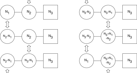
Figure 16: The Seiberg-like duality chain of $T_{[N_{1},N_{2}-N_{1},N_{3}-N_{2}]}[SU(N_{3})]$.

The duality chain contains all possible ranges of the FI parameters. If we assume $\xi^{\mathbf{1}}_{1}=\xi_{1}>0$ and $\xi^{\mathbf{1}}_{2}=\xi_{2}>0$, each theory in the duality chain has the FI parameters in the following ranges:

$$\begin{array}[]{lccclcc}\xi^{\mathbf{1}}_{1}=\xi_{1}&>&0,&&\xi^{\mathbf{1}}_{2}=\xi_{2}&>&0,\\ \xi^{\mathbf{2}}_{1}=-\xi_{1}&<&0,&&\xi^{\mathbf{2}}_{2}=\xi_{1}+\xi_{2}&>&|\xi^{\mathbf{2}}_{1}|,\\ \xi^{\mathbf{3}}_{1}=\xi_{2}&>&0,&&\xi^{\mathbf{3}}_{2}=-\xi_{1}-\xi_{2}&<&-|\xi^{\mathbf{3}}_{1}|,\\ \xi^{\mathbf{4}}_{1}=-\xi_{2}&<&0,&&\xi^{\mathbf{4}}_{2}=-\xi_{1}&<&0,\\ \xi^{\mathbf{5}}_{1}=-\xi_{1}-\xi_{2}&<&-|\xi^{\mathbf{5}}_{2}|,&&\xi^{\mathbf{5}}_{2}=\xi_{1}&>&0,\\ \xi^{\mathbf{6}}_{1}=\xi_{1}+\xi_{2}&>&|\xi^{\mathbf{6}}_{2}|,&&\xi^{\mathbf{6}}_{2}=-\xi_{2}&<&0\\ \end{array}$$ (152)

where $\xi^{\mathbf{k}}_{l}$ is an FI parameter of the $\mathbf{k}$-th theory in the duality chain. These FI mappings under the Seiberg-like dualities can be read off from the brane setup, figure 17.

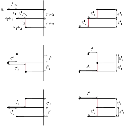
Figure 17: The brane setups representing the duality chain in figure 16 are shown. NS5-branes, D5-branes, D3-branes, D1-branes are denoted by black dots, black vertical lines, black horizontal lines and red vertical lines respectively. The vertical distances between NS5-branes correspond to 3d FI parameters $\xi_{l}$ while the horizontal distances between NS5-branes correspond to 1d FI parameters $\zeta_{l}$.

To the best of our knowledge, the vortex partition functions of $T_{\rho}[SU(N)]$ with general FI parameter ranges have not been investigated in the literatures. For this reason, so far it is not manifest to study the Seiberg-like duality of $T_{\rho}[SU(N)]$ using the vortex partition function.

On the other hand, we have seen that two vortex quantum mechanics for a 3d Seiberg-like dual pair are related by a change of 1d FI parameters, at least for SQCDs. In other words, the two vortex quantum mechanics should be the same except the FI parameters. We claim that this relation still holds for more complicated theories such as $T_{\rho}[SU(N)]$ we are now considering. For example, the first theory in the duality chain has vortex quantum mechanics described in figure 18.

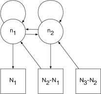
Figure 18: Vortex quantum mechanics for $T_{[N_{1},N_{2}-N_{1},N_{3}-N_{2}]}[SU(N_{3})]$.

The vortex quantum mechanics has positive FI parameters, $\zeta^{\mathbf{1}}_{1}>0$ and $\zeta^{\mathbf{1}}_{2}>0$. The second theory in the duality chain then should have the same vortex quantum mechanics except FI parameters, which are now in different ranges: $\zeta^{\mathbf{2}}_{1}<0$ and $\zeta^{\mathbf{2}}_{2}>|\zeta^{\mathbf{2}}_{1}|$. Indeed, we claim that all those six theories in the 3d duality chain have the same vortex quantum mechanics with different 1d FI parameters in the following ranges:

$$\begin{array}[]{ccccccc}\zeta^{\mathbf{1}}_{1}&>&0,&&\zeta^{\mathbf{1}}_{2}&>&0,\\ \zeta^{\mathbf{2}}_{1}&<&0,&&\zeta^{\mathbf{2}}_{2}&>&|\zeta^{\mathbf{2}}_{1}|,\\ \zeta^{\mathbf{3}}_{1}&<&-|\zeta^{\mathbf{3}}_{2}|,&&\zeta^{\mathbf{3}}_{2}&>&0,\\ \zeta^{\mathbf{4}}_{1}&<&0,&&\zeta^{\mathbf{4}}_{2}&<&0,\\ \zeta^{\mathbf{5}}_{1}&>&0,&&\zeta^{\mathbf{5}}_{2}&<&-|\zeta^{\mathbf{5}}_{1}|,\\ \zeta^{\mathbf{6}}_{1}&>&|\zeta^{\mathbf{6}}_{2}|,&&\zeta^{\mathbf{6}}_{2}&<&0\end{array}$$ (159)

where $\zeta^{\mathbf{k}}_{l}$ is an FI parameter of vortex quantum mechanics for the $\mathbf{k}$-th theory in the duality chain. An interesting thing is that the number of phases of the 3d duality chain and that of 1d FI parameters are the same. This is a clue that the 3d Seiberg-like duality and the wall-crossing of vortex quantum mechanics are related.

One should note that quantum mechanics in figure 18 with the FI parameters (159) is exactly the world-volume theory of D1-branes in figure 17. The Seiberg-like duality of $T_{\rho}[SU(N)]$ and the wall-crossing of its vortex quantum mechanics are inferred from the same brane motion. Thus, we expect that the quantum mechanics with the FI parameters (159) correctly describes the vortex moduli spaces of the 3d theories in the duality chain.

Furthermore, we provide additional evidence by explicitly computing the quantum mechanics indices for different FI parameters. In the previous section, we have seen that the vortex partition functions of an $\mathcal{N}=4$ SQCD dual pair agree up to the contribution of decoupled twisted hypermultiplets. The number of the decoupled twisted hypermultiplets is determined by the rank difference between the gauge groups of the dual pair. This is a consequence of the fact that a dual pair must have the same number of Coulomb branches, which is determined by the gauge group rank Gaiotto:2008ak ; Kim:2012uz ; Yaakov:2013fza ; Gaiotto:2013bwa . This is still true for $T_{\rho}[SU(N)]$ theories. Indeed, we have checked that the following relations hold among the six quantum mechanics indices in different FI chambers:

$$\begin{aligned} Z_{\mathbf{1}}/Z_{\mathbf{2}}&=Z^{\text{wall}}_{N_{1},N_{2}}(w_{1}),\\ Z_{\mathbf{2}}/Z_{\mathbf{3}}&=Z^{\text{wall}}_{N_{2},N_{3}+N_{2}-N_{1}}(w_{1}w_{2}),\\ Z_{\mathbf{3}}/Z_{\mathbf{4}}&=Z^{\text{wall}}_{N_{2}-N_{1},N_{3}-N_{1}}(w_{2}),\\ Z_{\mathbf{4}}/Z_{\mathbf{5}}&=Z^{\text{wall}}_{N_{3}-N_{1},2N_{3}-N_{2}}(w_{1}),\\ Z_{\mathbf{5}}/Z_{\mathbf{6}}&=Z^{\text{wall}}_{N_{3}-N_{2},N_{3}-N_{2}+N_{1}}(w_{1}w_{2}),\\ Z_{\mathbf{6}}/Z_{\mathbf{1}}&=Z^{\text{wall}}_{N_{3}-N_{2}+N_{1},N_{1}+N_{3}}(w_{2})\end{aligned}$$ (160)

where $Z_{\mathbf{k}}$ on the left hand side is the generating function of the vortex indices in the $\mathbf{k}$-th FI chamber:

$$Z_{\mathbf{k}}=\sum_{n_{1}=0}^{\infty}\sum_{n_{2}=0}^{\infty}w_{1}^{n_{1}}w_{2}^{n_{2}}I_{\mathbf{k}}^{n_{1},n_{2}}$$ (161)

while $Z^{\text{wall}}_{N,M}$ on the right hand side is the wall-crossing factor:

$$Z^{\text{wall}}_{N,M}(w)=\mathrm{PE}\left[\frac{\sinh\left[(2N-M)\mu\right]\sinh(\mu+\gamma)}{\sinh\mu\sinh\gamma}w\right].$$ (162)

Here we allow negative $2N-M$ as well such that

$$Z^{\text{wall}}_{N,M}(w)=Z^{\text{wall}}_{M-N,M}(w)^{-1}$$ (163)

for $2N-M<0$. (145) tells us that $Z^{\text{wall}}_{N,M}$ with $2N\geq M$ is exactly the contribution of $2N-M$ decoupled twisted hypermultiplets. Thus, the wall-crossing factors in (160) reflect the correct number of decoupled twisted hypermultiplets at each duality step. Although we have examined a two gauge node example, this behavior of the quantum mechanics index is expected for the other $T_{\rho}[SU(N)]$ theories as well. Therefore, we expect that the Seiberg-like duality of general $T_{\rho}[SU(N)]$ is equivalent to the wall-crossing of its vortex quantum mechanics.

4.3.2 $\mathcal{N}=2$ linear quiver examples

Next let us consider $\mathcal{N}=2$ linear quiver examples, which we have examined in section 3.2. We illustrate some examples that exhibit the equivalence of the 3d Seiberg-like duality and the wall-crossing of vortex quantum mechanics. The relation between the Seiberg-like duality and the vortex wall-crossing for general $\mathcal{N}=2$ theories will be worth studying, which we relegate to future work.

The examples we are considering in this section have a duality chain illustrated in figure 19.

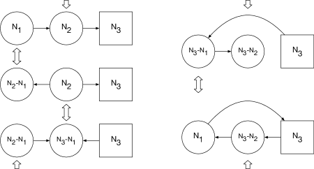
Figure 19: A typical duality chain of an $\mathcal{N}=2$ linear quiver theory we are considering. Unlike $T_{\rho}[SU(N)]$, an arrow has a direction which can be flipped under the duality. In addition, a new arrow can appear after the duality action.

The corresponding vortex quantum mechanics is given by figure 11 with $L=2$. One should note that, unlike the previous $T_{\rho}[SU(N)]$ example, vortex quantum mechanics now has only five FI chambers instead of six:

$$\begin{array}[]{ccccccc}\zeta^{\mathbf{1}}_{1}&>&0,&&\zeta^{\mathbf{1}}_{2}&>&0,\\ \zeta^{\mathbf{2}}_{1}&<&0,&&\zeta^{\mathbf{2}}_{2}&>&|\zeta^{\mathbf{2}}_{1}|,\\ \zeta^{\mathbf{3}}_{1}&<&-|\zeta^{\mathbf{3}}_{2}|,&&\zeta^{\mathbf{3}}_{2}&>&0,\\ \zeta^{\mathbf{4}}_{1}&<&0,&&\zeta^{\mathbf{4}}_{2}&<&0,\\ \zeta^{\mathbf{5}}_{1}&>&0,&&\zeta^{\mathbf{5}}_{2}&<&0.\end{array}$$ (169)

The fifth chamber was divided into two chambers: $|\zeta^{\mathbf{5}}_{1}|<|\zeta^{\mathbf{5}}_{2}|$ and $|\zeta^{\mathbf{5}}_{1}|>|\zeta^{\mathbf{5}}_{2}|$ for $T_{\rho}[SU(N)]$ while it is not for the current example. This is because there is only one bi-fundamental chiral multiplet between adjacent gauge nodes of vortex quantum mechanics. Indeed, the duality chain in figure 19 also includes only five theories instead of six. This is the first clue that the 3d Seiberg-like duality relates to the wall-crossing of vortex quantum mechanics for $\mathcal{N}=2$ linear quiver theories as well.

The simplest example is an $(N,N,N)$-type quiver theory. The theory has gauge group $U(N)\times U(N)$ and flavor group $U(N)$. We introduce the CS interaction for each gauge node as well as the BF interaction between the $U(1)$ parts of them. The level of those CS and BF interactions are chosen as follows:

$$\begin{gathered}\kappa^{(1)}=\frac{N}{2},\qquad\kappa^{(2)}=0,\\ \Delta\kappa_{U(1)}^{(1)}=0,\qquad\Delta\kappa_{U(1)}^{(2)}=1,\\ \kappa_{U(1)}^{(1,2)}=-\frac{1}{2}\end{gathered}$$ (173)

where $\kappa^{(l)}$ is the $U(N)$ CS level while $\Delta\kappa_{U(1)}^{(l)}$ is the additional CS level shift for the $U(1)$ part of $U(N)$. $k_{U(1)}^{(l,l+1)}$ is the BF level. Those ranks of the nodes and CS/BF levels are chosen such that the theory has simple Seiberg-like duals as we explain shortly. Vortex quantum mechanics for this theory is described in figure 20 with the Wilson lines (55).

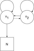
Figure 20: Vortex quantum mechanics for a $(N,N,N)$-type quiver theory is illustrated. If the parent 3d theory has CS/BF interactions, the quantum mechanics also has the corresponding Wilson lines shown in (55).

We illustrate the duality chain of this theory in figure 21, which is a special case of figure 19.

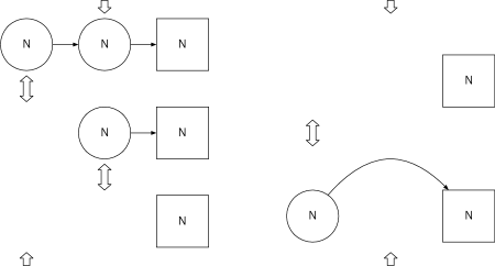
Figure 21: The Seiberg-like duality chain of a $(N,N,N)$-type quiver theory is represented. This is a special case of figure 19. Since every node has the same rank, a node to which the duality action is applied disappears after the duality action. Each theory may have nontrivial CS/BF interactions, which is explained in the paragraph before (208).

The duality chain is basically obtained by the rule examined in Aharony:1997gp ; Benini:2011mf with some additional ingredients regarding $U(1)$ factors. The first dual theory, i.e., the second theory in the duality chain, can be obtained by taking the duality action on the leftmost node. Following the duality rule in Aharony:1997gp ; Benini:2011mf , the dual gauge rank is given by $N-N=0$; i.e, the first node should vanish. Since the number of fundamental chiral multiplets charged under the first gauge node is equal to the twice of the CS level of that node, we expect that an extra decoupled chiral multiplet appears in the dual theory as it happens in a single gauge node case. This extra chiral multiplet corresponds to a gauge invariant monopole operator in the original theory, which describes a Coulomb branch of the moduli space. Furthermore, the duality action also has a nontrivial effect on the CS level of the second node. In Benini:2011mf , it is argued that the CS level of the second node is shifted by the amount of the CS level of the first node and becomes $\frac{N}{2}$.

On the other hand, the duality effect related to the BF interaction has not been discussed in the literatures. Here we trace this effect of the BF interaction by examining the Abelian example: the $(1,1,1)$ theory and its dual theory. The theory has the CS and BF interactions of the levels in (173). Since there is no distinction between the $U(N)$ CS level and the $U(1)$ CS level for $N=1$, each gauge node just has the CS interaction of level $\kappa_{l}\equiv\kappa^{(l)}+\Delta\kappa_{U(1)}^{(l)}$. Without the BF interaction, the rule in Benini:2011mf tells us that the dual theory has CS level $\kappa_{1}+\kappa_{2}=\frac{3}{2}$. However, the level half BF interaction is not avoidable due to the regularization of the fermion in the bi-fundamental chiral multiplet. Indeed, we will see that if the BF interaction of level $-\frac{1}{2}$ is included, the dual theory has CS level $\frac{1}{2}$ rather than $\frac{3}{2}$.

In order to see this effect, let us first analyze the vacuum moduli space of the $(1,1,1)$ theory. In section 2.1, we have reviewed that a 3d $\mathcal{N}=2$ $U(1)$ theory has three types of vacua: Coulomb, Higgs and topological vacuum, For general gauge groups, vacua of mixed types are also available. The vacuum equations are given by

$$\sum_{i}2\pi n^{(l)}_{i}|Q_{i}|^{2}-F^{(l)}(\sigma)=0,$$ (175)

$$m_{i}(\sigma)^{2}|Q_{i}|^{2}=0$$ (176)

where $l$ labels each $U(1)$ gauge node and $i$ labels each charged chiral multiplet. $F^{(l)}(\sigma)\equiv\xi_{\text{eff}}+\kappa_{\text{eff}}\sigma$ is given by equation (11). For the $(1,1,1)$ theory,

$$F^{(1)}(\sigma) =\xi_{1}+\frac{1}{2}\sigma_{1}-\frac{1}{2}\sigma_{2}+\frac{1}{2}|\sigma_{1}-\sigma_{2}|,$$ (177)

$$F^{(2)}(\sigma) =\xi_{2}+\sigma_{2}-\frac{1}{2}\sigma_{1}+\frac{1}{2}|\sigma_{2}|-\frac{1}{2}|\sigma_{1}-\sigma_{2}|$$ (178)

where the contribution of the BF interaction is taken into account. For $\xi_{l}>0$, $F^{(1)}(\sigma)$ is always positive. Therefore, $m_{12}(\sigma)=\sigma_{1}-\sigma_{2}$, mass of bi-fundamental $Q_{12}$, should vanish so that $Q_{12}$ can have the nonzero vacuum expectation value. Then $F^{(2)}(\sigma)$ is also positive such that the theory only has a Higgs vacuum at $\sigma_{1}=\sigma_{2}=0$. $Q_{12}$ and $Q_{23}$ are determined by

$$\begin{gathered}|Q_{12}|^{2}-\frac{\xi_{1}}{2\pi}=0,\\ |Q_{23}|^{2}-|Q_{12}|^{2}-\frac{\xi_{2}}{2\pi}=0.\end{gathered}$$ (181)

Thus, the vacuum moduli space of the theory is $\mathbb{C}P^{0}$. If either $\xi_{1}$ or $\xi_{1}+\xi_{2}$ vanishes, new Coulomb vacua appear. They are parameterized by $\sigma_{1}^{\prime}\equiv\sigma_{1}-\sigma_{2}\leq 0$ or $\sigma_{2}\leq 0$ respectively. This is consistent with the duality chain in figure 21. In the third theory, for example, those two Coulomb branches are described by two chiral multiplets of masses $\xi_{1}$ and $\xi_{1}+\xi_{2}$.

Now let us ask what the correct CS level of the dual theory is. The answer is more clear if we allow a generic value for the second CS level of the original theory. For later use, we also attach more flavors; i.e., we increase the rank of the last flavor node. With CS level $\kappa$ of the second node and rank $N$ of the last node, $F^{(l)}(\sigma)$’s for the original theory are rewritten in the following way:

$$F^{(1)}(\sigma) =\xi_{1}+\frac{1}{2}\sigma_{1}-\frac{1}{2}\sigma_{2}+\frac{1}{2}|\sigma_{1}-\sigma_{2}|,$$ (182)

$$F^{(2)}(\sigma) =\xi_{2}+\kappa\sigma_{2}-\frac{1}{2}\sigma_{1}+\frac{N}{2}|\sigma_{2}|-\frac{1}{2}|\sigma_{1}-\sigma_{2}|.$$ (183)

Assuming $\xi_{l}>0$, $F^{(1)}(\sigma)$ is always positive as before. Thus, the first gauge node only allows a Higgs vacuum solution. We ask whether there exists a Coulomb or topological vacuum solution for the second node, which satisfies $F^{(2)}(\sigma)=0$. Since the first gauge node has a Higgs vacuum solution, $\sigma_{1}-\sigma_{2}$ should vanish. $F^{(2)}(\sigma)$ is then written as follows:

$$F^{(2)}(\sigma) =\xi_{2}+\kappa\sigma_{2}-\frac{1}{2}\sigma_{2}+\frac{N}{2}|\sigma_{2}|$$ (184)

such that $F^{(2)}(\sigma)=0$ has a topological vacuum solution:

$$\sigma_{2}=\left\{\begin{array}[]{cc}-\frac{\xi_{2}}{\kappa+\frac{N-1}{2}},&\kappa<-\frac{N-1}{2},\\ -\frac{\xi_{2}}{\kappa-\frac{N+1}{2}},&\kappa>\frac{N+1}{2}.\end{array}\right.$$ (187)

Therefore, the theory has a Higgs-topological vacuum if $\kappa<-\frac{N-1}{2}$ or $\kappa>\frac{N+1}{2}$. As noted in section 2.1 the effective theory at this classical vacuum is the $\mathcal{N}=2$ $U(1)_{\kappa_{\text{eff}}}$ CS theory where $\kappa_{\text{eff}}=\kappa+\frac{N-1}{2}$ for $\kappa<-\frac{N-1}{2}$ or $\kappa_{\text{eff}}=\kappa-\frac{N+1}{2}$ for $\kappa>\frac{N+1}{2}$. Thus, the actual number of quantum topological vacua is $|\kappa_{\text{eff}}|$. In addition, there is Higgs-Higgs vacua at $\sigma_{1}=\sigma_{2}=0$ regardless of the value of $\kappa$, which are determined by

$$\begin{gathered}|Q_{12}|^{2}-\frac{\xi_{1}}{2\pi}=0,\\ \sum_{a=1}^{N}|Q_{23,a}|^{2}-|Q_{12}|^{2}-\frac{\xi_{2}}{2\pi}=0.\end{gathered}$$ (190)

This defines the Higgs branch of the moduli space, which is given by $\mathbb{C}P^{N-1}$. This splits into $N$ separate vacua if we turn on small real masses for $Q_{23,a}$’s. As a result, the number of vacua, or the Witten index, of the theory is given by

$$I=\left\{\begin{array}[]{cc}-\kappa+\frac{1}{2}N+\frac{1}{2},&\kappa<-\frac{N-1}{2},\\ N,&-\frac{N-1}{2}\leq\kappa\leq\frac{N+1}{2},\\ \kappa+\frac{1}{2}N-\frac{1}{2},&\frac{N+1}{2}<\kappa.\end{array}\right.$$ (194)

When an FI parameter is turned off, we also have Coulomb vacua. If $\xi_{1}=0$, there is a Coulomb branch of the moduli space parameterized by $\sigma_{1}^{\prime}=\sigma_{1}-\sigma_{2}\leq 0$. If $\xi_{1}+\xi_{2}=0$ and $\kappa=\frac{N+1}{2}$, there is another Coulomb branch parameterized by $\sigma_{2}\leq 0$; if we choose $\kappa=-\frac{N-1}{2}$, the second Coulomb branch is parameterized by positive $\sigma_{2}\geq 0$.

Taking the duality action on the first node, the dual theory is given by the $U(1)_{\kappa^{\prime}}$ theory with $N$ fundamental chiral multiplets. We want to determine CS level $\kappa^{\prime}$ that gives the same Witten index as the original theory. First note that $F(\sigma)$ for the dual theory is given by

$$F(\sigma)=\xi_{2}+\kappa^{\prime}\sigma+\frac{N}{2}|\sigma|.$$ (195)

Depending on the value of $\kappa^{\prime}$, $F(\sigma)=0$ allows the following solution:

$$\sigma=\left\{\begin{array}[]{cc}-\frac{\xi_{2}}{\kappa^{\prime}+\frac{N}{2}},&\kappa^{\prime}<-\frac{N}{2},\\ -\frac{\xi_{2}}{\kappa^{\prime}-\frac{N}{2}},&\kappa^{\prime}>\frac{N}{2},\end{array}\right.$$ (198)

which has topological multiplicity $-\kappa^{\prime}-\frac{N}{2}$ or $\kappa^{\prime}-\frac{N}{2}$ respectively. Taking Higgs vacua into account, the Witten index of the dual theory is given by

$$I=\left\{\begin{array}[]{cc}-\kappa^{\prime}+\frac{1}{2}N,&\kappa^{\prime}<-\frac{N}{2},\\ N,&-\frac{N}{2}\leq\kappa^{\prime}\leq\frac{N}{2},\\ \kappa^{\prime}+\frac{1}{2}N,&\frac{N}{2}<\kappa^{\prime}.\end{array}\right.$$ (202)

Thus, the dual theory must have CS level $\kappa^{\prime}=\kappa-\frac{1}{2}$ in order to have the same Witten index as the original theory. This is different from the duality rule in Benini:2011mf , $\kappa^{\prime}=\kappa+\frac{1}{2}$, where the shift by $\frac{1}{2}$ is the result of the CS interaction of the first node. Here we see that there is an additional shift by $-1$, which should be the result of the BF interaction of level $-\frac{1}{2}$.

In general we expect that our level half BF interaction yields another CS level shift for the second gauge node, but only for the $U(1)$ part because the BF interaction is only relevant for the $U(1)$ parts of the gauge nodes. It turns out that this expectation is consistent with what we observe from the vortex partition function analysis. Thus, adopting this additional shift due to the presence of the BF interaction, the CS level for the $U(1)$ part of the second node is shifted by $-1$ after the duality action. This is why we have engineered the original $(N,N,N)$ theory to have the CS/BF levels as in (173), especially $\Delta\kappa_{U(1)}^{(2)}=1$. The second theory in the duality chain is then the $U(N)_{\frac{N}{2}}$ theory without the additional CS level shift for the $U(1)$ part. The theory also contains $N$ fundamental chiral multiplets and one decoupled chiral multiplet. The gauge theory sector is a familiar SQCD. We know that this theory is dual to a single chiral multiplet. Thus, the next dual theory, the third theory in the duality chain, is a theory of two chiral multiplets. These two chiral multiplets describe the two Coulomb branches of the moduli space, which we have observed in the vacuum analysis. The fifth and fourth theories can be obtained by sequentially taking the duality actions on the second node and the first node of the original theory. They are also given by the $U(N)_{\frac{N}{2}}$ theory and the two-chiral theory. Those five theories in the duality chain have the following FI parameters:

$$\begin{array}[]{lll}\xi^{\mathbf{1}}_{1}=\xi_{1},&&\xi^{\mathbf{1}}_{2}=\xi_{2},\\ \xi^{\mathbf{2}}_{1}=\varnothing,&&\xi^{\mathbf{2}}_{2}=\xi_{1}+\xi_{2},\\ \xi^{\mathbf{3}}_{1}=\varnothing,&&\xi^{\mathbf{3}}_{2}=\varnothing,\\ \xi^{\mathbf{4}}_{1}=\varnothing,&&\xi^{\mathbf{4}}_{2}=\varnothing,\\ \xi^{\mathbf{5}}_{1}=\xi_{1},&&\xi^{\mathbf{5}}_{2}=\varnothing\end{array}$$ (208)

where $\varnothing$ means that the corresponding gauge node vanishes. We assume $\xi_{1},\xi_{2}>0$.

We also comment that if the 3d gauge group is Abelian, our construction of vortex quantum mechanics has ambiguity for the Wilson line part, which reflects the 3d CS action. For the Abelian 3d gauge group, there is no distinction between $\kappa^{(l)}$ and $\Delta\kappa_{U(1)}^{(l)}$. However, their counterparts in vortex quantum mechanics are distinguished. One is realized as a gauge Wilson line while the other is realized as a global Wilson line. Even though both constructions of vortex quantum mechanics give the same vortex partition function, their wall-crossing behaviors are completely different. We propose that this ambiguity can be resolved by demanding the wall-crossing behavior compatible with the 3d Seiberg-like duality. For the Abelian $(1,1,1)$ theory, we follow the prescription that the assignment of CS levels for non-Abelian gauge groups (173) still holds for the Abelian gauge group. Then, as we will see, the proposed construction of vortex quantum mechanics for the $(1,1,1)$ theory shows claimed wall-crossing behavior compatible with the 3d Seiberg-like duality.

Now let us move on to the vortex partition functions. Recall that vortex quantum mechanics for the $(N,N,N)$ theory is given by figure 20. We propose that the other theories in the duality chain share the same vortex quantum mechanics with different 1d FI parameters shown in (169). Using the JK-residue formula (25), one can obtain the index of vortex quantum mechanics in each FI chamber. The results are organized as follows:

$$\begin{aligned} Z_{\mathbf{1}}&=\sum_{n_{1}}^{\infty}\sum_{n_{2}=0}^{\infty}(-w_{1})^{n_{1}}w_{2}^{n_{2}}I^{n_{1},n_{2}}_{\mathbf{1}}=\mathrm{PE}\left[-\frac{x^{\frac{N}{2}+1}w_{1}}{1-x^{2}}-\frac{x^{\frac{N}{2}+1}\tau^{\frac{N}{2}}w_{1}w_{2}}{1-x^{2}}\right],\\ Z_{\mathbf{2}}&=\sum_{n_{1}}^{\infty}\sum_{n_{2}=0}^{\infty}(-w_{1})^{n_{1}}w_{2}^{n_{2}}I^{n_{1},n_{2}}_{\mathbf{2}}=\mathrm{PE}\left[-\frac{x^{\frac{N}{2}+1}\tau^{\frac{N}{2}}w_{1}w_{2}}{1-x^{2}}\right],\\ Z_{\mathbf{3}}&=\sum_{n_{1}}^{\infty}\sum_{n_{2}=0}^{\infty}(-w_{1})^{n_{1}}w_{2}^{n_{2}}I^{n_{1},n_{2}}_{\mathbf{3}}=1,\\ Z_{\mathbf{4}}&=\sum_{n_{1}}^{\infty}\sum_{n_{2}=0}^{\infty}(-w_{1})^{n_{1}}w_{2}^{n_{2}}I^{n_{1},n_{2}}_{\mathbf{4}}=1,\\ Z_{\mathbf{5}}&=\sum_{n_{1}}^{\infty}\sum_{n_{2}=0}^{\infty}(-w_{1})^{n_{1}}w_{2}^{n_{2}}I^{n_{1},n_{2}}_{\mathbf{1}}=\mathrm{PE}\left[-\frac{x^{\frac{N}{2}+1}w_{1}}{1-x^{2}}\right]\end{aligned}$$ (209)

where we have introduced the additional negative sign to vorticity fugacity $w_{1}$ to simplify the expressions. We have numerically checked (209) up to $n_{1},n_{2}\leq 3$ for $N=1,2,3$.

Since the theories in the duality chain except the first one have a single or no gauge node, we already know their vortex partition functions. The quantum mechanics indices (209) in different FI chambers correctly reproduce them. Furthermore, the wall-crossing factors, which are given by the ratios of two indices in adjacent FI chambers, are exactly the contributions of the gauge singlet chiral multiplets appearing after the duality actions. Thus, the $(N,N,N)$ theory is the first example showing that the proposed equivalence between the 3d Seiberg-like duality and the wall-crossing of vortex quantum mechanics can be generalized to an $\mathcal{N}=2$ linear quiver gauge theory.

Our next example is a $(1,1,N)$-type quiver theory. The $(N,N,N)$ theory we have considered so far flows to a free theory of two chiral multiplets in the IR limit. The $(1,1,N)$ theory, on the other hand, flows to an interacting IR fixed point. This example shows that the equivalence between the 3d Seiberg-like duality and the vortex wall-crossing can be generalized to an $\mathcal{N}=2$ linear quiver theory flowing to an interacting IR fixed point.

The duality chain containing the $(1,1,N)$ theory is shown in figure 22.

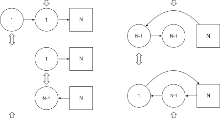
Figure 22: The Seiberg-like duality chain of a $(1,1,N)$-type quiver theory is represented. Note that in the third duality action, the roles of the first node and the second node are exchanged.

The CS/BF levels of the first theory are chosen as follows:

$$\begin{gathered}\kappa^{(1)}=\frac{1}{2},\qquad\kappa^{(2)}=\frac{N-1}{2},\\ \Delta\kappa_{U(1)}^{(1)}=0,\qquad\Delta\kappa_{U(1)}^{(2)}=1,\\ \kappa_{U(1)}^{(1,2)}=-\frac{1}{2}\end{gathered}$$ (213)

so that the second theory is given by the $U(1)_{\frac{N}{2}}$ theory with $N$ fundamental chiral multiplets and one decoupled chiral multiplet $V_{1-}$. Again this is a familiar SQCD, but now it flows to an interacting IR fixed point. Its Seiberg-like (or Aharony) dual theory is given by the $U(N-1)_{-\frac{N}{2}}$ theory with $N$ anti-fundamental chiral multiplets and two gauge singlet chiral multiplets $V_{1-}$ and $V_{2-}$. $V_{1-}$ is from the first duality action and $V_{2-}$ is from the second duality action. $V_{2-}$ couples to the gauge theory via the following superpotential Aharony:1997gp ; Benini:2011mf :

$$W=V_{2-}v_{+}$$ (214)

where $v_{+}$ is the gauge invariant monopole operator of the $U(N-1)_{-\frac{N}{2}}$ theory. Both $V_{1-}$ and $V_{2-}$ describe the Coulomb branches of the moduli space while $v_{+}$ is lifted by the superpotential (214). The fifth and fourth theories are obtained by taking the duality actions on the second node and the first node of the first theory sequentially. The FI parameters of those five theories in the duality chain are as follows:

$$\begin{array}[]{lll}\xi^{\mathbf{1}}_{1}=\xi_{1},&&\xi^{\mathbf{1}}_{2}=\xi_{2},\\ \xi^{\mathbf{2}}_{1}=\varnothing,&&\xi^{\mathbf{2}}_{2}=\xi_{1}+\xi_{2},\\ \xi^{\mathbf{3}}_{1}=\varnothing,&&\xi^{\mathbf{3}}_{2}=-\xi_{1}-\xi_{2},\\ \xi^{\mathbf{4}}_{1}=-\xi_{1},&&\xi^{\mathbf{4}}_{2}=-\xi_{2},\\ \xi^{\mathbf{5}}_{1}=\xi_{1},&&\xi^{\mathbf{5}}_{2}=-\xi_{2}.\end{array}$$ (220)

From the result of section 3.2, vortex quantum mechanics for the $(1,1,N)$ theory is represented by the quiver diagram shown in figure 23.

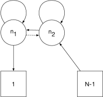
Figure 23: Vortex quantum mechanics for a $(1,1,N)$-type quiver theory is illustrated. If the parent 3d theory has CS/BF interactions, the quantum mechanics also has the corresponding Wilson lines shown in (55).

The index in each FI chamber can be computed using the JK-residue formula (25). One should note that, except the fifth theory, the theories in the duality chain are equivalent to linear quiver gauge theories with positive FI parameters up to charge conjugation. We already know the vortex partition functions of those types of theories from (3.2) using charge conjugation. Indeed, we have confirmed that the index in each FI chamber of quantum mechanics in figure 23 correctly reproduces the vortex partition function from (3.2) except the fifth theory, for which we don’t have other independent computations of the vortex partition function.

Since those four vortex partition functions are now more complicated, we don’t explicitly write them down here. Nevertheless, the wall-crossing factors given by the ratios of two indices in adjacent FI chambers are still written in terms of simple Plethystic exponentials:

$$\begin{aligned} Z^{\text{wall}}_{1}&=Z_{\mathbf{1}}/Z_{\mathbf{2}}=\mathrm{PE}\left[-\frac{x^{\frac{3}{2}}w_{1}}{1-x^{2}}\right],\\ Z^{\text{wall}}_{2}&=Z_{\mathbf{2}}/Z_{\mathbf{3}}=\mathrm{PE}\left[-\frac{x^{2-\frac{N}{2}}\tau^{\frac{N}{2}}w_{1}w_{2}}{1-x^{2}}\right],\\ Z^{\text{wall}}_{3}&=Z_{\mathbf{3}}/Z_{\mathbf{4}}=\mathrm{PE}\left[\frac{x^{\frac{5}{2}-\frac{N}{2}}\tau^{\frac{N}{2}}w_{2}}{1-x^{2}}\right]\end{aligned}$$ (225)

where we have used vorticity fugacities $-w_{1}$ and $-w_{2}$ with additional negative signs for simplification. Each wall-crossing factor should reproduce the contribution of gauge singlet chiral multiplet appearing after each duality action. Those chiral multiplets are summarized in table 7 with their global symmetry charges.

	$U(1)_{R}$	$U(1)_{A}$	$U(1)_{T}^{(1)}$	$U(1)_{T}^{(2)}$
$V_{1-}$	$\frac{1}{2}$	$0$	$-1$	$0$
$V_{2-}$	$\frac{N}{2}$	$\frac{N}{2}$	$-1$	$-1$
$V_{3+}$	$\frac{5}{2}-\frac{N}{2}$	$\frac{N}{2}$	$0$	$1$
$v_{1-}^{\mathbf{1}}$	$\frac{1}{2}$	$0$	$-1$	$0$
$v_{2-}^{\mathbf{1,2}}$	$\frac{N}{2}$	$\frac{N}{2}$	$-1$	$-1$
$v_{2+}^{\mathbf{3,4}}$	$2-\frac{N}{2}$	$-\frac{N}{2}$	$1$	$1$
$v_{3-}^{\mathbf{4}}$	$\frac{N}{2}-\frac{1}{2}$	$-\frac{N}{2}$	$0$	$-1$

Table 7: The global symmetry charges of gauge singlet chiral multiplets $V_{1-},V_{2-},V_{3+}$ and those of the gauge invariant monopole operators are summarized. The $U(1)_{R}$ charges are UV values assigning the vanishing charges to the bi-fundamental chiral multiplets. The IR superconformal values are given by combinations of the UV R-charge and other global $U(1)$ charges, which can be determined by $Z$-extremization Jafferis:2010un .

As seen in the vacuum analysis, the $(1,1,N)$ theory with the CS/BF levels (213), and its dual theories, have two Coulomb branches for vanishing FI parameters. Those Coulomb branches are parameterized by two chiral operators among extra chiral fields $V_{1,2-}$ and the gauge invariant monopole operators of the theory. The others should be massive. Thus, we expect the following superpotential for each theory:

$$\begin{aligned} W_{\mathbf{1}}&=0,\\ W_{\mathbf{2}}&=0,\\ W_{\mathbf{3}}&=V_{2-}v_{2+}^{\mathbf{3}},\\ W_{\mathbf{4}}&=V_{2-}v_{2+}^{\mathbf{4}}+V_{3+}v_{3-}^{\mathbf{4}}\end{aligned}$$ (226)

where $v_{i\pm}^{\mathbf{k}}$’s are gauge invariant monopole operators of the $\mathbf{k}$-th theory whose global charges are summarized in table 7. The Coulomb branches are parameterized by monopole operators $v_{1,2-}^{\mathbf{1}}$ in the first theory, parameterized by chiral field $V_{1-}$ and monopole operator $v_{2-}^{\mathbf{2}}$ in the second theory, and parameterized by chiral fields $V_{1,2-}$ in the third theory and in the fourth theory. For the third and fourth theories, the gauge invariant monopole operators become massive due to the superpotentials in (226). In addition, monopole operator $v_{3-}^{\mathbf{4}}$ is supposed to be dualized to a single chiral field. Thus, the last term in $W_{\mathbf{4}}$ induces the mass terms for both $V_{3+}$ and (dualized) $v_{3-}^{\mathbf{4}}$ such that both of them are integrated out in the IR limit. This explains how we have the correct number of the chiral operators parameterizing the Coulomb branches. We also comment that the superpotentials in (226) should be understood as the effective descriptions of the interactions between the monopole operators and the extra chiral fields. For a single gauge node case, i.e, the Aharony duality, this kind of superpotential can be derived from the Giveon-Kutasov duality Giveon:2008zn , whose superpotential doesn’t explicitly depend on nonperturbative monopole operators Intriligator:2013lca .

The fifth theory in the duality chain, on the other hand, is not a type of a linear quiver theory we have examined in section 3.2. The fifth theory has a loop in its quiver diagram representation (see figure 22) and has FI parameters of opposite signs (see (220)). For this reason, we cannot independently compute the vortex partition function of the fifth theory using (3.2) to confirm whether the quantum mechanics index in the fifth FI chamber, $Z_{\mathbf{5}}$, gives the correct vortex partition function or not. We still, however, observe that $Z_{\mathbf{5}}$ shows desired wall-crossing behavior: its ratios to the adjacent indices are expressed by simple Plethystic exponentials:

$$\begin{aligned} Z^{\text{wall}}_{4}&=Z_{\mathbf{4}}/Z_{\mathbf{5}}=\mathrm{PE}\left[\frac{x^{\frac{3}{2}}w_{1}}{1-x^{2}}\right],\\ Z^{\text{wall}}_{5}&=Z_{\mathbf{5}}/Z_{\mathbf{1}}=\mathrm{PE}\left[-\frac{x^{\frac{5}{2}-\frac{N}{2}}\tau^{\frac{N}{2}}w_{2}}{1-x^{2}}+\frac{x^{2-\frac{N}{2}}\tau^{\frac{N}{2}}w_{1}w_{2}}{1-x^{2}}\right],\end{aligned}$$ (227)

which can be identified as the contributions of chiral multiplets. If $Z_{\mathbf{5}}$ indeed reproduces the vortex partition function of the fifth theory, (227) tells us that the fifth theory contains extra chiral multiplets $V_{2-}$ and $V_{3+}$. Considering the two Coulomb branches of the moduli space, $V_{3+}$ should be massive while $V_{2-}$ should remain massless so as to parameterize a Coulomb branch. The other Coulomb branch should be parameterized by a gauge invariant monopole operator of the theory. We admit that it is not clear if our $Z_{\mathbf{5}}$ does give the vortex partition function of the fifth theory. Nevertheless, our wall-crossing approach could be a hint for understanding the vortex dynamics and the Aharony duality of this theory.

So far we have seen that the equivalence between the 3d Seiberg-like duality and the wall-crossing of vortex quantum mechanics is observed in $\mathcal{N}=2$ linear quiver examples as well. Here our analysis is restricted to some examples for which we can independently compute the vortex partition functions of dual theories so that we can test the proposal. It will be an interesting problem to test the proposal for general 3d $\mathcal{N}=2$ theories.

In particular it is a very nontrivial observation that the wall-crossing spectra of an infinite number of vortex quiver theories are organized as a simple Plethystic exponential, which is identified as the 3d determinant of extra gauge singlet chiral multiplets appearing in the dual theory. One can demand this wall-crossing behavior as a constraint beyond the vortex partition function, which is relatively easy to compute but doesn’t constrain the vortex quantum mechanics much. Indeed, we have used the wall-crossing behavior to fine-tune vortex quantum mechanics for 3d Abelian theories that have ambiguity not distinguished by the vortex partition function. Although our analysis is not a proof of the equivalence between the 3d Seiberg-like duality and the vortex wall-crossing, the observations we have made strongly suggest that they have a close relation to each other.

4.4 Fundamental vortices and particle-vortex duality

We have examined two types of 3d linear quiver gauge theories preserving either $\mathcal{N}=4$ or $\mathcal{N}=2$ supersymmetry. In this section, we would like to address the role of fundamental vortices, which is explained shortly, in the Seiberg-like dualities of those 3d theories. Let us go back to the $T_{\rho}[SU(N)]$ example. We considered the 3d duality chain shown in figure 16, whose corresponding 1d vortex quiver is given by figure 18. While the vortex quiver and the ranks of the nodes in figure 18 remain the same, the corresponding vortex numbers, or the Chern numbers, defined by $q^{(l)}=\frac{1}{2\pi}\mathrm{Tr}\int F^{(l)}$ shift nontrivially under the Seiberg-like duality. The Chern numbers $(q^{(1)},q^{(2)})=(n_{1},n_{2})$ in the first theory, for example, are mapped to $(n_{2}-n_{1},n_{2})$ in the second theory, as inferred from the FI parameter map (152) and BPS vortex mass $\sum_{l}q^{(l)}\xi_{l}^{\mathbf{k}}$. As such, the basic building blocks for the vortex sector are not going to be dictated by “unit” Chern numbers.

On the other hand, every BPS vortex has positive mass, $\sum_{l}q^{(l)}\xi_{l}^{\mathbf{k}}>0$, whose collection is spanned by vortices with some minimal masses, e.g., $\xi_{1}$ and $\xi_{2}$ prior to the duality map for the current example. The vortices with such minimal masses are what we refer as the fundamental vortices, and can be regarded as basic building blocks for topological sectors of the theory. The other BPS vortices are composite states of the fundamental vortices and their masses are given by linear combinations of the minimal masses with nonnegative integer coefficients.

For the first theory in the duality chain, one can easily identify the fundamental vortices as those with vortex numbers (1,0) and (0,1). As we mentioned, the vortex numbers (1,0) and (0,1) are mapped to vortex numbers (-1,1) and (1,1) in the second theory, yet the corresponding BPS masses $\xi_{1}$ and $\xi_{2}$ are unchanged. Thus, the fundamental vortices are mapped to the fundamental vortices under the duality, and they are described by the same 1d quiver on either sides of the dual pair. The ranks of the 1d vortex quiver now has natural interpretations as the numbers of fundamental vortices rather than the vortex numbers, which are not invariant under the Seiberg-like duality.

Note that vortices with the “unit” Chern numbers, such as (1,0) and (0,1), and the fundamental vortices coincide for the first theory while this is not generally true for other theories in the duality chain. Again for the current example, the fundamental vortices in the second theory have Chern numbers (-1,0) and (1,1). The (0,1) vortex in the second theory, which has the “unit” Chern number, is indeed a composite state of the above two fundamental vortices. In our discussion, nevertheless, one always finds a canonical theory in a given duality chain where the fundamental vortices carry “unit” Chern numbers. In such a canonical theory, the vortex quiver is thus naturally defined.

In the example we discussed, the canonical theory is always the first theory in the duality chain where we have chosen positive 3d FI parameters $\xi_{1},\ldots,\xi_{L}>0$. If we consider general 3d FI parameters, on the other hand, the canonical theory would be different. Indeed, inferring from the equivalence between the 3d Seiberg-like duality and the wall-crossing of vortex quantum mechanics, one can define vortex quantum mechanics for a $T_{\rho}[SU(N)]$ theory having general FI parameters. For example, vortex quantum mechanics for $T_{[M_{1},M_{2}-M_{1},M_{3}-M_{2}]}[SU(M_{3})]$ with general $\xi_{1}$, $\xi_{2}$ is given by figure 18 with parameters in table 8, which can be straightforwardly generalized to the other $T_{\rho}[SU(N)]$ theories.

$\xi_{1}$	$\xi_{2}$	$N_{1}$	$N_{2}-N_{1}$	$N_{3}-N_{2}$	$\zeta_{1}$	$\zeta_{2}$
$>0$	$>0$	$M_{1}$	$M_{2}-M_{1}$	$M_{3}-M_{2}$	$>0$	$>0$
$<0$	$>|\xi_{1}|$	$M_{2}-M_{1}$	$M_{1}$	$M_{3}-M_{2}$	$<0$	$>|\zeta_{1}|$
$>0$	$<-|\xi_{1}|$	$M_{2}-M_{1}$	$M_{3}-M_{2}$	$M_{1}$	$<-|\zeta_{2}|$	$>0$
$<0$	$<0$	$M_{3}-M_{2}$	$M_{2}-M_{1}$	$M_{1}$	$<0$	$<0$
$<-|\xi_{2}|$	$>0$	$M_{3}-M_{2}$	$M_{1}$	$M_{2}-M_{1}$	$>0$	$<-|\zeta_{1}|$
$>|\xi_{2}|$	$<0$	$M_{1}$	$M_{3}-M_{2}$	$M_{2}-M_{1}$	$>|\zeta_{2}|$	$<0$

Table 8: Parameters of vortex quantum mechanics for $T_{[M_{1},M_{2}-M_{1},M_{3}-M_{2}]}[SU(M_{3})]$ theory having FI parameters $\xi_{1},\xi_{2}$. For the 3d FI parameters $\xi_{1},\xi_{2}$ in the above ranges, vortex quantum mechanics is given by the quiver diagram in figure 18 with the above flavor ranks $N_{1},N_{2}-N_{1},N_{3}-N_{2}$ and 1d FI parameters $\zeta_{1},\zeta_{2}$.

When $\xi_{1}<0$ and $\xi_{2}>|\xi_{1}|$, the vortex quiver of ranks $(n_{1},n_{2})$ corresponds to vortex numbers $(n_{2}-n_{1},n_{2})$; the (first) theory is thus not the canonical one. Instead, the canonical theory is given by the second theory in the duality chain, which is obtained by taking the duality action on the leftmost node. In that case, both 3d FI parameters become positive due to the effect of the duality, and the vortex numbers are equal to the ranks of the vortex quiver. For the other ranges of $\xi_{1}$, $\xi_{2}$, the canonical theory can be found in a similar manner: it is given by the theory in a duality chain having all positive FI parameters. This is generally true, at least for the $\mathcal{N}=4,2$ linear quiver gauge theories we examined.

So far we have only discussed generic cases that the fundamental vortices are mapped to the fundamental vortices under the duality. However, there are some obvious exceptions. For example, let us consider the $T_{[N,0]}[SU(N)]$ theory, i.e., the $U(N)$ theory with $N$ hypermultiplets. The theory has BPS vortices, whose spectrum is captured by the refined Witten index of vortex quantum mechanics we considered. The fundamental vortex carries vortex number 1 and has mass $\xi$ assuming the positive FI parameter $\xi>0$. However, if we consider its Seiberg-like duality, the dual theory is a non-gauge theory of $N$ twisted hypermultiplets. Since no gauge symmetry exists on the dual side, there appears no obvious way to talk about vortices, fundamental or not. Does this mean that the notion of fundamental vortices cannot be sustained generally?

A resolution comes, paradoxically, from realizing that such exceptional cases should be considered as part of more general phenomena. Whenever a wall-crossing occurs, the collection of 1d quantum states that contribute to the vortex partition function changes. Even when we can talk about semiclassical fundamental vortices on both sides, the 1d wall-crossing means that there are no 1-1 map between quantum BPS states in the topological sector. Despite this, however, the common vortex quiver theory serves as an intermediate and very useful device that computes the vortex partition functions on both side of duality. The extreme cases we just mentioned are merely special limits where the absence of the contributing quantum states become glaringly obvious due to the lack of semiclassical vortices.

This naturally leads to the main question of this note: when there is 1d wall-crossing, what happens to those quantum states that account for the difference? Since 3d partition function remains invariant and since wall-crossing means appearance of and disappearance of supersymmetric quantum states made up of fundamental vortices, the latter discrepancy must be canceled by something else. As is obvious with Aharony dual pairs, this restoration is achieved by extra neutral chiral multiplets or hypermultiplets, contributing perturbative states. Since the two theories connected by the duality are supposed to be equivalent at full quantum level, we can say that some part of quantum states built from fundamental vortices are replaced by elementary excitations on the dual side, and vice versa. In other words, the wall-crossing of the quiver theory for the fundamental vortices is a 1d manifestation of a 3d particle-vortex duality. The exceptional cases above, where vortex quantum mechanics wall-crosses into a trivial chamber, signals that the quantum vortices in the 3d theory are completely replaced by perturbative particle-like states in the dual description.

Another type of limiting cases occur when there is no wall-crossing while at least one side is devoid of the 3d gauge group. Let us consider an $\mathcal{N}=2$ SQCD, the $U(2)$ theory with two fundamental matters and no Chern-Simons term. The dual theory has no gauge group and consists of free chiral multiplets only. Clearly the vortex partition function has to be trivial on both side, even though the gauged side does admit classical vortices. The 1d quiver theory does exist, yet no fully quantum BPS vortex state contributes. Nevertheless, one again finds that the vortex quiver theory gives the correct (trivial) vortex partition functions.

These limiting cases show that the notion of fundamental vortices emerges from low energy topological sector in the canonical theory among a 3d duality chain, yet their 1d quiver theory remains reliable throughout the duality chain, at least for the purpose of computing the vortex partition function, and, as an aside, also captures 3d particle-vortex duality faithfully.

5 Summary

We conclude the note by summarizing our results.

We have constructed 1d quantum mechanical systems which describe the low energy dynamics of vortices in 3d linear quiver theories preserving either $\mathcal{N}=4$ or $\mathcal{N}=2$ supersymmetry. The $\mathcal{N}=4$ theories we consider are called $T_{\rho}[SU(N)]$, which are linear quiver theories with a single flavor node of the flavor symmetry rank $N$ at one end and its integer partition $\rho$ that specifies the ranks of the gauge nodes. One can realize a $T_{\rho}[SU(N)]$ theory as a Hanany-Witten system, in which the vortices show up as D1-brane segments ending on D3-branes. The low energy dynamics of the vortices is captured by the effective theory of those D1-branes. Inferring from this brane setup, we wrote down the 1d quiver description of the vortex quantum mechanics. We have numerically confirmed that the refined Witten indices of such vortex quantum mechanics, when appropriately combined and also augmented by 3d perturbative contributions from non-topological sectors, correctly reproduce the known partition functions of $T_{\rho}[SU(N)]$. The latter is computed via 3d Coulombic localization on $S^{3}_{b}$, followed by the factorization.

Unlike $T_{\rho}[SU(N)]$, $\mathcal{N}=2$ linear quiver gauge theories in general do not have known brane setups, so the derivation of 1d vortex theory is less straightforward. Instead, we take the following indirect route. We first invoke the mass deformation of $T_{\rho}[SU(N)]$ that preserves $\mathcal{N}=2$ supersymmetry, and keep track of how this descends down to 1d vortex dynamics. As expected, this breaks the supersymmetry of the vortex dynamics in half, and we study how the resulting 1d vortex dynamics behaves under 3d Seiberg-like duality, and found essentially the same behavior as in $\mathcal{N}=4$ theories, modulo subtleties associated with 3d Chern-Simons terms. The 1d refined Witten indices we computed are consistent with the factorization of 3d partition functions, examined in appendix A, and can be identified as 3d vortex partition functions. Also, as another consistency check, we found their 2d limits to be perfect matches with previously known results.

One main question is how these vortex quantum mechanics behave under 3d Seiberg-like dualities. As inferred from factorized 3d partition functions, the 1d quiver quantum mechanics for vortices appear by and large unaffected. The main change is how the 3d duality is realized as a sign change of some 1d FI. We have observed that 1d FI constants are related to $1/g_{YM}^{2}$, for $\mathcal{N}=4$ theories realized as Hanany-Witten, which approaches zero in the original theory under the D-brane motion that emulates the Seiberg-like duality. As such, the 1d FI constants for vortices are the natural parameter that interpolate between a dual pair and the 3d duality manifest merely as a 1d wall-crossing of the same vortex quiver quantum mechanics. If one computes refined Witten indices of the latter via JK-residue, with the natural choice of the auxiliary Lie Algebra vector $\eta=\zeta$, such a change will affect which subsets of residues should be picked up. For simplest of theories, these choices can be seen quite naturally and generally reflected in the UV field content of the dual pair, even for those examples where the sign change does not result in 1d wall-crossing.

In those cases where 1d wall-crossing induces a discontinuity of the 1d refined Witten indices, vortex contributions to the factorized 3d partition function differ between the dual pair. Miraculously, however, such wall-crossing discontinuities of an infinite number of quiver quantum mechanics, differing by ranks, sum up neatly into a 3d determinant factor of neutral chiral multiplets. The invariance of the 3d partition function is then restored by the extra neutral chiral multiplets on the dual side, whose determinant cancels this wall-crossing discontinuity. Duality of this type has been long known as the Aharony duality. As an example, we first considered $\mathcal{N}=2$ SQCD-like theories which admit Aharony duals. We computed the wall-crossing indices of corresponding vortex quantum mechanics for different 1d FI parameters: $\zeta>0$ and $\zeta<0$. These indices were shown to fit the factorized partition functions of the 3d dual pairs in the above sense, respectively, supporting the interpretation of the Aharony duality as the wall-crossing of the vortex quantum mechanics. We also listed several 3d linear quiver theories where this phenomenon occurs, say $T_{\rho}[SU(N)]$ theories for general 3d FI parameters. For $\mathcal{N}=2$ linear quiver examples, the wall-crossing interpretation goes further than this; it actually constrains and fine-tunes the vortex quantum mechanics.

Accepting this correspondence between the 3d duality and the vortex wall-crossing, our computation can be also regarded as a proof of the Aharony duality at the level of vortex partition functions. Since the vortex partition function is a building block of diverse supersymmetric partition functions that accept rotational isometry, the vortex partition function identity we obtained can be used to prove the agreements of the supersymmetric partition functions under the Aharony duality. We provide explicit proofs of this for several classes of 3d partition functions in appendix B; in particular, the proof for topological twisted $S^{2}\times S^{1}$ with the angular momentum refinement is a new result.

Appendix A Factorization for 3d $\mathcal{N}=2$ linear quiver gauge theories

For 3d supersymmetric gauge theories, various supersymmetric partition functions on curved 3-manifolds have been studied, e.g., Kim:2009wb ; Kapustin:2009kz ; Jafferis:2010un ; Hama:2010av ; Imamura:2011su ; Hama:2011ea ; Kapustin:2011jm ; Benini:2011nc ; Imamura:2011wg ; Alday:2012au ; Benini:2015noa ; Benini:2016hjo ; Closset:2016arn . Especially if one considers spaces of $S^{1}$-bundle over $S^{2}$, the partition functions on those spaces (with appropriate twistings) are written in the following factorized form Krattenthaler:2011da ; Dimofte:2011ju ; Pasquetti:2011fj ; Beem:2012mb ; Hwang:2012jh ; Taki:2013opa ; Cecotti:2013mba ; Fujitsuka:2013fga ; Benini:2013yva ; Benini:2015noa :

$$Z=\sum_{\text{vacua}}Z^{\text{pert}}Z^{\text{vort}}Z^{\text{antiv}}$$ (228)

where $Z^{\text{vort}}$ is the vortex partition function on $\Omega$-deformed $\mathbb{R}^{2}_{\Omega}\times S^{1}$. This shows that various supersymmetric partition functions are built upon the same building block, the vortex partition function. The only differences are the perturbative contribution, $Z^{\text{pert}}$, and the parameter identifications. Thus, the study of the vortex partition function enlarges our understandings of other supersymmetric partition functions as well. Moreover, one can reverse the idea such that the factorization can be used as a method of obtaining the vortex partition function of a given theory. In both directions the study of the factorizations of supersymmetric partition functions plays an important role in understanding 3d supersymmetric gauge theories and their partition functions.

In this appendix, we work out the factorization of a supersymmetric partition function, especially the (angular momentum refined) topologically twisted $S^{2}\times S^{1}$ indices Benini:2015noa of 3d $\mathcal{N}=2$ linear quiver gauge theories that we examined in section 3.2. In this way, we obtain the vortex partition functions of the $\mathcal{N}=2$ linear quiver gauge theories, which agree with the results obtained from the quantum mechanics computation in section 3.2.

The topologically twisted index of a 3d $\mathcal{N}=2$ theory on $S^{2}\times S^{1}$ is defined as follows:

$$I=\mathrm{Tr}_{\mathcal{H}}(-1)^{F}e^{-\beta H}e^{iJ_{f}A_{f}}\zeta^{2L_{\phi}}$$ (229)

with a topological twist on $S^{2}$ Benini:2015noa . $\zeta$, the fugacity for the angular momentum $L_{\phi}$ on $S^{2}$, is also included. One can compute the twisted index using the supersymmetric localization. The result is written in terms of the Jeffrey-Kirwan residue 1993alg.geom..7001J as follows:

$$I=\frac{1}{|\mathsf{W}|}\sum_{m\in\Gamma_{\mathfrak{h}}}\sum_{u_{*}\in\mathfrak{M}_{\text{sing}}^{*}}\text{JK-Res}_{u=u_{*}}(Q_{u_{*}},\eta)Z_{\text{int}}(m,u)+\text{boundary contribution}.$$ (230)

$u$ denotes the set of bosonic zero-modes, which are elements in $\mathfrak{M}=H\times\mathfrak{h}$ where $H$ is the maximal torus in gauge group $G$ and $\mathfrak{h}$ is the corresponding Cartan subalgebra. $\mathfrak{M}_{\text{sing}}^{*}$ is a set of singular points in $\mathfrak{M}$. $m$ is the magnetic flux on $S^{2}$ living in the co-root lattice, $\Gamma_{\mathfrak{h}}$. Due to gauge equivalent configurations, the result is divided by the Weyl group order, $|\mathsf{W}|$. The integrand, $Z_{\text{int}}$, is given by the product of the classical contributions of (mixed) Chern-Simons actions and the 1-loop determinants of chiral/vector multiplets:

$$\begin{aligned} Z^{\text{CS}}&=\prod_{\rho\in F}(x^{\rho})^{\kappa\rho(m)},\\ Z^{\text{BF}}&=x_{1}^{\kappa_{12}m_{2}}x_{2}^{\kappa_{12}m_{1}},\end{aligned}$$ (231)

$$\begin{aligned} Z^{\text{chiral}}&=\prod_{\rho\in R}\frac{\left(x^{\rho}\right)^{\frac{B}{2}}}{\left(x^{\rho}\zeta^{1-B};\zeta^{2}\right)_{B}},\qquad B=\rho(m)-q+1,\\ Z^{\text{vector}}&=\zeta^{-\sum_{\alpha>0}|\alpha(m)|}\prod_{\alpha}\left(1-x^{\alpha}\zeta^{|\alpha(m)|}\right)(idu)^{r}\end{aligned}$$ (232)

where we denote $e^{iu}$ by $x$. $\rho$ is a weight of representation $R$ of a chiral multiplet (in particular we denote the fundamental representation by $F$) and $\alpha$ is a root of the gauge group. $q$ is the R-charge of a chiral multiplet. A more detailed explanation for each component can be found in Benini:2015noa .

The boundary pieces are given by the residues at the asymptotic regions, whose contributions to the index are determined by the effective CS levels. For a single gauge node case, the $U(N)_{\kappa}$ theory with $(N_{f},N_{a})$ flavors, the boundary contribution can be avoided if $|\kappa|\leq\frac{|N_{f}-N_{a}|}{2}$, which is called maximally chiral Benini:2011mf . Such a theory only has Higgs vacua if we choose FI parameter of sign $\mathrm{sgn}(N_{f}-N_{a})$. For general cases with multiple gauge nodes, on the other hand, the condition of the vanishing boundary condition is not manifest and should be worked out case by case because of possible complications due to various $U(1)$ CS/BF interactions. It is plausible to expect that a criterion would be whether the theory has Higgs vacua only or not. In the following computations, we assume that the CS levels and the number of matters are chosen such that the boundary contribution vanishes. More discussions about the boundary contribution to the twisted index can be found in Benini:2015noa ; Benini:2016hjo ; Closset:2016arn .

For the 3d $\mathcal{N}=2$ linear quiver theory in figure 10, the twisted index is written as follows:

$$I =\frac{1}{\left(\prod_{l=1}^{L}N_{l}!\right)}\sum_{m^{(l)}_{i}}\oint\frac{dx^{(l)}_{i}}{2\pi ix^{(l)}_{i}}\left(\prod_{l=1}^{L}\xi_{l}^{\sum_{i}m^{(l)}_{i}}\right)Z^{\text{CS}}Z^{\text{BF}}\zeta^{-\sum_{l}\sum_{i<j}|m^{(l)}_{i}-m^{(l)}_{j}|}$$

$$\quad\times\left(\prod_{l=1}^{L}\prod_{i\neq j}^{N_{l}}\left(1-x^{(l)}_{i}{x^{(l)}_{j}}^{-1}\zeta^{|m^{(l)}_{i}-m^{(l)}_{j}|}\right)\right)$$

$$\quad\times\left(\prod_{l=1}^{L}\prod_{i=1}^{N_{l}}\prod_{j=1}^{N_{l+1}}\frac{\left(x^{(l)}_{i}{x^{(l+1)}_{j}}^{-1}\right)^{\frac{1}{2}(m^{(l)}_{i}-m^{(l+1)}_{j}+1)}}{\left(x^{(l)}_{i}{x^{(l+1)}_{j}}^{-1}\zeta^{-m^{(l)}_{i}+m^{(l+1)}_{j}};\zeta^{2}\right)_{m^{(l)}_{i}-m^{(l+1)}_{j}+1}}\right)$$ (233)

where $x^{(L+1)}_{i}=y_{i}$ and $m^{(L+1)}_{i}=0$. The fugacities for global symmetries $\prod_{l=1}^{L}U(1)_{T}^{(l)}\times U(N_{L+1})$ are denoted by $\xi_{l}$ for $l=1,\ldots,L$ and $y_{i}$ respectively. We have set the R-charges of the chiral multiplets zero for simplicity. The CS/BF contributions, $Z^{\text{CS}}$ and $Z^{\text{BF}}$, are determined by (231). The integration contour is determined by the JK-residue rule and encloses the following poles if we choose the auxiliary JK-vector $\eta=\vec{1}$:

$$x^{(l)}_{i} =y_{k^{L-l+1}(i)}\zeta^{m^{(l)}_{i}-2\sum_{a=l}^{L}p^{(a)}_{k^{a-l}(i)}},$$ (234)

$$\equiv y_{k^{(l)}_{i}}\zeta^{m^{(l)}_{i}-2\mathsf{p}^{(l)}_{i}},$$ (235)

which are the intersections of hyperplanes

$$x^{(l)}_{i}=x^{(l+1)}_{k(i)}\zeta^{m^{(l)}_{i}-m^{(l+1)}_{k(i)}-2p^{(l)}_{i}},\qquad 0\leq p^{(l)}_{i}\leq m^{(l)}_{i}-m^{(l+1)}_{k(i)}.$$ (236)

The contributing poles are classified by integers $p^{(l)}_{i}$ and functions $k_{(l)}:I^{(l)}\rightarrow I^{(l+1)}$ where $I^{(l)}$ is the set of gauge indices of the $l$-th gauge node (or the flavor indices if $l=L+1$). In the above equations and the followings, we omit subscript $(l)$ of function $k_{(l)}$ unless it is necessary. Note that the residue vanishes if $m^{(l)}_{i}-m^{(l+1)}_{k(i)}<0$.

Now we evaluate each component in (A) at the pole (235). First, the 1-loop determinant of the vector multiplet is evaluated as follows:

$$\zeta^{-\sum_{l}\sum_{i<j}|m^{(l)}_{i}-m^{(l)}_{j}|}\prod_{l=1}^{L}\prod_{i\neq j}^{N_{l}}\left(1-x^{(l)}_{i}{x^{(l)}_{j}}^{-1}\zeta^{|m^{(l)}_{i}-m^{(l)}_{j}|}\right)=$$

$$\zeta^{-\sum_{l}\sum_{i<j}(m^{(l)}_{i}-m^{(l)}_{j})}\prod_{l=1}^{L}\prod_{i<j}^{N_{l}}\left(1-y_{k^{(l)}_{i}}y_{k^{(l)}_{j}}^{-1}\zeta^{2m^{(l)}_{i}-2m^{(l)}_{j}-2\mathsf{p}^{(l)}_{i}+2\mathsf{p}^{(l)}_{j}}\right)\left(1-y_{k^{(l)}_{j}}y_{k^{(l)}_{i}}^{-1}\zeta^{-2\mathsf{p}^{(l)}_{j}+2\mathsf{p}^{(l)}_{i}}\right)$$ (237)

where we have assumed $m^{(l)}_{1}\geq\ldots\geq m^{(l)}_{N_{l}}$ without loss of generality. $m$ in a different order gives the same contribution. Now we define new variables $n^{(l)}_{i}$ and $\bar{n}^{(l)}_{i}$ in terms of $m^{(l)}_{i}$ and $p^{(l)}_{i}$:

$$\begin{gathered}n^{(l)}_{i}=m^{(l)}_{i}-m^{(l+1)}_{k(i)}-p^{(l)}_{i},\qquad\bar{n}^{(l)}_{i}=p^{(l)}_{i},\\ 0\leq n^{(l)}_{i},\bar{n}^{(l)}_{i}\leq m^{(l)}_{i}-m^{(l+1)}_{k(i)},\end{gathered}$$ (240)

which correspond to the vorticities. The vector multiplet determinant is written in terms of $n^{(l)}_{i}$ and $\bar{n}^{(l)}_{i}$:

$$\zeta^{-\sum_{l}\sum_{i<j}(\mathsf{n}^{(l)}_{i}-\mathsf{n}^{(l)}_{j}+\mathsf{\bar{n}}^{(l)}_{i}-\mathsf{\bar{n}}^{(l)}_{j})}\prod_{l=1}^{L}\prod_{i<j}^{N_{l}}\left(1-y_{k^{(l)}_{i}}y_{k^{(l)}_{j}}^{-1}\zeta^{2\mathsf{n}^{(l)}_{i}-2\mathsf{n}^{(l)}_{j}}\right)\left(1-y_{k^{(l)}_{j}}y_{k^{(l)}_{i}}^{-1}\zeta^{-2\mathsf{\bar{n}}^{(l)}_{j}+2\mathsf{\bar{n}}^{(l)}_{i}}\right)$$ (241)

where $\mathsf{n}^{(l)}_{i}=\sum_{a=l}^{L}n^{(a)}_{k^{a-l}(i)}=m^{(l)}_{i}-\mathsf{p}^{(l)}_{i}$ and $\mathsf{\bar{n}}^{(l)}_{i}=\sum_{a=l}^{L}\bar{n}^{(a)}_{k^{a-l}(i)}=\mathsf{p}^{(l)}_{i}$. Likewise the 1-loop determinants of chiral multiplets are evaluated as follows:

$$\prod_{l=1}^{L}\prod_{i=1}^{N_{l}}\prod_{j=1}^{N_{l+1}}\frac{\left(x^{(l)}_{i}{x^{(l+1)}_{j}}^{-1}\right)^{\frac{1}{2}(m^{(l)}_{i}-m^{(l+1)}_{j}+1)}}{\left(x^{(l)}_{i}{x^{(l+1)}_{j}}^{-1}\zeta^{-m^{(l)}_{i}+m^{(l+1)}_{j}};\zeta^{2}\right)_{m^{(l)}_{i}-m^{(l+1)}_{j}+1}}$$

$$=\prod_{l=1}^{L}\prod_{i=1}^{N_{l}}\prod_{j=1}^{N_{l+1}}\frac{\left(y_{k^{(l)}_{i}}y_{k^{(l+1)}_{j}}^{-1}\zeta^{\mathsf{n}^{(l)}_{i}-\mathsf{n}^{(l+1)}_{j}-\mathsf{\bar{n}}^{(l)}_{i}+\mathsf{\bar{n}}^{(l+1)}_{j}}\right)^{\frac{1}{2}(\mathsf{n}^{(l)}_{i}-\mathsf{n}^{(l+1)}_{j}+\mathsf{\bar{n}}^{(l)}_{i}-\mathsf{\bar{n}}^{(l+1)}_{j}+1)}}{\left(y_{k^{(l)}_{i}}y_{k^{(l+1)}_{j}}^{-1}\zeta^{-2\mathsf{\bar{n}}^{(l)}_{i}+2\mathsf{\bar{n}}^{(l+1)}_{j}};\zeta^{2}\right)_{\mathsf{n}^{(l)}_{i}-\mathsf{n}^{(l+1)}_{j}+\mathsf{\bar{n}}^{(l)}_{i}-\mathsf{\bar{n}}^{(l+1)}_{j}+1}}.$$ (242)

(A) is nothing but a product of multiple q-Pochhammer symbols up to some monomial factor. Using the following identity of q-Pochhammer symbol:

$$\left(y\zeta^{-2\bar{n}};\zeta^{2}\right)_{n+\bar{n}+1}=(1-y)\left(y\zeta^{2};\zeta^{2}\right)_{n}\left(y\zeta^{-2};\zeta^{-2}\right)_{\bar{n}},$$ (243)

one can distinguish the $\mathsf{n}^{(l)}_{i}$-dependent part and the $\mathsf{\bar{n}}^{(l)}_{i}$-dependent part (as well as the part independent both of $\mathsf{n}^{(l)}_{i}$ and of $\mathsf{\bar{n}}^{(l)}_{i}$):

$$\left(y_{k^{(l)}_{i}}y_{k^{(l+1)}_{j}}^{-1}\zeta^{-2\mathsf{\bar{n}}^{(l)}_{i}+2\mathsf{\bar{n}}^{(l+1)}_{j}};\zeta^{2}\right)_{\mathsf{n}^{(l)}_{i}-\mathsf{n}^{(l+1)}_{j}+\mathsf{\bar{n}}^{(l)}_{i}-\mathsf{\bar{n}}^{(l+1)}_{j}+1}$$

$$=\left(1-y_{k^{(l)}_{i}}y_{k^{(l+1)}_{j}}^{-1}\right)\left(y_{k^{(l)}_{i}}y_{k^{(l+1)}_{j}}^{-1}\zeta^{2};\zeta^{2}\right)_{\mathsf{n}^{(l)}_{i}-\mathsf{n}^{(l+1)}_{j}}\left(y_{k^{(l)}_{i}}y_{k^{(l+1)}_{j}}^{-1}\zeta^{-2};\zeta^{-2}\right)_{\mathsf{\bar{n}}^{(l)}_{i}-\mathsf{\bar{n}}^{(l+1)}_{j}}.$$ (244)

Moreover, (241) can be also massaged using the same identity (243). For example, the second factor in (241) is written in the following way:

$$\left(1-y_{k^{(l)}_{i}}y_{k^{(l)}_{j}}^{-1}\zeta^{2\mathsf{n}^{(l)}_{i}-2\mathsf{n}^{(l)}_{j}}\right) =\left(-y_{k^{(l)}_{i}}y_{k^{(l)}_{j}}^{-1}\zeta^{\mathsf{n}^{(l)}_{i}-\mathsf{n}^{(l)}_{j}+1}\right)^{\mathsf{n}^{(l)}_{i}-\mathsf{n}^{(l)}_{j}}\left(1-y_{k^{(l)}_{i}}y_{k^{(l)}_{j}}^{-1}\right)$$

$$\quad\times\left(y_{k^{(l)}_{i}}^{-1}y_{k^{(l)}_{j}};\zeta^{2}\right)_{-\mathsf{n}^{(l)}_{i}+\mathsf{n}^{(l)}_{j}}^{-1}\left(y_{k^{(l)}_{i}}y_{k^{(l)}_{j}}^{-1};\zeta^{2}\right)_{\mathsf{n}^{(l)}_{i}-\mathsf{n}^{(l)}_{j}}^{-1}.$$ (245)

Next we evaluate the classical action contribution:

$$\left(\prod_{l=1}^{L}\xi_{l}^{\sum_{i}m^{(l)}_{i}}\right)Z^{\text{CS}}Z^{\text{BF}}$$ (246)

where the last two factors are determined by (231). The first factor of (246) is the FI term contribution. The latter two factors are gauge CS/BF term contributions. More explicitly, we turn on $SU(N)$ CS level $\kappa^{(l)}$ and $U(1)$ CS level $\kappa^{(l)}+\Delta\kappa_{U(1)}^{(l)}$ for each gauge node as well as BF level $\kappa_{U(1)}^{(l,l+1)}$ for each pair of adjacent gauge nodes. At the pole (235) each factor of (246) is evaluated as follows:

$$\prod_{l=1}^{L}\xi_{l}^{\sum_{i}m^{(l)}_{i}} =\prod_{l=1}^{L}\xi_{l}^{\sum_{i}(\mathsf{n}^{(l)}_{i}+\mathsf{\bar{n}}^{(l)}_{i})},$$ (247)

$$Z^{\text{CS}} =\prod_{l=1}^{L}\left(\prod_{i=1}^{N_{l}}y_{k^{(l)}_{i}}^{\kappa^{(l)}(\mathsf{n}^{(l)}_{i}+\mathsf{\bar{n}}^{(l)}_{i})}\zeta^{\kappa^{(l)}(\mathsf{n}^{(l)}_{i}{}^{2}-\mathsf{\bar{n}}^{(l)}_{i}{}^{2})}\right)$$

$$\quad\times\left(\prod_{i=1}^{N_{l}}y_{k^{(l)}_{i}}\right)^{\Delta\kappa_{U(1)}^{(l)}\sum_{i}(\mathsf{n}^{(l)}_{i}+\mathsf{\bar{n}}^{(l)}_{i})}\zeta^{\Delta\kappa_{U(1)}^{(l)}[(\sum_{i}\mathsf{n}^{(l)}_{i})^{2}-(\sum_{i}\mathsf{\bar{n}}^{(l)}_{i})^{2}]},$$ (248)

$$Z^{\text{BF}} =\prod_{l=1}^{L-1}\left(\prod_{i=1}^{N_{l}}y_{k^{(l)}_{i}}\right)^{\kappa_{U(1)}^{(l,l+1)}\sum_{i}(\mathsf{n}^{(l+1)}_{i}+\mathsf{\bar{n}}^{(l+1)}_{i})}\left(\prod_{i=1}^{N_{l+1}}y_{k^{(l+1)}_{i}}\right)^{\kappa_{U(1)}^{(l,l+1)}\sum_{i}(\mathsf{n}^{(l)}_{i}+\mathsf{\bar{n}}^{(l)}_{i})}$$

$$\quad\times\zeta^{2\kappa_{U(1)}^{(l,l+1)}[(\sum_{i}\mathsf{n}^{(l)}_{i})(\sum_{i}\mathsf{n}^{(l+1)}_{i})-(\sum_{i}\mathsf{\bar{n}}^{(l)}_{i})(\sum_{i}\mathsf{\bar{n}}^{(l+1)}_{i})]}.$$ (249)

Due to the parity anomaly, those CS/BF levels satisfy the quantization conditions:

$$\kappa^{(l)}+\frac{N_{l+1}-N_{l-1}}{2}\in\mathbb{Z},$$ (250)

$$\Delta\kappa_{U(1)}^{(l)}\in\mathbb{Z},$$ (251)

$$\kappa_{U(1)}^{(l,l+1)}\in\mathbb{Z}-\frac{1}{2}.$$ (252)

Collecting all these results, the twisted index is reorganized in the following way:

$$I=\frac{1}{\left(\prod_{l=1}^{L}N_{l}!\right)}\sum_{m^{(l)}_{i}}\sum_{k}\sum_{p^{(l)}_{i}}\left(\prod_{l=1}^{L}\tilde{\xi}_{l}^{\sum_{i}(\mathsf{n}^{(l)}_{i}+\mathsf{\bar{n}}^{(l)}_{i})}\right)Z^{\text{CS}}Z^{\text{BF}}Z^{0}Z^{+}Z^{-},$$ (253)

$$Z^{0} =\left(\prod_{l=1}^{L}\prod_{i\neq j}^{N_{l}}\left[y_{k^{(l)}_{i}}y_{k^{(l)}_{j}}^{-1}\right]\right)\left(\prod_{l=1}^{L}\prod_{i=1}^{N_{l}}\prod_{j=1}^{N_{l+1}}\left[y_{k^{(l)}_{i}}y_{k^{(l+1)}_{j}}^{-1}\right]\right)^{-1},$$ (254)

$$Z^{+} =\left(\prod_{l=1}^{L}\prod_{i\neq j}^{N_{l}}\left[y_{k^{(l)}_{i}}y_{k^{(l)}_{j}}^{-1};\zeta^{2}\right]_{\mathsf{n}^{(l)}_{i}-\mathsf{n}^{(l)}_{j}}\right)^{-1}\left(\prod_{l=1}^{L}\prod_{i=1}^{N_{l}}\prod_{j=1}^{N_{l+1}}\left[y_{k^{(l)}_{i}}y_{k^{(l+1)}_{j}}^{-1}\zeta^{2};\zeta^{2}\right]_{\mathsf{n}^{(l)}_{i}-\mathsf{n}^{(l+1)}_{j}}\right)^{-1},$$ (255)

$$Z^{-} =\left.Z^{+}\right|_{\zeta\rightarrow\zeta^{-1}}$$ (256)

where $\tilde{\xi}_{l}=(-1)^{N_{l}+1}\xi_{l}$ and we have defined the shifted q-Pochhammer symbol $[a;q]_{n}$:

$$[a;q]_{n}=a^{-\frac{1}{2}n}q^{-\frac{1}{4}n(n-1)}(a;q)_{n}$$ (257)

and $[a]\equiv[a;q]_{1}$. $Z^{\text{CS}}$ and $Z^{\text{BF}}$ are given by (248) and (249) respectively.

We need to recast the summations over $m^{(l)}_{i}$ and $p^{(l)}_{i}$ in terms of $n^{(l)}_{i}$ and $\bar{n}^{(l)}_{i}$. Recall that we have aligned $m$ in the descending order. Now we restore the all possible permutations of $m$, which give the same contributions. Taking into account the vanishing residues, we can replace the $m^{(l)}_{i}$/$p^{(l)}_{i}$-summations by

$$\sum_{m^{(l)}_{i}\in\mathbb{Z}}\sum_{p^{(l)}_{i}=0}^{m^{(l)}_{i}-m^{(l+1)}_{k(i)}}=\sum_{n^{(l)}_{i}\geq 0}\sum_{\bar{n}^{(l)}_{i}\geq 0}.$$ (258)

Next let us consider the summation over $k$. Due to factor $[y_{k^{(l)}_{i}}y_{k^{(l)}_{j}}^{-1}]$ in $Z^{0}$, $k^{(l)}_{i}$ and $k^{(l)}_{j}$ should be different if $i\neq j$; i.e., $k$ is an injective function. Furthermore, the above expressions are independent of $k_{(l)}$ for $l=1,\ldots,L-1$. Thus, we can fix $k_{(l)}$ such that $k_{(l)}(i)=i$ for $l=1,\ldots,L-1$ and multiply $\prod_{l=1}^{L-1}\frac{N_{l+1}!}{(N_{l+1}-N_{l})!}$, which is the number of possible $k_{(l)}$ for $l=1,\ldots,L-1$. The summation over $k$ is then reduced as follows:

$$\sum_{k}=\frac{\left(\prod_{l=1}^{L}N_{l}!\right)}{\left(\prod_{l=1}^{L}(N_{l}-N_{l-1})!\right)}\sum_{k_{(L)}}=\frac{\left(\prod_{l=1}^{L}N_{l}!\right)}{\left(\prod_{l=1}^{L+1}(N_{l}-N_{l-1})!\right)}\sum_{\sigma}$$ (259)

where $\sigma$ is a permutation acting on $I^{(L+1)}$. $k^{(l)}_{i}$ in the previous expressions is replaced by $\sigma(i)$.

Therefore, the twisted index is finally written in the following factorized form:

$$I=\frac{1}{\prod_{l=1}^{L+1}(N_{l}-N_{l-1})!}\sum_{\sigma}Z^{\text{pert}}Z^{\text{vort}}Z^{\text{antiv}},$$ (260)

$$Z^{\text{pert}}=\left(\prod_{l=1}^{L}\prod_{i\neq j}^{N_{l}}\left[y_{\sigma(i)}y_{\sigma(j)}^{-1}\right]\right)\left(\prod_{l=1}^{L}\prod_{i=1}^{N_{l}}\prod_{j=1(\neq i)}^{N_{l+1}}\left[y_{\sigma(i)}y_{\sigma(j)}^{-1}\right]\right)^{-1},$$ (261)

$$Z^{\text{vort}}=\sum_{n^{(l)}_{i}\geq 0}\left(\prod_{l=1}^{L}\tilde{\xi}_{l}^{\sum_{i}\mathsf{n}^{(l)}_{i}}\right)Z^{\text{cl}}$$

$$\times\left(\prod_{l=1}^{L}\prod_{i\neq j}^{N_{l}}\left[y_{\sigma(i)}y_{\sigma(j)}^{-1};\zeta^{2}\right]_{\mathsf{n}^{(l)}_{i}-\mathsf{n}^{(l)}_{j}}\right)^{-1}\left(\prod_{l=1}^{L}\prod_{i=1}^{N_{l}}\prod_{j=1}^{N_{l+1}}\left[y_{\sigma(i)}y_{\sigma(j)}^{-1}\zeta^{2};\zeta^{2}\right]_{\mathsf{n}^{(l)}_{i}-\mathsf{n}^{(l+1)}_{j}}\right)^{-1},$$ (262)

$$Z^{\text{antiv}}=\left.Z^{\text{vort}}\right|_{\zeta\rightarrow\zeta^{-1}}$$ (263)

where $\mathsf{n}^{(l)}_{i}=\sum_{a=l}^{L}n^{(a)}_{k^{a-l}(i)}$. The classical action contribution, $Z^{\text{cl}}$, is given by

$$Z^{\text{cl}} =\prod_{l=1}^{L}\left(\prod_{i=1}^{N_{l}}y_{\sigma(i)}^{\kappa^{(l)}\mathsf{n}^{(l)}_{i}}\zeta^{\kappa^{(l)}\mathsf{n}^{(l)}_{i}{}^{2}}\right)\left(\prod_{i=1}^{N_{l}}y_{\sigma(i)}\right)^{\Delta\kappa_{U(1)}^{(l)}\sum_{i}\mathsf{n}^{(l)}_{i}}\zeta^{\Delta\kappa_{U(1)}^{(l)}(\sum_{i}\mathsf{n}^{(l)}_{i})^{2}}$$

$$\quad\times\left(\prod_{i=1}^{N_{l}}y_{\sigma(i)}\right)^{\kappa_{U(1)}^{(l,l+1)}\sum_{i}\mathsf{n}^{(l+1)}_{i}}\left(\prod_{i=1}^{N_{l+1}}y_{\sigma(i)}\right)^{\kappa_{U(1)}^{(l,l+1)}\sum_{i}\mathsf{n}^{(l)}_{i}}\zeta^{2\kappa_{U(1)}^{(l,l+1)}(\sum_{i}\mathsf{n}^{(l)}_{i})(\sum_{i}\mathsf{n}^{(l+1)}_{i})}.$$ (264)

Sometimes it is convenient to replace $\sum_{n^{(l)}_{i}\geq 0}$ by $\sum_{\mathsf{n}^{(l)}_{i}\geq 0}$ because $Z^{\text{vort}}$ is completely written in terms of $\mathsf{n}^{(l)}_{i}$. This replacement is possible because $Z^{\text{vort}}$ vanishes if $n^{(l)}_{i}<0$ although $\mathsf{n}^{(l)}_{i}\geq 0$. In section 3.2, we show that $Z^{\text{vort}}$ obtained here agrees with the refined Witten index of vortex quantum mechanics in figure 11.

We comment that one can also attach a flavor node to each gauge node, which is illustrated in figure 24.

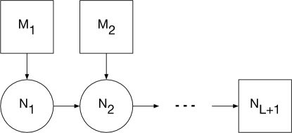
Figure 24: More flavor nodes are attached to the quiver diagram in figure 10.

The 1-loop determinants of the new bi-fundamental chiral multiplets are as follows:

$$\left(\prod_{l=1}^{L}\prod_{i=1}^{M_{l}}\prod_{j=1}^{N_{l}}\frac{\left(\tilde{y}^{(l)}_{i}{x^{(l)}_{j}}^{-1}\right)^{\frac{1}{2}(-m^{(l)}_{j}+1)}}{\left(\tilde{y}^{(l)}_{i}{x^{(l)}_{j}}^{-1}\zeta^{m^{(l)}_{j}};\zeta^{2}\right)_{-m^{(l)}_{j}+1}}\right).$$ (265)

We have additional global symmetries $\prod_{l=1}^{L}U(M_{l})$, whose fugacities are denoted by $\tilde{y}^{(l)}_{i}$. Because the new bi-fundamentals are heading downward, their 1-loop determinants do not develop new contributing poles. Thus, we only need to evaluate the contribution of (265) at the pole (235). The resulting perturbative part and vortex part are as follows:

$$Z^{\text{pert}} =\left(\prod_{l=1}^{L}\prod_{i\neq j}^{N_{l}}\left[y_{\sigma(i)}y_{\sigma(j)}^{-1}\right]\right)\left(\prod_{l=1}^{L}\prod_{i=1}^{N_{l}}\prod_{j=1(\neq i)}^{N_{l+1}}\left[y_{\sigma(i)}y_{\sigma(j)}^{-1}\right]\right)^{-1}\left(\prod_{l=1}^{L}\prod_{i=1}^{M_{l}}\prod_{j=1}^{N_{l}}\left[\tilde{y}^{(l)}_{i}y_{\sigma(j)}^{-1}\right]\right)^{-1},$$ (266)

$$Z^{\text{vort}} =\sum_{n^{(l)}_{i}\geq 0}\left(\prod_{l=1}^{L}\tilde{\xi}_{l}^{\sum_{i}\mathsf{n}^{(l)}_{i}}\right)\left(\prod_{l=1}^{L}\prod_{i\neq j}^{N_{l}}\left[y_{\sigma(i)}y_{\sigma(j)}^{-1};\zeta^{2}\right]_{\mathsf{n}^{(l)}_{i}-\mathsf{n}^{(l)}_{j}}\right)^{-1}$$

$$\quad\times\left(\prod_{l=1}^{L}\prod_{i=1}^{N_{l}}\prod_{j=1}^{N_{l+1}}\left[y_{\sigma(i)}y_{\sigma(j)}^{-1}\zeta^{2};\zeta^{2}\right]_{\mathsf{n}^{(l)}_{i}-\mathsf{n}^{(l+1)}_{j}}\right)^{-1}\left(\prod_{l=1}^{L}\prod_{i=1}^{M_{l}}\prod_{j=1}^{N_{l}}\left[\tilde{y}^{(l)}_{i}y_{\sigma(j)}^{-1};\zeta^{-2}\right]_{\mathsf{n}^{(l)}_{j}}\right).$$ (267)

If we are restricted to $L=1$, this model corresponds to SQCD examined in section 4.1. One can see that (267) agrees with the vortex partition function (69) for $L=1$.

Appendix B Aharony duality for supersymmetric partition functions

We have discussed that the vortex partition is a building block of various 3d supersymmetric partition functions. This is explicitly shown in appendix A for the topologically twisted index. In this regard, the vortex partition function identity we have proven in section 4.1 can be a key ingredient to exhibit the Aharony duality in terms of 3d partition functions. In this appendix, we show that indeed many identities of 3d supersymmetric partition functions can be proven using the vortex partition function identity (4.1) in section 4.1.

For simplicity we focus on the original Aharony duality Aharony:1997gp , i.e., $\kappa=N_{f}-N_{a}=0$. The first example is the superconformal index, a supersymmetric partition function on $S^{2}\times S^{1}$ Bhattacharya:2008zy ; Bhattacharya:2008bja . The superconformal index is defined by

$$I=\mathrm{Tr}~{}(-1)^{F}e^{-\beta^{\prime}\{Q,S\}}x^{E+j}\prod_{i}t_{i}^{F_{i}}.$$ (268)

$Q$ is a supercharge of quantum numbers $E=\frac{1}{2}$, $j=-\frac{1}{2}$ and $R=1$ where those quantum numbers are the Cartans of the bosonic subgroup of the 3d $\mathcal{N}=2$ superconformal group, $SO(2,3)\times SO(2)$. $S$ is another supercharge satisfying $S=Q^{\dagger}$. Only the BPS states saturating

$$\{Q,S\}=E-R-j\geq 0$$ (269)

contribute to the superconformal index. $t_{i}$’s are fugacities for global symmetries commuting with $Q$ and $S$.

The superconformal index can be computed exactly using the supersymmetric localization Kim:2009wb ; Imamura:2011su . It is also shown that the superconformal index is factorized into copies of the vortex partition functions as well as the perturbative part Krattenthaler:2011da ; Hwang:2012jh ; Fujitsuka:2013fga ; Benini:2013yva ; Hwang:2015wna . For our interest, the $\mathcal{N}=2$ $U(N_{c})$ gauge theory with $N_{f}$ pairs of fundamental and anti-fundamental chiral multiplets, the factorization of the superconformal index is worked out in Hwang:2012jh . They also examine the Aharony duality for the factorized index. The equality of the perturbative part is explicitly proven while that of the vortex part is numerically tested. Indeed, their conjectural identity for the vortex part is exactly a special case of our equation (4.1), which we explicitly prove using the vortex wall-crossing interpretation of the Aharony duality. Therefore, combined with their result, (4.1) also proves the superconformal index equality for the Aharony duality.

The second example is the topologically twisted index on $S^{2}\times S^{1}$, which is defined by (229). Its factorization is examined in appendix A. For the $\mathcal{N}=2$ $U(N_{c})$ theory with $N_{f}$ flavors, the (angular momentum refined) twisted index is written in the following factorized form:

$$I=\frac{1}{N_{c}!(N_{f}-N_{c})!}\sum_{\sigma}Z^{\text{pert}}Z^{\text{vort}}Z^{\text{antiv}},$$ (270)

$$Z^{\text{pert}} =\left(\tilde{\xi}^{N_{c}r}\right)\left(\prod_{i=1}^{N_{c}}\prod_{j=N_{c}+1}^{N_{f}}\left[y_{\sigma(i)}y_{\sigma(j)}^{-1}\right]\right)^{-1}\left(\prod_{i=1}^{N_{f}}\prod_{j=1}^{N_{c}}\left[\tilde{y}^{(l)}_{i}y_{\sigma(j)}^{-1}\tau^{-2}\zeta^{2r};\zeta^{2}\right]_{-2r+1}\right)^{-1},$$ (271)

$$Z^{\text{vort}} =\sum_{n_{i}\geq 0}\left(\tilde{\xi}^{\sum_{i}\mathsf{n}_{i}}\right)\left(\prod_{i\neq j}^{N_{c}}\left[y_{\sigma(i)}y_{\sigma(j)}^{-1};\zeta^{2}\right]_{\mathsf{n}_{i}-\mathsf{n}_{j}}\right)^{-1}$$

$$\quad\times\left(\prod_{i=1}^{N_{c}}\prod_{j=1}^{N_{f}}\left[y_{\sigma(i)}y_{\sigma(j)}^{-1}\zeta^{2};\zeta^{2}\right]_{\mathsf{n}_{i}}\right)^{-1}\left(\prod_{i=1}^{N_{f}}\prod_{j=1}^{N_{c}}\left[\tilde{y}_{i}y_{\sigma(j)}^{-1}\tau^{-2}\zeta^{-2r};\zeta^{-2}\right]_{\mathsf{n}_{j}}\right),$$ (272)

$$Z^{\text{antiv}} =\left.Z^{\text{vort}}\right|_{\zeta\rightarrow\zeta^{-1}}$$ (273)

where we have kept $r$, the R-charge of the chiral multiplets, unfixed. $r$ should be an integer due to the topological twist. Also recall that we have defined

$$[a;q]_{n}=a^{-\frac{1}{2}n}q^{-\frac{1}{4}n(n-1)}(a;q)_{n}.$$ (274)

Now we show how each component is identified with the counterpart in the dual theory. For the perturbative part, $Z^{\text{pert}}$, we first observe that the last factor in $Z^{\text{pert}}$ can be rewritten, using

$$\left[a;q\right]_{-n}=\left[aq^{-n};q\right]_{n}^{-1},$$ (275)

as follows:

$$\left(\prod_{i=1}^{N_{f}}\prod_{j=1}^{N_{c}}\left[\tilde{y}^{(l)}_{i}y_{\sigma(j)}^{-1}\tau^{-2}\zeta^{2r};\zeta^{2}\right]_{-2r+1}\right)^{-1}$$

$$=\left(\prod_{i=1}^{N_{f}}\prod_{j=1}^{N_{f}}\left[\tilde{y}^{(l)}_{i}y_{\sigma(j)}^{-1}\tau^{-2}\zeta^{2r};\zeta^{2}\right]_{-2r+1}\right)^{-1}\left(\prod_{i=1}^{N_{f}}\prod_{j=N_{c}+1}^{N_{f}}\left[\tilde{y}^{(l)}_{i}y_{\sigma(j)}^{-1}\tau^{-2}\zeta^{2-2r};\zeta^{2}\right]_{2r-1}\right)^{-1}.$$ (276)

Note that the first factor is exactly the 1-loop determinant of $N_{f}^{2}$ gauge singlet chirals $M_{a}^{\tilde{b}}$ in the dual theory. The second factor corresponds to the contribution of the fundamental chirals in the dual theory. The factor correctly reflects the fact that those fundamental chirals in the dual theory have the R-charge $1-r$. Together with the second factor in $Z^{\text{pert}}$, which can be identified as the contribution of the anti-fundamental chirals in the dual theory, (B) forms the perturbative part of the dual theory up to $\tilde{\xi}$-dependent factors. The $\tilde{\xi}$-dependent factors will be fixed after the vortex parts are taken into account.

Next, let us move on to the vortex parts. Firstly, using

$$[a;q]_{n-m}=\frac{\left[aq^{-m};q\right]_{n}}{\left[aq^{-m};q\right]_{m}},$$ (277)

we rewrite $Z^{\text{vort}}$ in the following form:

$$Z^{\text{vort}} =\sum_{n_{i}\geq 0}\left(\tilde{\xi}^{\sum_{i}\mathsf{n}_{i}}\right)\left(\prod_{i\neq j}^{N_{c}}\left[y_{\sigma(i)}y_{\sigma(j)}^{-1}\zeta^{2\mathsf{n}_{i}};\zeta^{-2}\right]_{\mathsf{n}_{j}}\right)^{-1}$$

$$\quad\times\left(\prod_{i=N_{c}+1}^{N_{f}}\prod_{j=1}^{N_{c}}\left[y_{\sigma(i)}y_{\sigma(j)}^{-1}\zeta^{-2};\zeta^{-2}\right]_{\mathsf{n}_{j}}\right)^{-1}\left(\prod_{i=1}^{N_{f}}\prod_{j=1}^{N_{c}}\left[\tilde{y}_{i}y_{\sigma(j)}^{-1}\tau^{-2}\zeta^{-2r};\zeta^{-2}\right]_{\mathsf{n}_{j}}\right).$$ (278)

Since (B) is nothing but (69), we can use the identity (4.1) with identification $\mathsf{w}=-\tilde{\xi}$. From (4.1), $Z^{\text{vort}}$ and $Z^{\text{antiv}}$ have the following relations with the dual vortex parts, $\bar{Z}^{\text{vort}}$ and $\bar{Z}^{\text{antiv}}$:

$$Z^{\text{vort}} =\bar{Z}^{\text{vort}}\times\mathrm{PE}\left[\frac{\tau^{-N_{f}}\zeta^{-N_{c}+N_{f}(1-r)+1}-\tau^{N_{f}}\zeta^{N_{c}-N_{f}(1-r)+1}}{1-\zeta^{2}}\mathsf{w}\right],$$ (279)

$$Z^{\text{antiv}} =\bar{Z}^{\text{antiv}}\times\mathrm{PE}\left[\frac{\tau^{-N_{f}}\zeta^{N_{c}-N_{f}(1-r)-1}-\tau^{N_{f}}\zeta^{-N_{c}+N_{f}(1-r)-1}}{1-\zeta^{-2}}\mathsf{w}\right].$$ (280)

The product of $Z^{\text{vort}}$ and $Z^{\text{antiv}}$ is then written as

$$Z^{\text{vort}}Z^{\text{antiv}}=\bar{Z}^{\text{vort}}\bar{Z}^{\text{antiv}}\times\mathrm{PE}\left[\left(\mathsf{w}\tau^{-N_{f}}\zeta^{\Delta_{V}}+\mathsf{w}\tau^{N_{f}}\zeta^{\Delta_{V}}\right)\frac{1-\zeta^{-2\Delta_{V}+2}}{1-\zeta^{2}}\right]$$ (281)

where $\Delta_{V}\equiv N_{f}(1-r)-N_{c}+1$ is the R-charge of gauge singlet chirals $V_{\pm}$ in the dual theory. Again $\Delta_{V}$ should be an integer due to the topological twist. One can rewrite the last Plethystic exponential factor as follows:

$$\mathrm{PE}\left[\left(\mathsf{w}\tau^{-N_{f}}\zeta^{\Delta_{V}}+\mathsf{w}\tau^{N_{f}}\zeta^{\Delta_{V}}\right)\frac{1-\zeta^{-2\Delta_{V}+2}}{1-\zeta^{2}}\right]$$

$$=\left(-\mathsf{w}\right)^{\Delta_{V}-1}\left[\mathsf{w}\tau^{-N_{f}}\zeta^{\Delta_{V}};\zeta^{2}\right]_{-\Delta_{V}+1}^{-1}\left[\mathsf{w}^{-1}\tau^{-N_{f}}\zeta^{\Delta_{V}};\zeta^{2}\right]_{-\Delta_{V}+1}^{-1}.$$ (282)

The last two factors are exactly the 1-loop determinants of $V_{\pm}$ in the dual theory. Moreover, the first monomial factor $(-\mathsf{w})^{\Delta_{V}-1}=\tilde{\xi}^{\Delta_{V}-1}$ is combined with the first factor in $Z^{\text{pert}}$ such that we have

$$\tilde{\xi}^{N_{c}r+\Delta_{V}-1}=\tilde{\xi}^{(N_{f}-N_{c})(1-r)},$$ (283)

which is the correct monomial factor that should be included in the dual perturbative part $\bar{Z}^{\text{pert}}$. Thus, (B) and (283) correctly reproduce the $\tilde{\xi}$-dependent factors in $\bar{Z}^{\text{pert}}$, which implies $Z^{\text{pert}}Z^{\text{vort}}Z^{\text{antiv}}=\bar{Z}^{\text{pert}}\bar{Z}^{\text{vort}}\bar{Z}^{\text{antiv}}$. Therefore, the twisted index equality for the Aharony duality is proven using the vortex partition function identity, (4.1).

Our last example is the supersymmetric partition function on the squashed 3-sphere, $S^{3}_{b}$. Using the supersymmetric localization, especially the Higgs branch localization, the partition function is given by the following factorized form Pasquetti:2011fj ; Taki:2013opa ; Fujitsuka:2013fga ; Benini:2013yva :

$$Z=\frac{1}{N_{c}!(N_{f}-N_{c})!}\sum_{\sigma\in S_{N_{c}}}Z^{\text{pert}}Z^{\text{vort}}Z^{\text{antiv}},$$ (284)

$$Z^{\text{pert}}=e^{2\pi i\xi\sum_{i=1}^{N_{c}}(m_{i}+\mu)}$$

$$\times\left(\prod_{i<j}^{N_{c}}4\sinh[\pi b(m_{i}-m_{j})]\sinh[\pi b^{-1}(m_{i}-m_{j})]\right)\frac{\prod_{i=1}^{N_{c}}\prod_{j=1(\neq i)}^{N_{f}}s_{b}(\frac{iQ}{2}+m_{j}-m_{i})}{\prod_{i=1}^{N_{c}}\prod_{j=1}^{N_{f}}s_{b}(-\frac{iQ}{2}+\tilde{m}_{j}-m_{i}-2\mu)},$$ (285)

$$Z^{\text{vort}}=\left.Z^{\text{antiv}}\right|_{b\rightarrow b^{-1}},$$ (286)

$$Z^{\text{antiv}}=\sum_{n_{i}\geq 0}\left((-1)^{N_{f}-N_{c}}e^{2\pi b\xi}\right)^{\sum_{i=1}^{N_{c}}n_{i}}$$

$$\times\prod_{i=1}^{N_{c}}\prod_{l=1}^{n_{i}}\frac{\prod_{j=1}^{N_{f}}2\sinh\pi b(\tilde{m}_{j}-m_{i}-2\mu+(l-1)ib)}{\left(\prod_{j=1}^{N_{c}}2\sinh\pi b(m_{j}-m_{i}+(l-1-n_{j})ib)\right)\left(\prod_{j=N_{c}+1}^{N_{f}}2\sinh\pi b(m_{j}-m_{i}+lib)\right)}$$ (287)

where $s_{b}(z)$ is the double sine function, whose definition can be found in, e.g., Hama:2011ea . $\xi$ is the FI parameter and $m_{j}+\mu$, $\tilde{m}_{j}-\mu$ are mass parameters. $b$ is the squashing parameter of $S^{3}_{b}$ and $Q=b+b^{-1}$. $\sigma$ is a permutation acting on mass parameters $m_{j}$’s.

One should note that the $S^{3}_{b}$ partition function also allows a matrix integral form Hama:2011ea , which is obtained by the Coulomb branch localization. In that case, the Aharony duality is realized as an integral identity of double sine functions Willett:2011gp , which is proven in Bult:2007 . Here we recast the proof of the identity using the vortex partition function.

Firstly we examine the perturbative part. Using double-sine function identities

$$s_{b}(z)s_{b}(-z)=1,$$ (288)

$$s_{b}\left(\frac{iQ}{2}+z\right)=\frac{s_{b}\left(\frac{iQ}{2}+z-ib\right)}{2i\sinh\pi bz},$$ (289)

one can rewrite $Z^{\text{pert}}$ as follows:

$$Z^{\text{pert}}=e^{2\pi i\xi\sum_{i=1}^{N_{c}}(m_{i}+\mu)}\times\frac{\prod_{i=1}^{N_{c}}\prod_{j=N_{c}+1}^{N_{f}}s_{b}(\frac{iQ}{2}+m_{j}-m_{i})}{\prod_{i=1}^{N_{c}}\prod_{j=1}^{N_{f}}s_{b}(-\frac{iQ}{2}+\tilde{m}_{j}-m_{i}-2\mu)}.$$ (290)

The numerator of the second factor appears in the dual perturbative part as it is while the denominator requires a little massage:

$$\prod_{i=1}^{N_{c}}\prod_{j=1}^{N_{f}}s_{b}\left(-\frac{iQ}{2}+\tilde{m}_{j}-m_{i}-2\mu\right)$$

$$=\left(\prod_{i=1}^{N_{f}}\prod_{j=1}^{N_{f}}s_{b}\left(\frac{iQ}{2}-\tilde{m}_{j}+m_{i}+2\mu\right)\right)^{-1}\left(\prod_{i=N_{c}+1}^{N_{f}}\prod_{j=1}^{N_{f}}s_{b}\left(\frac{iQ}{2}-\tilde{m}_{j}+m_{i}+2\mu\right)\right).$$ (291)

(290) combined with (B) produces the perturbative part of the dual theory up to $\xi$-dependent factors, which will be fixed later. Note that the first factor on the right hand side of (B) is the 1-loop determinant of $M_{a}^{\tilde{b}}$ in the dual theory.

Next, we examine the vortex parts. Again, from (4.1), we have the following relations:

$$\begin{aligned} Z^{\text{vort}}&=\bar{Z}^{\text{vort}}\times\mathrm{PE}\left[\frac{\tau^{-N_{f}}\zeta^{-N_{c}+N_{f}+1}-\tau^{N_{f}}\zeta^{N_{c}-N_{f}+1}}{1-\zeta^{2}}\mathsf{w}\right],\\ Z^{\text{antiv}}&=\bar{Z}^{\text{antiv}}\times\left.\mathrm{PE}\left[\frac{\tau^{-N_{f}}\zeta^{-N_{c}+N_{f}+1}-\tau^{N_{f}}\zeta^{N_{c}-N_{f}+1}}{1-\zeta^{2}}\mathsf{w}\right]\right|_{b\rightarrow b^{-1}}\end{aligned}$$ (292)

where $\tau=e^{2\pi b^{-1}\mu}$, $\zeta=e^{-\pi ib^{-2}}$ and $\mathsf{w}=(-1)^{N_{f}-N_{c}+1}e^{2\pi b^{-1}\xi}$. Since the double sine function is written in terms of the Plethystic exponential as follows:

$$s_{b}\left(z+\frac{iQ}{2}\right)=e^{-\frac{i\pi}{2}(z+\frac{iQ}{2})^{2}}\times\mathrm{PE}\left[\frac{e^{2\pi bz}}{1-e^{-2i\pi b^{2}}}+\frac{e^{2\pi b^{-1}z}}{1-e^{-2i\pi b^{-2}}}\right],$$ (293)

the two Plethystic exponentials in (292) together form the following double sine function expression:

$$e^{-2\pi i\xi(N_{f}\mu+\frac{iQ}{2}(N_{f}-N_{c}))}\frac{s_{b}(\xi-N_{f}\mu-\frac{iQ}{2}(N_{f}-N_{c}))}{s_{b}(\xi+N_{f}\mu+\frac{iQ}{2}(N_{f}-N_{c}))}.$$ (294)

Note that the second factor is exactly the 1-loop determinant of $V_{\pm}$ in the dual theory. Combining the monomial factors in (B) and in (294), we have

$$e^{-2\pi i\xi\sum_{i=N_{c}+1}^{N_{f}}(m_{i}+\mu+\frac{iQ}{2})}.$$ (295)

Taking this monomial factor into account, (294) correctly reproduces the $\xi$-dependent factors in the dual perturbative part. Thus, we have proven the identity of the partition functions on $S^{3}_{b}$ for the Aharony duality.

We have shown that three kinds of partition function identities for the Aharony duality can be proven using the identity (4.1) of the vortex partition function. Except the $S^{3}_{b}$ partition function, for which the Aharony duality is proven using an integral identity of the hyperbolic gamma function Bult:2007 ; Willett:2011gp ; Benini:2011mf ; Amariti:2014lla , analytic proofs of the other partition function identities were only available for specific examples with the fixed gauge rank and the fixed number of flavors Krattenthaler:2011da ; Hwang:2012jh or for specific fugacities Closset:2016arn . Our proof, on the other hand, is for the arbitrary gauge rank and the arbitrary number of flavors with full generality of fugacities. The key of our proof is the vortex partition function identity, which is a building block of various 3d partition functions. Thus, our method is not sensitive to the type of a partition function. Furthermore, since those partition functions allow integral expressions, our results can be regarded as proofs of integral identities of special functions.

Our approach is based on the observation of the physical phenomenon, the wall-crossing of vortex quantum mechanics. This shows that a understanding of a physical phenomenon even suggests a new way to prove a nontrivial mathematical identity. Indeed, from various Seiberg-like dualities, there are many conjectural identities beyond what we have proven in this appendix, e.g., Bashkirov:2011vy ; Hwang:2011qt ; Hwang:2011ht ; Kapustin:2011vz ; Cheon:2012be ; Kim:2013cma ; Aharony:2013dha ; Park:2013wta ; Aharony:2013kma ; Gahramanov:gka ; Amariti:2014iza ; Gahramanov:2014ona ; Amariti:2015vwa . A better understanding of physics behind those dualities may give new understandings of various integral identities of special functions. More related discussions are also found in Gahramanov:2013rda ; Gahramanov:2016wxi .

References

- (1) H. Jockers, V. Kumar, J. M. Lapan, D. R. Morrison and M. Romo, Two-Sphere Partition Functions and Gromov-Witten Invariants, Commun. Math. Phys. 325 (2014) 1139–1170, [1208.6244].
- (2) J. Gomis and S. Lee, Exact Kahler Potential from Gauge Theory and Mirror Symmetry, JHEP 04 (2013) 019, [1210.6022].
- (3) F. Benini and S. Cremonesi, Partition Functions of Gauge Theories on S2 and Vortices, Commun. Math. Phys. 334 (2015) 1483–1527, [1206.2356].
- (4) N. Doroud, J. Gomis, B. Le Floch and S. Lee, Exact Results in D=2 Supersymmetric Gauge Theories, JHEP 05 (2013) 093, [1206.2606].
- (5) F. Benini, R. Eager, K. Hori and Y. Tachikawa, Elliptic Genera of 2d = 2 Gauge Theories, Commun. Math. Phys. 333 (2015) 1241–1286, [1308.4896].
- (6) K. Hori, H. Kim and P. Yi, Witten Index and Wall Crossing, JHEP 01 (2015) 124, [1407.2567].
- (7) K. Intriligator and N. Seiberg, Aspects of 3d N=2 Chern-Simons-Matter Theories, JHEP 07 (2013) 079, [1305.1633].
- (8) C. Krattenthaler, V. P. Spiridonov and G. S. Vartanov, Superconformal indices of three-dimensional theories related by mirror symmetry, JHEP 06 (2011) 008, [1103.4075].
- (9) T. Dimofte, D. Gaiotto and S. Gukov, Gauge Theories Labelled by Three-Manifolds, Commun. Math. Phys. 325 (2014) 367–419, [1108.4389].
- (10) S. Pasquetti, Factorisation of N = 2 Theories on the Squashed 3-Sphere, JHEP 04 (2012) 120, [1111.6905].
- (11) C. Beem, T. Dimofte and S. Pasquetti, Holomorphic Blocks in Three Dimensions, JHEP 12 (2014) 177, [1211.1986].
- (12) C. Hwang, H.-C. Kim and J. Park, Factorization of the 3d superconformal index, JHEP 08 (2014) 018, [1211.6023].
- (13) M. Taki, Holomorphic Blocks for 3d Non-abelian Partition Functions, 1303.5915.
- (14) S. Cecotti, D. Gaiotto and C. Vafa, geometry in 3 and 4 dimensions, JHEP 05 (2014) 055, [1312.1008].
- (15) M. Fujitsuka, M. Honda and Y. Yoshida, Higgs branch localization of 3d ?? = 2 theories, PTEP 2014 (2014) 123B02, [1312.3627].
- (16) F. Benini and W. Peelaers, Higgs branch localization in three dimensions, JHEP 05 (2014) 030, [1312.6078].
- (17) F. Benini and A. Zaffaroni, A topologically twisted index for three-dimensional supersymmetric theories, JHEP 07 (2015) 127, [1504.03698].
- (18) N. A. Nekrasov, Seiberg-Witten prepotential from instanton counting, Adv. Theor. Math. Phys. 7 (2003) 831–864, [hep-th/0206161].
- (19) A. Hanany and D. Tong, Vortices, instantons and branes, JHEP 07 (2003) 037, [hep-th/0306150].
- (20) E. J. Weinberg, Fundamental Monopoles in Theories With Arbitrary Symmetry Breaking, Nucl. Phys. B203 (1982) 445–471.
- (21) E. J. Weinberg and P. Yi, Magnetic Monopole Dynamics, Supersymmetry, and Duality, Phys. Rept. 438 (2007) 65–236, [hep-th/0609055].
- (22) F. Denef, Quantum quivers and Hall / hole halos, JHEP 10 (2002) 023, [hep-th/0206072].
- (23) O. Aharony, IR duality in d = 3 N=2 supersymmetric USp(2N(c)) and U(N(c)) gauge theories, Phys. Lett. B404 (1997) 71–76, [hep-th/9703215].
- (24) D. L. Jafferis, The Exact Superconformal R-Symmetry Extremizes Z, JHEP 05 (2012) 159, [1012.3210].
- (25) O. Aharony, A. Hanany, K. A. Intriligator, N. Seiberg and M. J. Strassler, Aspects of N=2 supersymmetric gauge theories in three-dimensions, Nucl. Phys. B499 (1997) 67–99, [hep-th/9703110].
- (26) A. Giveon and D. Kutasov, Seiberg Duality in Chern-Simons Theory, Nucl. Phys. B812 (2009) 1–11, [0808.0360].
- (27) A. Hanany, C. Hwang, H. Kim, J. Park and R.-K. Seong, Hilbert Series for Theories with Aharony Duals, JHEP 11 (2015) 132, [1505.02160].
- (28) S. Cremonesi, The Hilbert series of 3d Yang?Mills theories with vectorlike matter, J. Phys. A48 (2015) 455401, [1505.02409].
- (29) S. Cremonesi, N. Mekareeya and A. Zaffaroni, The moduli spaces of 3d Chern-Simons gauge theories and their Hilbert series, JHEP 10 (2016) 046, [1607.05728].
- (30) E. Witten, Supersymmetric index of three-dimensional gauge theory, hep-th/9903005.
- (31) F. Benini, C. Closset and S. Cremonesi, Comments on 3d Seiberg-like dualities, JHEP 10 (2011) 075, [1108.5373].
- (32) A. Hanany and E. Witten, Type IIB superstrings, BPS monopoles, and three-dimensional gauge dynamics, Nucl. Phys. B492 (1997) 152–190, [hep-th/9611230].
- (33) M. E. Peskin, Mandelstam-’t hooft duality in abelian lattice models, Annals of Physics 113 (1978) 122 – 152.
- (34) C. Dasgupta and B. I. Halperin, Phase transition in a lattice model of superconductivity, Phys. Rev. Lett. 47 (Nov, 1981) 1556–1560.
- (35) D. T. Son, Is the Composite Fermion a Dirac Particle?, Phys. Rev. X5 (2015) 031027, [1502.03446].
- (36) C. Wang and T. Senthil, Dual Dirac Liquid on the Surface of the Electron Topological Insulator, Physical Review X 5 (Oct., 2015) 041031, [1505.05141].
- (37) M. A. Metlitski and A. Vishwanath, Particle-vortex duality of two-dimensional Dirac fermion from electric-magnetic duality of three-dimensional topological insulators, Phys. Rev. B93 (2016) 245151, [1505.05142].
- (38) K. A. Intriligator and N. Seiberg, Mirror symmetry in three-dimensional gauge theories, Phys. Lett. B387 (1996) 513–519, [hep-th/9607207].
- (39) A. Kapustin and M. J. Strassler, On mirror symmetry in three-dimensional Abelian gauge theories, JHEP 04 (1999) 021, [hep-th/9902033].
- (40) A. Karch and D. Tong, Particle-Vortex Duality from 3d Bosonization, Phys. Rev. X6 (2016) 031043, [1606.01893].
- (41) J. Murugan and H. Nastase, Particle-vortex duality in topological insulators and superconductors, 1606.01912.
- (42) N. Seiberg, T. Senthil, C. Wang and E. Witten, A Duality Web in 2+1 Dimensions and Condensed Matter Physics, Annals Phys. 374 (2016) 395–433, [1606.01989].
- (43) S. Kachru, M. Mulligan, G. Torroba and H. Wang, Bosonization and Mirror Symmetry, Phys. Rev. D94 (2016) 085009, [1608.05077].
- (44) S. Kachru, M. Mulligan, G. Torroba and H. Wang, The many faces of mirror symmetry, Phys. Rev. Lett. 118 (2017) 011602, [1609.02149].
- (45) D. Gaiotto and E. Witten, S-Duality of Boundary Conditions In N=4 Super Yang-Mills Theory, Adv. Theor. Math. Phys. 13 (2009) 721–896, [0807.3720].
- (46) A. Kapustin, B. Willett and I. Yaakov, Tests of Seiberg-like Duality in Three Dimensions, 1012.4021.
- (47) H.-C. Kim, J. Kim, S. Kim and K. Lee, Vortices and 3 dimensional dualities, 1204.3895.
- (48) I. Yaakov, Redeeming Bad Theories, JHEP 11 (2013) 189, [1303.2769].
- (49) D. Gaiotto and P. Koroteev, On Three Dimensional Quiver Gauge Theories and Integrability, JHEP 05 (2013) 126, [1304.0779].
- (50) E. Witten, Constraints on Supersymmetry Breaking, Nucl. Phys. B202 (1982) 253.
- (51) L. Alvarez-Gaume, SUPERSYMMETRY AND INDEX THEORY, in 1984 NATO ASI on Supersymmetry Bonn, Germany, August 20-31, 1984, pp. 1–44, 1986.
- (52) S.-J. Lee and P. Yi, Witten Index for Noncompact Dynamics, JHEP 06 (2016) 089, [1602.03530].
- (53) C. Hwang, J. Kim, S. Kim and J. Park, General instanton counting and 5d SCFT, JHEP 07 (2015) 063, [1406.6793].
- (54) C. Cordova and S.-H. Shao, An Index Formula for Supersymmetric Quantum Mechanics, 1406.7853.
- (55) L. C. Jeffrey and F. C. Kirwan, Localization for nonabelian group actions, in eprint arXiv:alg-geom/9307001, July, 1993.
- (56) M. Brion and M. Vergne, Arrangements of hyperplanes I: Rational functions and Jeffrey-Kirwan residue, ArXiv Mathematics e-prints (Mar., 1999) , [math/9903178].
- (57) A. Szenes and M. Vergne, Toric reduction and a conjecture of Batyrev and Materov, Inventiones Mathematicae 158 (June, 2004) 453–495, [math/0306311].
- (58) M. Aganagic, N. Haouzi and S. Shakirov, -Triality, 1403.3657.
- (59) M. Bullimore, T. Dimofte, D. Gaiotto, J. Hilburn and H.-C. Kim, Vortices and Vermas, 1609.04406.
- (60) M. Bullimore, H.-C. Kim and P. Koroteev, Defects and Quantum Seiberg-Witten Geometry, JHEP 05 (2015) 095, [1412.6081].
- (61) S. Nawata, Givental J-functions, Quantum integrable systems, AGT relation with surface operator, Adv. Theor. Math. Phys. 19 (2015) 1277–1338, [1408.4132].
- (62) M. Finkelberg and L. Rybnikov, Quantization of Drinfeld Zastava in type A, J. Eur. Math. Soc. (JEMS) 16 (2014) 235–271, [1009.0676].
- (63) S. Venugopalan and C. T. Woodward, Classification of affine vortices, Duke. Math. J 165 (2016) 1695–1751, [1301.7052].
- (64) A. Givental and Y.-P. Lee, Quantum K-theory on flag manifolds, finite-difference Toda lattices and quantum groups, Inventiones Mathematicae. 151 (2003) 193?219, [math/0108105].
- (65) T. Dimofte, S. Gukov and L. Hollands, Vortex Counting and Lagrangian 3-manifolds, Lett. Math. Phys. 98 (2011) 225–287, [1006.0977].
- (66) C. Hwang and J. Park, Factorization of the 3d superconformal index with an adjoint matter, JHEP 11 (2015) 028, [1506.03951].
- (67) B. Willett and I. Yaakov, N=2 Dualities and Z Extremization in Three Dimensions, 1104.0487.
- (68) A. Amariti and C. Klare, Chern-Simons and RG Flows: Contact with Dualities, JHEP 08 (2014) 144, [1405.2312].
- (69) F. van de Bult, Hyperbolic Hypergeometric Functions, Thesis (2007) .
- (70) C. Closset and H. Kim, Comments on twisted indices in 3d supersymmetric gauge theories, JHEP 08 (2016) 059, [1605.06531].
- (71) S. Kim, The Complete superconformal index for N=6 Chern-Simons theory, Nucl. Phys. B821 (2009) 241–284, [0903.4172].
- (72) A. Kapustin, B. Willett and I. Yaakov, Exact Results for Wilson Loops in Superconformal Chern-Simons Theories with Matter, JHEP 03 (2010) 089, [0909.4559].
- (73) N. Hama, K. Hosomichi and S. Lee, Notes on SUSY Gauge Theories on Three-Sphere, JHEP 03 (2011) 127, [1012.3512].
- (74) Y. Imamura and S. Yokoyama, Index for three dimensional superconformal field theories with general R-charge assignments, JHEP 04 (2011) 007, [1101.0557].
- (75) N. Hama, K. Hosomichi and S. Lee, SUSY Gauge Theories on Squashed Three-Spheres, JHEP 05 (2011) 014, [1102.4716].
- (76) A. Kapustin and B. Willett, Generalized Superconformal Index for Three Dimensional Field Theories, 1106.2484.
- (77) F. Benini, T. Nishioka and M. Yamazaki, 4d Index to 3d Index and 2d TQFT, Phys. Rev. D86 (2012) 065015, [1109.0283].
- (78) Y. Imamura and D. Yokoyama, N=2 supersymmetric theories on squashed three-sphere, Phys. Rev. D85 (2012) 025015, [1109.4734].
- (79) L. F. Alday, M. Fluder and J. Sparks, The Large N limit of M2-branes on Lens spaces, JHEP 10 (2012) 057, [1204.1280].
- (80) F. Benini and A. Zaffaroni, Supersymmetric partition functions on Riemann surfaces, 1605.06120.
- (81) J. Bhattacharya, S. Bhattacharyya, S. Minwalla and S. Raju, Indices for Superconformal Field Theories in 3,5 and 6 Dimensions, JHEP 02 (2008) 064, [0801.1435].
- (82) J. Bhattacharya and S. Minwalla, Superconformal Indices for N = 6 Chern Simons Theories, JHEP 01 (2009) 014, [0806.3251].
- (83) D. Bashkirov, Aharony duality and monopole operators in three dimensions, 1106.4110.
- (84) C. Hwang, H. Kim, K.-J. Park and J. Park, Index computation for 3d Chern-Simons matter theory: test of Seiberg-like duality, JHEP 09 (2011) 037, [1107.4942].
- (85) C. Hwang, K.-J. Park and J. Park, Evidence for Aharony duality for orthogonal gauge groups, JHEP 11 (2011) 011, [1109.2828].
- (86) A. Kapustin, H. Kim and J. Park, Dualities for 3d Theories with Tensor Matter, JHEP 12 (2011) 087, [1110.2547].
- (87) S. Cheon, D. Gang, C. Hwang, S. Nagaoka and J. Park, Duality between N=5 and N=6 Chern-Simons matter theory, JHEP 11 (2012) 009, [1208.6085].
- (88) H. Kim and J. Park, Aharony Dualities for 3d Theories with Adjoint Matter, JHEP 06 (2013) 106, [1302.3645].
- (89) O. Aharony, S. S. Razamat, N. Seiberg and B. Willett, 3d dualities from 4d dualities, JHEP 07 (2013) 149, [1305.3924].
- (90) J. Park and K.-J. Park, Seiberg-like Dualities for 3d N=2 Theories with SU(N) gauge group, JHEP 10 (2013) 198, [1305.6280].
- (91) O. Aharony, S. S. Razamat, N. Seiberg and B. Willett, 3 dualities from 4 dualities for orthogonal groups, JHEP 08 (2013) 099, [1307.0511].
- (92) I. B. Gahramanov and G. S. Vartanov, Superconformal indices and partition functions for supersymmetric field theories, in XVIIth Intern. Cong. Math. Phys. 695-703 (2013), 2013. 1310.8507. DOI.
- (93) A. Amariti and C. Klare, A journey to 3d: exact relations for adjoint SQCD from dimensional reduction, JHEP 05 (2015) 148, [1409.8623].
- (94) I. Gahramanov and H. Rosengren, Integral pentagon relations for 3d superconformal indices, 1412.2926.
- (95) A. Amariti, Integral identities for 3d dualities with SP(2N) gauge groups, 1509.02199.
- (96) I. Gahramanov and H. Rosengren, A new pentagon identity for the tetrahedron index, JHEP 11 (2013) 128, [1309.2195].
- (97) I. Gahramanov and H. Rosengren, Basic hypergeometry of supersymmetric dualities, Nucl. Phys. B913 (2016) 747–768, [1606.08185].