Two New Contributions to the Visualization of AMR Grids:
I. Interactive Rendering of Extreme-Scale $2$-Dimensional Grids
II. Novel Selection Filters in Arbitrary Dimension

Abstract

We present here the result of continuation work, performed to further fulfill the vision we outlined in harel:17 for the visualization and analysis of tree-based adaptive mesh refinement (AMR) simulations, using the hypertree grid paradigm which we proposed.

The first filter presented hereafter implements an adaptive approach in order to accelerate the rendering of $2$-dimensional AMR grids, hereby solving the problem posed by the loss of interactivity that occurs when dealing with large and/or deeply refined meshes. Specifically, view parameters are taken into account, in order to: on one hand, avoid creating surface elements that are outside of the view area; on the other hand, utilize level-of-detail properties to cull those cells that are deemed too small to be visible with respect to the given view parameters. This adaptive approach often results in a massive increase in rendering performance.

In addition, two new selection filters provide data analysis capabilities, by means of allowing for the extraction of those cells within a hypertree grid that are deemed relevant in some sense, either geometrically or topologically. After a description of these new algorithms, we illustrate their use within the Visualization Toolkit (VTK) in which we implemented them. This note ends with some suggestions for subsequent work.

1 Introduction

This short article is a sequel to harel:17 , where we presented the first systematic treatment of the problems posed by the visualization and analysis of large-scale, parallel, tree-based adaptive mesh refinement (AMR) simulations on an Eulerian grid. In that previous article, we proposed a novel data object for the Visualization Toolkit (VTK) avila:10 , able to support all conceivable types of rectilinear, tree-based AMR data sets not only produced by today’s simulation software, but also by what is foreseeable of tomorrow’s extreme-scale simulations.

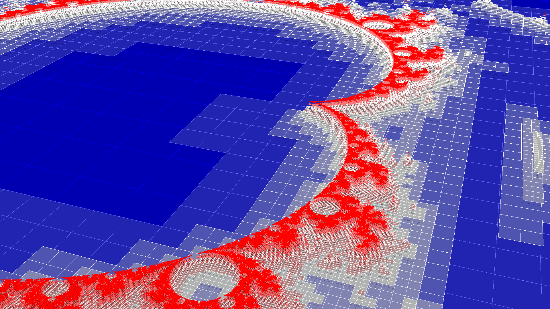
Figure 1: Visualization of the different levels of a $2$-dimensional AMR grid, whose depth levels are raised by increasing elevations in order to highlight the hierarchic nature of the object.

The concrete result of this earlier work is a novel version of the vtkHyperTreeGrid data object, differing in many key aspects from the initial incarnation which we proposed in carrard:imr21 . The novel version also includes a dozen of visualizations algorithms (filters) operating natively upon the new data object. An example visualization obtained with this new object is shown in Figure 1. Note that this set of filters includes, in particular, a conversion algorithm to transform a tree-based AMR grid into a fully explicit, unstructured mesh that can, albeit extremely inefficiently, be processed by other visualization techniques not currently included in the native, hypertree grid filter. One key aspect of this improved object is that it relies on a hierarchy of templated traversal objects, called cursors and supercursors, allowing for the easy creation of new filters while retaining the intrinsic performance of our method, in terms of both execution speed and memory footprint.

Meanwhile, we acknowledged that $2$-dimensional AMR visualization could be especially challenging, as a result of its requirement that all leaf cells be rendered. This constraint makes the interactivity of the visualization process decrease as input data object size increases. It is important to note that this problem is further compounded by the enhanced efficiency, in terms of memory footprint, of our hypertree grid model. This elicits a new situation where rendering has become the bottleneck for the target platforms.

As a result, our next stated goal was to optimize rendering speed, in order to maintain interactivity when visualizing the largest possible tree grids that can be contained in memory. We thus set out to address this urgent need, for which the lack of existing solution was hindering the AMR visualization and analysis workflow. The results of this work are thus presented hereafter.

In addition, we also explain here how we expanded the set of hypertree grid filters with two novel data selection and extraction filters: one based on location (i.e., a geometric property), the other on element Id (i.e., a topological property). This further supports, in particular, our claim that the new hypertree grid framework offers enough flexibility and convenience that algorithms not initially envisioned can be readily added and deployed.

2 Method

2.1 Adaptive Dataset Surface Filter

The purpose of this filter is to extract the outer surface of an hyper tree grid. It is worth noting that the Geometry filter already provides this capability, cf.harel:17 . However, an additional constraint is added, namely an emphasis on rendering speed in dimension $2$. Our method to address this need is to exploit level-of-detail properties, culling those parts of the data set that are not visible, i.e., not contained in the visualization frustum formed by the camera and object positions. The algorithm explores each tree in the grid, searching for those faces of the different leaf cells that belong to the surface. At the end of the computation, the result is a polygonal mesh (concretely, a vtkPolyData instance) containing an array of rectangular cells, that can be used to render the surface of the hyper tree.

The main difference between this adaptive geometry filter and the non-adaptive one is that it allows for the use of the renderer parameters to reduce the computational work. Note that currently, this feature is only available when working with a $2$-dimensional mesh and a parallel projection is set. When working under these circumstances, the filter computes only the part of the surface of the grid that is going to be rendered. This also means that whenever any of the parameters of the camera associated to the renderer are modified, the output surface must be subsequently recomputed.

In order to traverse a $2$-dimensional hypertree grid, the algorithm uses a geometric cursor. We briefly recall here that this cursor provides information about the size and the coordinates of the cells of the tree and the number of children, cf.harel:17 for details. The algorithm then recursively processes the entire tree, cell by cell starting from the root level and using a depth-first search (DFS) order. In order to cull those cells that are below a certain size in the rendering window, the DFS traversal is not allowed to descend below the following maximum depth:

$$\delta_{\max}(w,z,s,f)=\frac{\log(wz)-\log{s}}{\log{f}}$$ (1)

where $w$, $z$, $s$ and $f$ respectively denote the size, zoom-in factor, scale of the rendering window, and the branching factor of the hypertree grid.

If the cell to be processed is outside of the rendering area, it is discarded, which results in reducing the amount of computational work to be performed by the algorithm. Non-leaf cells only need to recursively process their children. Leaf cells are processed, unless they are masked, in which case they shall not participate in the output surface. If a cell is not masked, its geometry and topology are computed, and these are added to the list of points and cells defining the polygonal mesh output.

When the input is a $3$-dimensional hyper tree grid we find a different situation, as we only want to generate the outer surface we need to omit internal surfaces: in this case, the same method as that used by the Geometry filter is used.

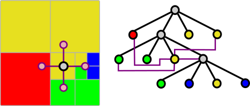
Figure 2: Von Neumann supercursor of a cell that has neighbors with arbitrary depths, in a $3$-deep, $2$-dimensional binary AMR mesh.

This information can be readily retrieved when using a Von Neumann supercursor, as illustrated in Figure 2 (cf. harel:17 for details). Once again, we start processing the tree from the root level. If the cell that we are processing is a non-leaf cell we recursively process its children. Once arrived at a leaf cell, each of its 6 faces (as the cell is then viewed as a rectangular prism) is analyzed: if a face belongs to an unmasked cell and has no neighbor or the neighbor is masked, then that face belongs to the surface to be generated. In this case, its geometry and topology are computed and appended to the list of quadrangles defining the output geometry. Note that the $3$-dimensional case of this filter is identical to that of the Geometry filter which we implemented, as renderer information is taken into account in this case.

2.2 Selection Extraction Filter

In order to extend the set of filters operating on hypertree grids to include data analysis capabilities, we started by extending the selection and extraction methodology of VTK so it can natively operate on hypertree grids. We recall that extraction filters are designed to generate subsets of cells from an input mesh, based on some selection process. In terms of implementation, the object to be processed is sent to the first input port of the filter, whereas the selection, i.e. an instance of a vtkSelection object, is given to a second port. This is a first difference with all hypertree grid filters that we implemented so far, which operate on a single input, and therefore only make use of a single input port. In addition, we wanted to support two different kind of selection modes: by location (i.e., a geometric criterion) and by identifier (i.e., a topological criterion).

When the selection mode is by location, the user must provides a list of coordinates. The algorithm then recursively explores the tree using a geometric cursor until it reaches a leaf cell, again using DFS traversal. In this mode of operation, only non-masked leaf cells can be selected, so all others are ignored. A geometric cursor is also used, so that size and position of selected cells can be easily retrieved. The algorithm then checks whether any of these locations are contained inside each of the traversed cell limits. In this case, the cell is selected, and the filter can return two kinds of outputs: if the PreserveTopology flag is set to true, then the selection process is made by means of a mask array attached to the grid. We recall that such an array associates a value for every cell of the input hyper tree grid, with value of $1$ for selected cells and a value of $0$ for non-selected cells. On the other hand, when the PreserveTopology flag is not set, the output result is an unstructured grid containing all selected cells. In the $2$-dimensional case, this output grid is made of VTK_QUAD elements, whereas in the $3$-dimensional it only contains VTK_HEXAHEDRON cells.

The other mode of operation of the filter is when the vtkSelection is a list of identifiers (Ids). In this case, the algorithm is going to search the tree, looking for these Ids. Starting from the root cells of the hypertree grid, each constituting tree is traversed in DFS order. Given a cell that is not masked by the material mask array, we compare its global Id with the values contained in the list of identifiers. If the cell is in the array, it should be selected, otherwise we keep recursively searching through its children. We use again a geometric cursor because we need to compute the coordinates of the points of the selected cells, as with the other mode of operation. Here also, the output of the filter is an unstructured grid containing VTK_QUAD cells in the $2$-dimensional case, and VTK_HEXAHEDRON cells in the $3$-dimensional case.

3 Results

We now discuss the main results obtained with our implementation in VTK of the previously described new hypertree grid filters.

3.1 Adaptive Surface Filter

We begin with the adaptive geometry extraction filter introduced in §2.1 and implemented in VTK, exploring the $2$ and $3$-dimensional cases as well as the two possible branch factor values.

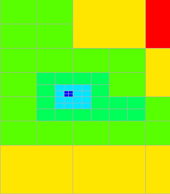
(a)

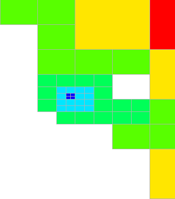
(b)

Figure 3: Visualizations of a part of the data sets produced by the application of the AdaptiveDataSetSurface filter to a $2$-dimensional, binary hypertree grid with 6 root cells, without (a) or with (b) a material mask; only cells that are visible based on camera and object position are generated.

Figure 3 displays renderings obtained by applying the AdaptiveDataSetSurface filter to a 2-dimensional binary hypertree grid, with a $2\times 3$ layout of root cells, to which is attached a single attribute field filled with the cell depths, either without (a) or with (b) a non-empty material mask attached to it. We acknowledge that the adaptive surface filter did indeed compute a reduced number of polygons, with respect to the non-adaptive Geometry filter: specifically, where the entire $2$-dimensional AMR mesh has $75$ leaf cells, the output of AdaptiveDataSetSurface contains only $67$ quadrangles. When a material mask is present, the corresponding numbers are $62$ and $54$, respectively. In the latter case, the gain is inferior to that of the former, as a result of the fact that most culling is due to the masking rather than to the camera position relative to object.

Figure 4: Successive close-up renderings of a $2$-dimensional AMR grid obtained with the AdaptiveDataSetSurface filter.

The elimination of those polygons that are outside the rendering window or, more precisely, their non-creation, is further illustrated in Figure 4 with the example of a $2$-dimensional hypertree grid data set resulting from a computational fluid dynamics simulation.

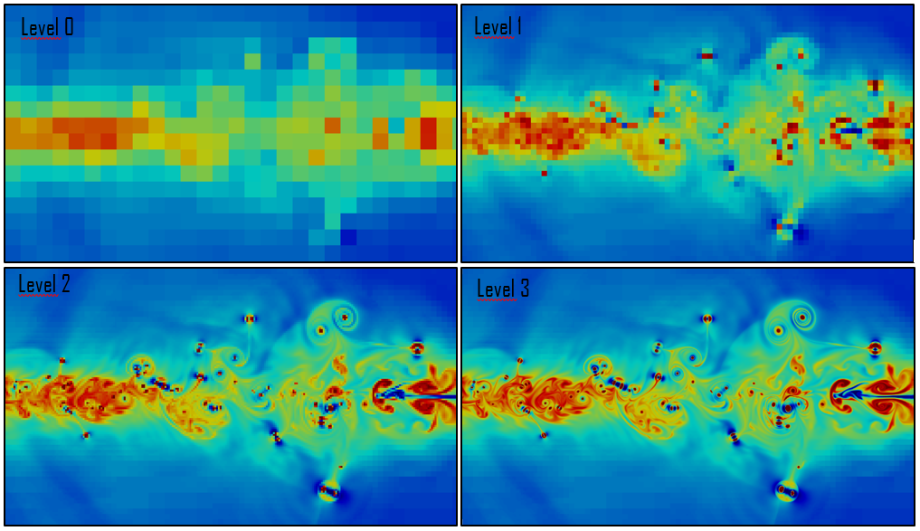
Figure 5: Renderings of a $2$-dimensional AMR grid obtained with the AdaptiveDataSetSurface filter, showing the effect of a decreasing pixelization threshold.

The sub-pixel culling effect of the adaptive surface filter is illustrated in Figure 5, again with a $2$-dimensional hypertree grid, where we can see the effect of adjusting the scale factor $s$ in (1):

$$s_{1}>s_{2} \Leftrightarrow -\log{s_{1}}<-\log{s_{2}}$$

$$\Leftrightarrow \delta_{\max}(w,z,s_{1},f)<\delta_{\max}(w,z,s_{2},f)\ .$$

In other words, increasing the scale factor results in decreasing the maximum allowable depth in the DFS traversals of each of the constituting hypertrees, meaning that more down-sampling will occur. The same effect obviously occurs when instead of increasing $s$, either the window size $w$ is decreased, or the view is zoomed out.

Figure 6: Renderings of the outside surface of $3$-dimensional, ternary hypertree grid with 18 root cells, using the AdaptiveDataSetSurface, without (left) or with (right) a non-empty material mask.

A $3$-dimensional, ternary set of test cases is now used, with a $3\times 3\times 2$ layout of roots to further illustrate our point. We illustrate this in Figure 6, without or with the presence of a non-empty material mask. We note in particular that in this case, the visualizations obtained using the novel AdaptiveDataSetSurface filter are indeed identical to those obtained with the Geometry filter, cf. harel:17 for details; in addition, no culling in the surface geometry occurred as expected.

3.2 Selection Extraction Filters

(a)

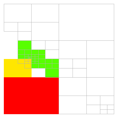
(c)

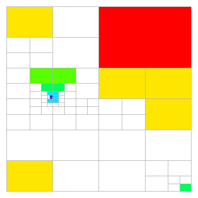
(b)

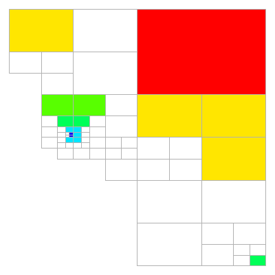
(d)

Figure 7: Visualizations of a part of the unstructured data sets produced by the application of the ExtractSelectedIds (a&c) and ExtractSelectedLocations (b&d) filters to a $2$-dimensional, binary hypertree grid with 6 root cells, without (a&b) or with (c&d) a material mask.

We continue with the selection extraction filter introduced in §2.2 and also implemented in VTK, exploring the $2$ and $3$-dimensional cases as well as the two possible branch factor values. Using the same 2-dimensional binary hypertree grid with a $2\times 3$ layout of root cells, as in §3.1 Figure 7 displays the renderings obtained with the selection extraction filters applied to this hypertree grid, either with or without a non-empty material mask attached to it.

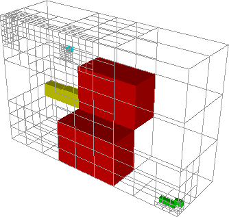
(a)

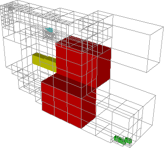
(c)

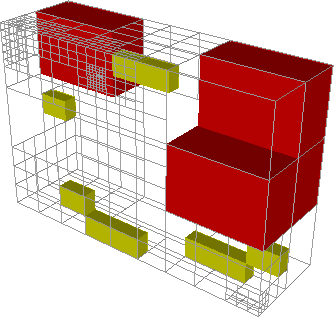
(b)

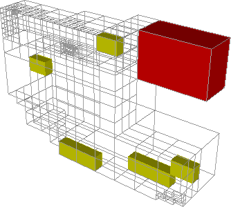
(d)

Figure 8: Visualizations of a part of the unstructured data sets produced by the application of the ExtractSelectedIds (a&c) and ExtractSelectedLocations (b&d) filters to a $3$-dimensional, ternary hypertree grid with 18 root cells, without (a&b) or with (c&d) a material mask.

Finally, the same $3$-dimensional, ternary hypertree grid with a $3\times 3\times 2$ layout of root cells as in §3.1 is used to further illustrate our point in Figure 8. Furthermore, these baseline comparisons are done with the presence of a non-empty material mask, as well as without.

The interested reader is invited to draw parallels between corresponding $2$ and $3$ dimensional sub-figures, and to inspect the contents of the test harness we implemented for all existing hypertree grid filters, across different dimensions and branching factors: 8 new individual tests are available and can be either executed as they are, or modified and experimented with at will. Of particular interest is the behavior of these filters in the presence of a material mask, allowing for the selection of masked out cells. This can be seen in both $2$ and $3$-dimensional cases and is not a bug, but a desired feature.

4 Conclusion

In this article we provided a description of the new native hypertree grid filters which we developed, in order to further advance the vision which we had outlined in harel:17 . One of these two filters implements an efficient version of a commonly used visualization technique, whereas the two other ones already belong to the field of data analysis: indeed, these offer the ability to drill into simulation data sets, and extract from them those parts that are considered relevant either topologically or geometrically. These three new filters have been incorporated into the set of native hypertree grid filters, and we are planning to release them as part of the open-source VTK library.

For future work, we are considering on one hand to extend the AdaptiveDataSetSurface filter to support level-of-detailed rendering for the $3$-dimensional case as well. Note that we first focused on the $2$-dimensional implementation first, because this is the case where performance gains are the highest in relative terms. This is a result of the fact that, by definition, no culling occurs when showing the outside surface of planar data set, whereas in dimension $3$ only boundary cells can produce surface rectangles. On the other hand, another selection extraction filter, using attribute values instead of data set geometry or topology, would be a useful addition the current data analysis capabilities of the tool set.

Acknowledgments

This work was supported by the French Alternative Energies and Atomic Energy Commission (CEA), Directorate of Military Applications (DAM). We thank J.-C. Frament (Positiveyes) for the helpful discussions in the context of this work.

References

- [1] L. Avila, U. Ayachit, S. Barré, J. Baumes, F. Bertel, R. Blue, D. Cole, D. DeMarle, B. Geveci, W. Hoffman, B. King, K. Krishnan, C. Law, K. Martin, W. McLendon, P. Pébaÿ, N. Russell, W. Schroeder, T Shead, J. Shepherd, A. Wilson, and B. Wylie. The VTK User’s Guide. Kitware, Inc., eleventh edition, 2010.
- [2] T. Carrard, C. Law, and P. Pébaÿ. A generic hyper tree grid implementation for AMR mesh manipulation and visualization in VTK. In Proc. 21st International Meshing Roundtable, San Jose, CA, U.S.A., October 2012.
- [3] G. Harel, J.-B. Lekien, and P. P. Pébaÿ. Visualization and analysis of large-scale, tree-based, adaptive mesh refinement simulations with arbitrary rectilinear geometry. arXiv:1702.04852, February 2017.