Signatures of quantum phase transitions from the boundary of the numerical range

Abstract.

The ground state energy of a finite-dimensional one-parameter Hamiltonian and the continuity of a maximum-entropy inference map are discussed in the context of quantum critical phenomena. The domain of the inference map is a convex compact set in the plane, called the numerical range. We study the differential geometry of its boundary in relation to the ground state energy. We prove that discontinuities of the inference map correspond to $C^{1}$-smooth crossings of the ground state energy with a higher energy level. Discontinuities may appear only at $C^{1}$-smooth points of the boundary of the numerical range considered as a manifold. Discontinuities exist at all $C^{2}$-smooth non-analytic boundary points and are essentially stronger than at analytic points or at points which are merely $C^{1}$-smooth (non-exposed points).

Signatures of quantum phase transitions

1. Introduction

Quantum phase transitions are associated with the ground state of an infinite lattice system [61, 48] and are marked by non-analyticity of the ground state energy, energy level crossing with the ground state energy, or long-range correlation in the ground state. Quantum phase transitions have been witnessed in terms of entropy of entanglement [73, 42], which quantifies quantum mechanical correlations.

Signatures of quantum phase transitions were identified already in finite lattices without a thermodynamic limit. They include strong variation [3] and discontinuity [17] of maximum-entropy inference maps, geometry of reduced density matrices [28, 82, 18], or responsiveness of entropic correlation quantities [50]. Our focus are the eigenvalue crossings of a one-parameter Hamiltonian,

$$H(g):=H_{0}+g\cdot H_{1},\qquad g\in\mathbb{R},$$

acting on the Hilbert space $\mathbb{C}^{d}$, $d\in\mathbb{N}$ (independent of a specific lattice model). We think of the energy operators $H_{0},H_{1}\in M_{d}^{\rm h}$ as an unperturbed Hamiltonian $H_{0}$ to which an external field $H_{1}$ is coupled. Here $M_{d}^{\rm h}$ denotes the real space of hermitian matrices of the C*-algebra $M_{d}$ of $d$-by-$d$ matrices.

Let $\mathcal{M}_{d}$ denote the state space [2] of $M_{d}$, which is the set of positive semi-definite matrices of trace one in $M_{d}$, called density matrices. The expected value [8] of $a\in M_{d}^{\rm h}$, interpreted as energy operator, is $\operatorname{tr}(\rho a)$ if the system is in the state $\rho\in\mathcal{M}_{d}$. The set of simultaneous expected values of $H_{0}$ and $H_{1}$,

$$\{(\operatorname{tr}\rho H_{0},\operatorname{tr}\rho H_{1}):\rho\in\mathcal{M}_{d}\},$$

is a projection of $\mathcal{M}_{d}$ to the plane.

It is convenient to use $A=H_{0}+\operatorname{i}H_{1}$ rather than $H(g)$, which is recovered from the real part $H_{0}=\operatorname{Re}A$ and the imaginary part $H_{1}=\operatorname{Im}A$ of $A$, where

$$\operatorname{Re}A=\tfrac{1}{2}(A+A^{*})\qquad\mbox{and}\qquad\operatorname{Im}A=\tfrac{1}{2\operatorname{i}}(A-A^{*}).$$

Using Dirac notation, the numerical range of $A$,

$$W:=W_{A}:=\{\langle x|Ax\rangle:|x\rangle\in\mathbb{C}^{d},\langle x|x\rangle=1\},$$

is a convex subset of $\mathbb{C}$ by a theorem of Toeplitz and Hausdorff [72, 31]. The numerical range is a compact, convex, and non-empty subset of $\mathbb{C}\cong\mathbb{R}^{2}$, a class of sets called convex bodies [63]. The numerical range of $A$ equals the projection [9]

$$W_{A}=\{\operatorname{tr}(\rho A):\rho\in\mathcal{M}_{d}\}$$

of the state space $\mathcal{M}_{d}$, which is the set of expected values of $H_{0}$ and $H_{1}$.

The parameter $h$ of $H(g)$ is shifted to $A$ by introducing an angular coordinate $\theta\in\,]-\tfrac{\pi}{2},\tfrac{\pi}{2}[\,$, for which one finds

(1.1) $$\operatorname{Re}(e^{-\operatorname{i}\theta}A)=H_{0}\cos\theta+H_{1}\sin\theta=H(\tan\theta)\cos\theta.$$

Let $\lambda(\theta)$ denote the smallest eigenvalue of $\operatorname{Re}(e^{-\operatorname{i}\theta}A)$. For unit vectors $|\phi\rangle,|\psi\rangle\in\mathbb{C}^{d}$, such that $|\psi\rangle$ is an eigenvector of $\operatorname{Re}(e^{-\operatorname{i}\theta}A)$ corresponding to $\lambda(\theta)$, we have [72]

(1.2) $$\lambda(\theta)=\langle\psi|\operatorname{Re}(e^{-\operatorname{i}\theta}A)\psi\rangle\leq\langle\phi|\operatorname{Re}(e^{-\operatorname{i}\theta}A)\phi\rangle=\operatorname{Re}\langle e^{\operatorname{i}\theta}|\langle\phi|A\phi\rangle\rangle.$$

Using the Euclidean scalar product $\langle z_{1},z_{2}\rangle=\operatorname{Re}\langle z_{1}|z_{2}\rangle$ of $z_{1},z_{2}\in\mathbb{C}$, equation (1.2) shows that $\lambda(\theta)$ is the support function of $W$ evaluated at $e^{\operatorname{i}\theta}$. This means that $\lambda(\theta)$ is the signed distance $\lambda(\theta)=\min_{z\in W}\langle e^{\operatorname{i}\theta},z\rangle$ of the origin from the supporting line of $W$ with inner normal vector $e^{\operatorname{i}\theta}$.

In physics, the smallest eigenvalue of $H(g)$ is the ground state energy of $H(g)$ and the corresponding eigenspace is the ground space. By virtue of (1.1) the ground state energy at $g\in\mathbb{R}$ is $\sqrt{1+g^{2}}\cdot\lambda(\arctan g)$. Its maximal order of continuous differentiability at $g$ is the same as that of $\lambda$ at $\arctan g$. Therefore is suffices to discus $\lambda$ and and its crossings with the eigenvalues of $\operatorname{Re}(e^{-\operatorname{i}\theta}A)$ which form a set of analytic curves [59].

Although the differential geometry of the boundary $\partial W$ was studied before [29], finite-order differentiability was not addressed. We show that the maximal order of differentiability of the smallest eigenvalue $\lambda$ is even and equal to that of $\partial W$, viewed as a submanifold of $\mathbb{C}$, at corresponding points. Non-analytic points of class $C^{2}$ exist [45, 46] if $d\geq 4$, we return to them later. We use the reverse Gauss map $x_{W}$ to compare maximal orders, thereby viewing $\partial W$ as an envelope of supporting lines and as a manifold. By definition, every unit vector $u\in\mathbb{C}$ which is the inner normal vector of a supporting line of $W$ meeting $W$ at a single point $z$ belongs to the domain of $x_{W}$ and the value is $x_{W}(u):=z$. A point of $W$ is an exposed point if it lies in the image of $x_{W}$. Suitably restricted, the inverse of $x_{W}$ is the Gauss map which sends smooth boundary points to normal vectors. That $\partial W$ is an envelope means that $x_{W}$ is the gradient of the support function of $W$, see [71] or [12]. Hence, that $x_{W}$ parametrizes $\partial W$ gives the impression that the manifold $\partial W$ is of a lower class than $\lambda$. Following [63], this wrong impression will be adjusted by composing $x_{W}$ with a map to the dual convex body of $W$. Thereby we use that $\partial W$ has strictly positive radii of curvature [51] at smooth boundary points of $W$.

Returning to signatures of quantum phase transitions, we consider the maximum-entropy inference map (MaxEnt map)

$$\rho_{A}^{*}:W_{A}\to\mathcal{M}_{d},$$

under linear constraints on expected values of $H_{0}$ and $H_{1}$ whose values maximize the von Neumann entropy [35]. The maximum-entropy states are known as thermal states because they describe systems in thermal equilibrium [5, 81]. Discontinuities of $\rho_{A}^{*}$ exist [78] if $H_{0}H_{1}\neq H_{1}H_{0}$ and $d\geq 3$. All discontinuity points lie in the relative boundary of $W$ and they are non-removable, in the sense that there is no continuous extension of $\rho_{A}^{*}$ from the relative interior of $W$ to them, see Thm. 2d of [80]. It was suggested [17] that the discontinuities of $\rho_{A}^{*}$ are related to critical phenomena. We match the discontinuities with ground state energy crossings and differential geometry of $\partial W$. Critical phenomena were found to match strong variations of a similar but different MaxEnt map [3] along the ground state of $H(g)$, under linear constraints on the algebra of observables which commute with $H_{0}$.

We prove that points of discontinuity of $\rho_{A}^{*}$ correspond to crossings of class $C^{1}$ between the ground state energy $\lambda$ and a higher energy level. This was proved earlier [76] using functional analysis and a result [45] about lower semi-continuity of the (set-valued) inverse of the numerical range map $|x\rangle\mapsto\langle x|Ax\rangle$. Here we give a direct proof using extensions $x_{W,\pm}$ of the reverse Gauss map $x_{W}$, which parametrize homeomorphically all sufficiently small one-sided neighborhoods in the set of smooth extreme points of $W$, which contains all discontinuities of $\rho_{A}^{*}$. The value of $\rho_{A}^{*}$ at $x_{W,\pm}(e^{\operatorname{i}\theta})$ is the maximally mixed state on the ground space of $\operatorname{Re}(e^{-\operatorname{i}\theta}A)$. If $x_{W,-}(e^{\operatorname{i}\theta})\neq x_{W,+}(e^{\operatorname{i}\theta})$, then $x_{W,-}(e^{\operatorname{i}\theta})$ and $x_{W,+}(e^{\operatorname{i}\theta})$ are the endpoints of a flat boundary portion of $W$. In that case, the value of $\rho_{A}^{*}$ at $x_{W,\pm}(e^{\operatorname{i}\theta})$ is supported on a proper subspace of the ground space of $\operatorname{Re}(e^{-\operatorname{i}\theta}A)$ and the ground state energy $\lambda$ is non-differentiable at $\theta$. For commuting operators, $H_{0}H_{1}=H_{1}H_{0}$, the eigenvalues of $\operatorname{Re}(e^{-\operatorname{i}\theta}A)$ are harmonic functions in $\theta$ and have no crossings of class $C^{1}$ with $\lambda$ (a harmonic function is specified by its value and first derivative at any point) while $W$ is a polytope and $\rho_{A}^{*}$ is continuous [75]. For non-commuting operators, $H_{0}H_{1}\neq H_{1}H_{0}$, a discontinuity of $\rho_{A}^{*}$ may occur at an endpoint of a flat boundary portion of $W$ (non-exposed point). Here, the eigenvalue crossing of class $C^{1}$ occurs on a one-sided neighborhood.

In Section 2 we recall convex geometry and curvature of the numerical range. Section 3 recalls differential geometry of the boundary of a a planar convex body, viewed as an envelope and as a manifold. Section 4 applies the theory to $W$. Notably, the smooth exposed points form a $C^{2}$-submanifold and the smooth extreme points are homeomorphically parametrized in one-sided neighborhoods by the two maps $x_{W,\pm}$. Section 5 discusses continuity of the MaxEnt map $\rho_{A}^{*}$ in the light of eigenvalue crossings. Section 6 shows that the lower semi-continuity of the inverse numerical range map fails so dramatically at $C^{2}$-smooth non-analytic points of $\partial W$ that not even a weak form of lower semi-continuity is preserved.

Remark 1.1 (Connections to other fields).

Inference. Rather than depending on the availability of expected values of $H_{0}=\operatorname{Re}(A)$ and $H_{1}=\operatorname{Im}(A)$, our results confirm that the geometry of $W$ and the continuity of $\rho_{A}^{*}:W\to\mathcal{M}_{d}$ capture relevant information about the ground state energy $\lambda$, even when expected values are unknown or inaccessible [16, 15].

Entropic functionals. In addition to the entropy of entanglement, a plethora of other entropic quantities is used to study critical phenomena. Examples are conditional mutual information and irreducible many-body correlation [17, 50]. In some cases [39], irreducible many-body correlation is closely related to topological entanglement entropy known from the classification of quantum phases [47, 41, 34]. The multi-information [4, 58, 79], which is the total correlation proved useful already in classical statistical mechanics [52, 23].

Numerical ranges. We are looking forward to exploring how finite-order differentiability of $\partial W$ connects to algebraic curves [40, 20] and critical value curves [38, 36, 37] of $W$. We hope that our two-dimensional results will be useful to understand higher-dimensional projections of state spaces, as they appear in the context of entanglement [57] and state representation problems [55].

2. Donoghue’s theorem and relatives

The numerical range $W$ has a special smoothness properties. It is locally a triangle at non-smooth boundary points, whereas one-sided strictly positive radii of curvature (possibly infinite) exist at smooth boundary points.

Let $K$ be a convex subset of $\mathbb{R}^{n}$. To discuss smoothness of $\partial K$ we consider $\mathbb{R}^{n}$ as a Euclidean vector space with the standard scalar product $\langle\cdot,\cdot\rangle$. An inner normal vector of $K$ at $x\in K$ is a vector $u\in\mathbb{R}^{n}$ which has no obtuse angle with the vector from $x$ to any point of $K$, that is

$$\langle y-x,u\rangle\geq 0\qquad\forall y\in K.$$

The set of inner normal vectors of $K$ at $x$ is a closed convex cone, called the normal cone of $K$ at $x$. This cone is non-zero if and only if $x$ is a boundary point of $K$. In that case $x$ is a regular, or smooth, boundary point of $K$, if $K$ has a unique inner unit normal vector at $x$. Otherwise $x$ is a singular, or non-smooth, boundary point of $K$. We call $x$ a corner point of $K$ if the normal cone of $K$ at $x$ is $n$-dimensional.

There are several notion of flatness of the boundary $\partial K$. A face of $K$ is a convex subset $F\subset K$ which contains every closed segment of $K$ whose relative interior it intersects. If a singleton $\{x\}$ is a face of $K$ then $x$ is called an extreme point of $K$. Examples of faces of $K$ are exposed faces which are defined as subsets of minimizers of a linear functional on $K$. The empty set is an exposed face of $K$ by convention. A face which is not exposed is called a non-exposed face. If a singleton $\{x\}$ is a (non-) exposed face of $K$ then $x$ is called a (non-) exposed point of $K$. A face of $K$ of codimension one in $K$ is called a facet of $K$. All facets of $K$ are exposed faces of $K$. Further, the family of relative interiors of faces of $K$ is a partition of $K$.

In the remainder of this section we assume that $K\subset\mathbb{R}^{2}$ is a convex body and $\dim K=2$. We denote the set of regular boundary points, regular extreme points, and regular exposed points of $K$, respectively, by

(2.1) $$\operatorname{reg}(K)\qquad\supset\qquad\operatorname{reg-ext}(K)\qquad\supset\qquad\operatorname{reg-exp}(K).$$

The mentioned partition applied to regular boundary points shows that $z\in K$ is a regular extreme point of $K$ if and only if $z$ is a regular boundary point which does not lie in the relative interior of a facet of $K$. This is the equivalence between (1) and (2) of Lemma 2.2.

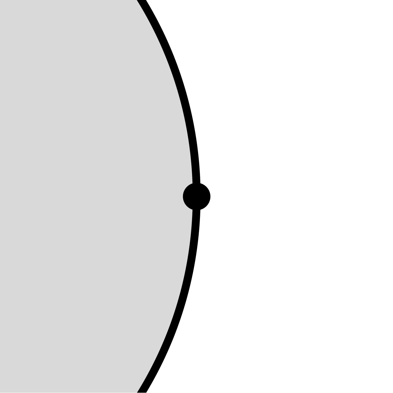
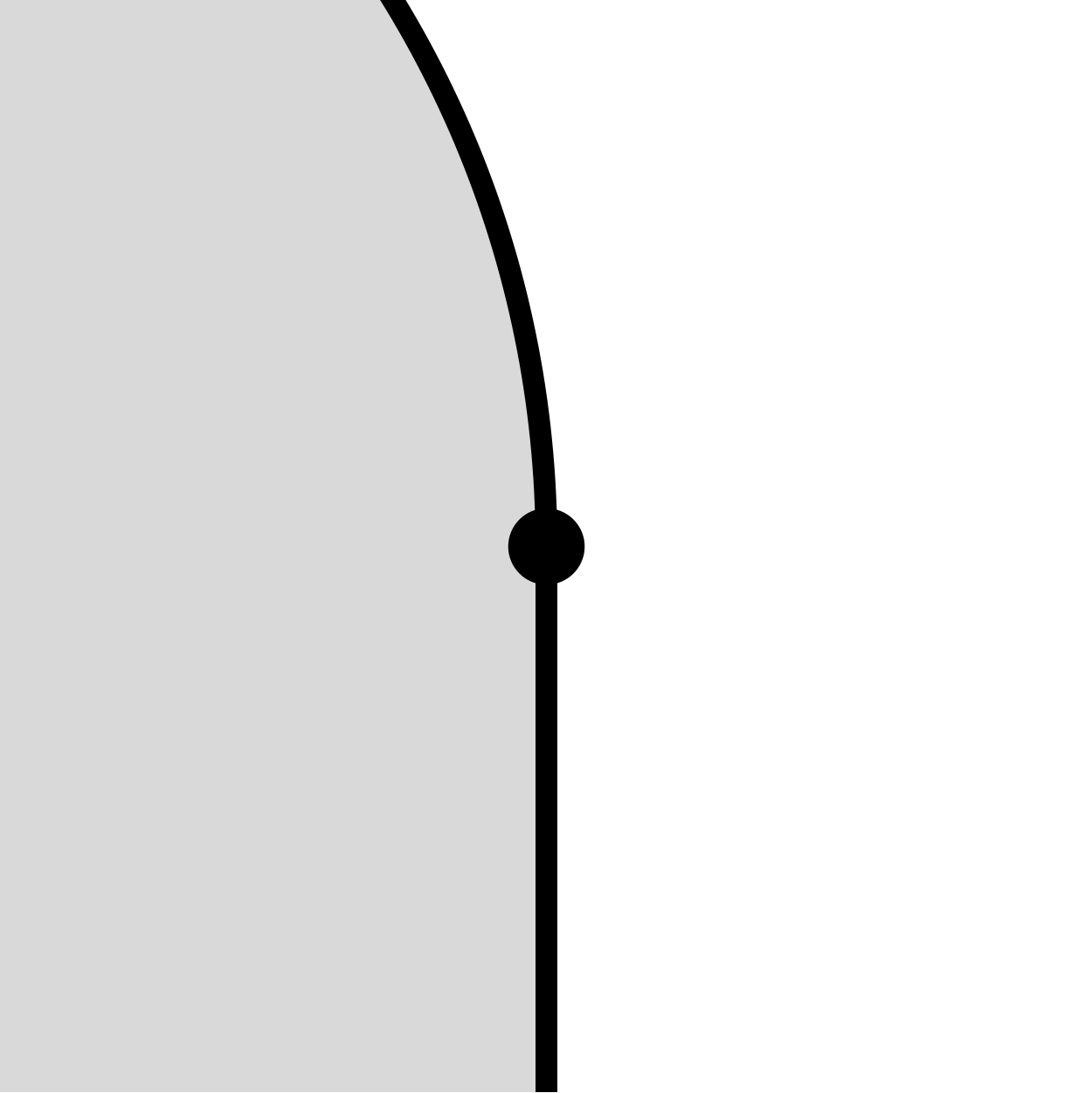
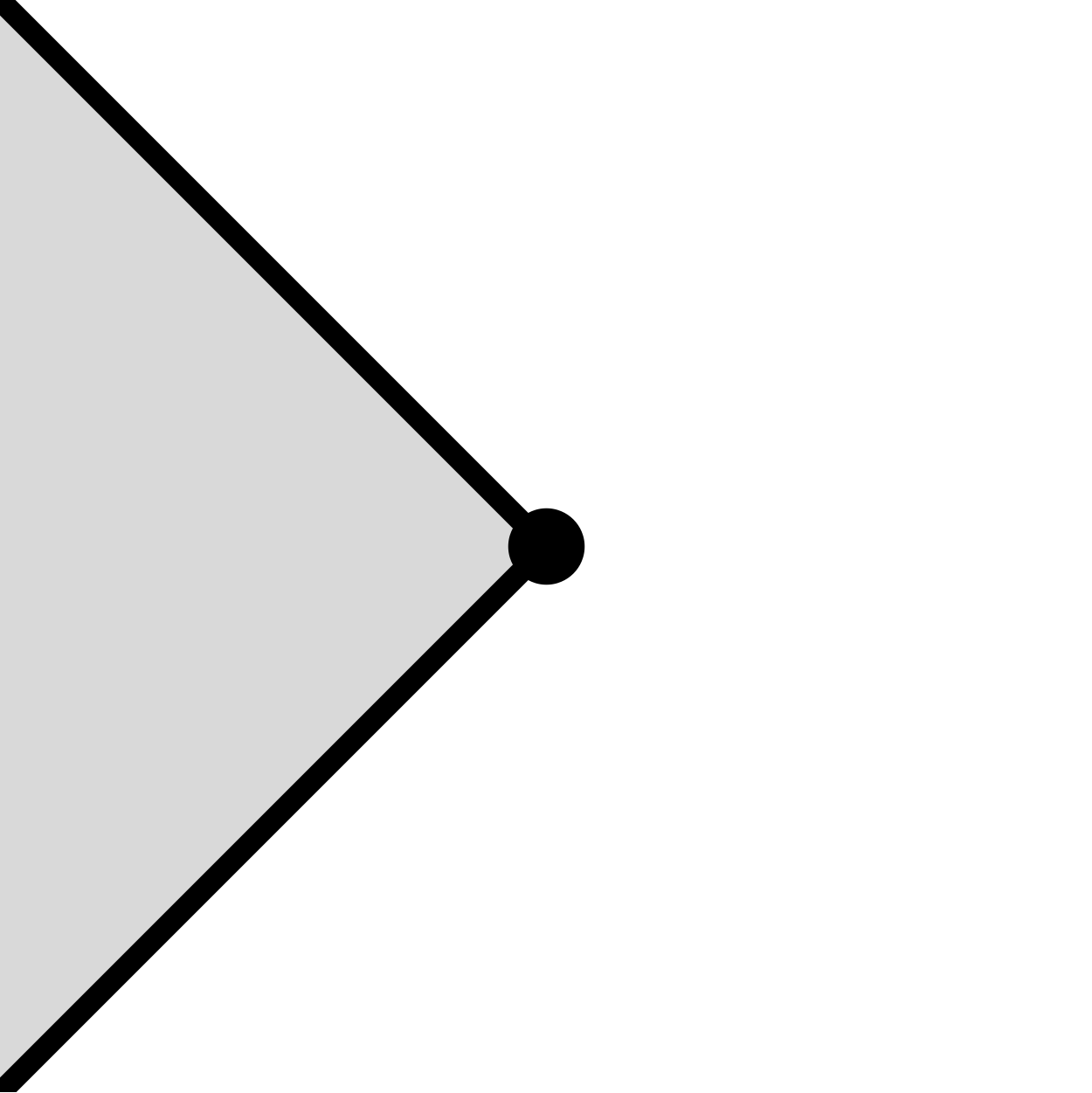
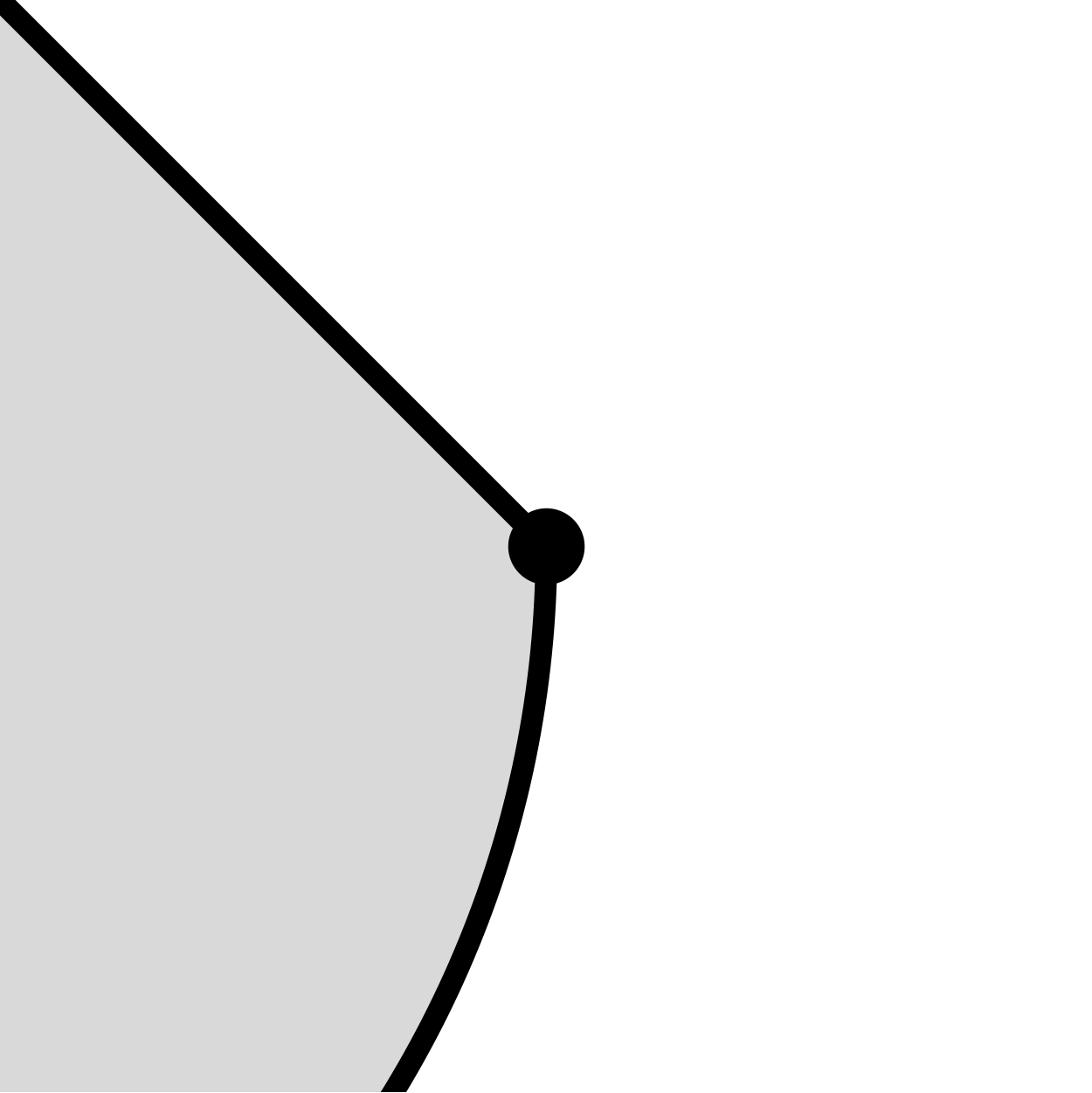
a) b) c) d) e)

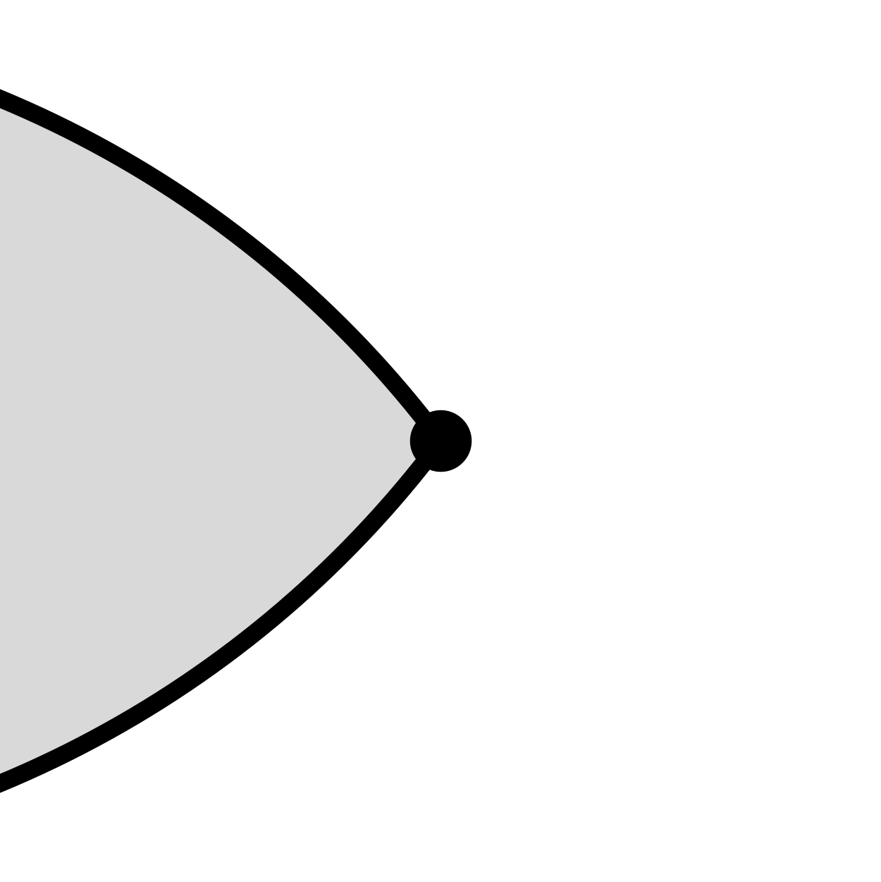
Figure 1. Extreme points of planar two-dimensional convex bodies. Regular extreme points: a) regular exposed point, b) non-exposed point. Corner points incident with c) two, d) one, or e) no facet(s).

A classification of extreme points of $K$, in terms of smoothness and flatness, is easy to state. Every singular extreme point of $K$ is a corner point and hence an exposed point. Every regular extreme point $z$ of $K$ lies on at most one facet of $K$. Otherwise $z$ would be an intersection of two facets. The antitone lattice isomorphism between exposed faces and normal cones [74] then shows that $z$ is a singular boundary point, which is a contradiction. It follows from the definitions that a regular extreme point $z$ is an exposed point if and only if $z$ lies on no facet. Figure 1 shows all possible cases.

	exposed	regular	# incident facets
regular exposed point	yes	yes	$0$
non-exposed point	no	yes	$1$
corner point	yes	no	$2$

Table 1. Extreme points of two-dimensional numerical ranges. The cases a)–c) of Figure 1 are possible, but d) and e) are inconsistent with Theorem 2.1.

If $K$ is the numerical range $W=W_{A}$ of a matrix $A\in M_{d}$, then a theorem by Donoghue [22] affirms that every corner point $z$ of $W$ is an eigenvalue of $A$. In particular, $W$ has at most finitely many corner points. The reason is that no non-degenerate ellipse included in $W$ can pass through $z$. As observed in [53], a closer look at Donoghue’s proof shows that $z$ is indeed a normal splitting eigenvalue of $A$, that is there is a non-zero $x\in\mathbb{C}^{d}$ such that $Ax=zx$ and $A^{*}x=\bar{z}x$ hold. This gives an orthogonal direct sum decomposition $A=(z)\oplus B$ where $B\in M_{d-1}$ (we ignore the unitary conjugation which brings $A$ into this form). Since $W_{A}$ is the convex hull of $z$ and $W_{B}$, either $z\not\in W_{B}$ or an analogue decomposition applies to $B$. Inductively, $W$ is the convex hull of $z$ and $W_{C}$ for some matrix $C$ with $z\not\in W_{C}$. Thus $z$ is incident with two facets of $W$. This proves the following statement.

Theorem 2.1.

Let $\dim W=2$ and let $z$ be a corner point of $W$. Then $z$ is the intersection of two facets of $W$.

Theorem 2.1 is well-known [7]. Table 1 lists the resulting classification of extreme points.

Let us now characterize regular extreme points, that is cases a) and b) of Table 1. A point $z\in K$ is a round boundary point of $K$ if $z\in\partial K$ and for all $\epsilon>0$ at least one of the one-sided $\epsilon$-neighborhoods of $z$ in $\partial K$ is not a line segment [21, 45].

Lemma 2.2.

Let $K\subset\mathbb{R}^{2}$ be a convex body, $\dim K=2$, and let $z\in\partial K$. Then we have $(1)\iff(2)\implies(3)\iff(4)$. If $K=W$ then also $(3)\implies(2)$.

1. $z\in\operatorname{reg-ext}(K)$,

2. $z$ is not a corner point of $K$ and not a relative interior point of a facet of $K$,

3. $z$ is an extreme point of $K$ which is incident with at most one facet of $K$,

4. $z$ is a round boundary point of $K$.

Proof: (1)$\iff$(2) is proved in the paragraph of (2.1). For (1)$\implies$(3) we refer to one paragraph after (2.1), see also Figure 1. We prove (3)$\implies$(4) by contradiction: If $z$ is an extreme point whose two one-sided neighborhoods are segments then these segments can be extended to two facets. (4)$\implies$(3) is easy to prove indirectly. If $K=W$ is the numerical range then (3)$\implies$(1) follows indirectly because corner points lie on two facets, see the second paragraph above this lemma. $\square$

The statement (1) respectively (2) of Lemma 2.2 is the definition of round boundary point in [44, 60, 49], respectively [68]. A stronger definition than round boundary point appears in [45]: A point $z\in K$ is a fully round boundary point of $K$, if $z\in\partial K$ and for all $\epsilon>0$ both one-sided $\epsilon$-neighborhoods of $z$ in $\partial K$ are no line segments.

Lemma 2.3.

Let $K\subset\mathbb{R}^{2}$ be a convex body, $\dim K=2$, and let $z\in\partial K$. Then we have $(1)\iff(2)\implies(3)\iff(4)$. If $K=W$ then also $(3)\implies(2)$.

1. $z\in\operatorname{reg-exp}(K)$,

2. $z$ is not a corner point of $K$, not a non-exposed point of $K$, and not a relative interior point of a facet of $K$,

3. $z$ is an extreme point of $K$ which is not incident with any facet of $K$,

4. $z$ is a fully round boundary point of $K$.

Proof: The proof is analogous to the proof of Lemma 2.2. $\square$

Outside of the corner points, the geometry of $\partial W$ is characterized by its curvature. Let $z\in\operatorname{reg}(K)$, that is $z$ is a smooth boundary point. Choose the cartesian coordinate system of $\mathbb{R}^{2}$ such that $z=(0,0)$ and $K\subset\{(\xi,\eta)\in\mathbb{R}:\eta\geq 0\}$ (orthogonal coordinates in standard orientation). Then there is $\epsilon>0$ and a convex function $f:\,]-\epsilon,\epsilon[\to\mathbb{R}$ such that $\xi\mapsto(\xi,f(\xi))$ parametrizes $\partial K$ locally around $z$. Recall that $f^{\prime}(0)=0$ holds, for example see Section 2 of [13] or Theorem 1.5.4 of [63].

We distinguish a counterclockwise one-sided neighborhood of $z\in\partial K$, which extends from $z$ in counterclockwise direction along $\partial K$, from a clockwise neighborhood which extends in clockwise direction. Using the notation from the preceding paragraph, we define the counterclockwise respectively clockwise curvature of $\partial K$ at $z$ by

(2.2) $$\kappa_{+}(z):=\lim_{\xi\searrow 0}\frac{2f(\xi)}{\xi^{2}}\qquad\mbox{respectively}\quad\kappa_{-}(z):=\lim_{\xi\nearrow 0}\frac{2f(\xi)}{\xi^{2}},$$

if the limit exists. The one-sided radii of curvature of $\partial K$ at $z$ are $\rho_{\pm}(z):=1/\kappa_{\pm}(z)$. To connect to the literature, we define the upper respectively lower curvature of $\partial K$ at $z$ to be

(2.3) $$\kappa_{s}(z):=\limsup_{\xi\to 0}\frac{2f(\xi)}{\xi^{2}}\quad\mbox{respectively}\quad\kappa_{i}(z):=\liminf_{\xi\to 0}\frac{2f(\xi)}{\xi^{2}}.$$

If $\kappa_{s}(z)=\kappa_{i}(z)$ then $\kappa(z):=\kappa_{s}(z)$ is the curvature and $\rho(z):=1/\kappa(z)$ the radius of curvature of $\partial K$ at $z$, including possible values of $\{0,+\infty\}$.

An explicit formula for $\rho(z)$ is known [25] for the numerical range $W$ in terms of matrix entries of $A$, see also [14]. Notice that if $f$ is twice differentiable at $0$, then $\kappa(z)=f^{\prime\prime}(0)$ holds because (2.2) denotes the second right and left de la Vall e-Poussin derivatives of $f$ at $0$, see Section 2 of [13]. If $f$ is $C^{2}$ at $0$ and $f^{\prime\prime}(0)>0$ then $\rho(z)=1/f^{\prime\prime}(0)$ is the radius of the osculating circle of $\partial K$ at $z$, see for example [69]. If $f$ is not $C^{2}$ at $0$, then $\rho(z)=0$ may happen. An example is $f(\xi)=\xi^{\alpha}$ with $1<\alpha<2$. For $K=W$ the numerical range, this is known to be impossible [51].

Theorem 2.4 (Marcus and Filippenko).

Let $z$ be a regular boundary point of $W$. Then $\kappa_{s}(z)<\infty$.

Proof: If the upper curvature $\kappa_{s}(z)=\infty$ is infinite, then no non-degenerate ellipse included in $W$ can pass through $z$. As explained in the paragraph above Theorem 2.1, in that case $z$ is a corner point of $W$. $\square$

More recently, a discussion of infinite curvature of the boundary of the numerical range of a bounded operator on a Hilbert space took place. It was conjectured [32] that all regular boundary points of the numerical range with infinite lower curvature belong to the essential spectrum of that operator. This conjecture was proved independently in the articles [24, 62, 67]. The corresponding stronger result about infinite upper curvature was proved in [30] and gives an alternative proof of Theorem 2.4, because there is no essential spectrum in finite dimensions.

3. Differential geometry of planar convex bodies

We study two maps $x_{K,\pm}$ from the unit circle $S^{1}$ to the extreme points of a planar convex body $K$. If the values of $x_{K,\pm}$ agree at a normal vector then they agree with the reverse Gauss map $x_{K}$. Otherwise $x_{K}$ is undefined and $x_{K,\pm}$ describe pairs of distinct extreme points of boundary segments. The image of $x_{K}$ intersected with the regular boundary points is the set of regular exposed points $\operatorname{reg-exp}(K)$ whose differential geometry will be the focus of this section, along with limit points of the set $\operatorname{reg-exp}(K)$. Since the differentiability order of $x_{K}$ is too small for our purposes we will also study a dual convex body $K^{*}$.

Let $K\subset\mathbb{R}^{2}$ be a convex body. The support function of $K$ is

$${\bf h}_{K}:\mathbb{R}^{2}\to\mathbb{R},\qquad u\mapsto\min_{x\in K}\langle x,u\rangle.$$

The function ${\bf h}_{K}$ is concave, continuous, and positively homogenous [63]. Non-empty exposed faces of $K$ are parametrized in terms of their inner normal vectors by

$$F_{K}:\mathbb{R}^{2}\to 2^{K},\qquad u\mapsto\operatorname*{argmin}_{x\in K}\langle x,u\rangle,$$

where $2^{K}$ denotes the set of subsets of $K$. If $u$ is a unit vector then $F_{K}(u)$ is a singleton or a closed segment and we can denote its extreme point(s) by $x_{K,+}(u)$ and $x_{K,-}(u)$. Formally, we define two maps $x_{K,+}$ and $x_{K,-}$ by

$$x_{K,\pm}:S^{1}\to\partial K,\qquad u\mapsto u\cdot[{\bf h}_{K}(u)\pm\operatorname{i}{\bf h}_{F_{K}(u)}(\pm\operatorname{i}u)].$$

The union of the images of $x_{K,\pm}$ is the set of extreme points of $K$. Indeed, $x_{K,\pm}(u)$ is an extreme point of $K$ since it is an extreme point of $F_{K}(u)$. Conversely, every non-exposed point of $K$ is an exposed point of a facet of $K$, see Figure 1 b), and see [68] for more details. For all extreme points $z$ of $K$ and unit vectors $u\in S^{1}$, a general property of normal vectors and exposed faces [74], applied to the exposed face $F_{K}(u)$, proves that

(3.1) $$z=x_{K,\pm}(u)\iff\mbox{$u$ is an inner normal vector of $K$ at $z$}.$$

Thereby $z=x_{K,\pm}(u)$ stands for $z=x_{K,+}(u)$ or $z=x_{K,-}(u)$, but not necessarily for both. In the following the meaning of the $\pm$-symbol will be clear from the context.

A unit vector $u\in S^{1}$ is a regular normal vector [63] of $K$ if $x_{K,+}(u)=x_{K,-}(u)$ holds, that is, if $F_{K}(u)$ is a singleton. Otherwise we call $u$ a singular normal vector. Let $\operatorname{regn}(K)$ denote the set of regular normal vectors of $K$, and let

$$\Xi_{K}:=\{\theta\in\mathbb{R}:e^{\operatorname{i}\theta}\in\operatorname{regn}(K)\}$$

be its angular representation. The reverse Gauss map is defined by

$$x_{K}:\operatorname{regn}(K)\to\partial K,\qquad\{x_{K}(u)\}=F_{K}(u).$$

The Gauss map is the function

$$u_{K}:\operatorname{reg}(K)\to S^{1}$$

such that $u_{K}(x)$ is the unique inner unit normal vector of $K$ at $x\in\operatorname{reg}(K)$.

Figure 2. Commutative diagram for the Gauss map $u_{K}$ and reverse Gauss map $x_{K}$ of a planar convex body $K$ with angular parametrizations. Hooked arrows denote embeddings.

Notice that the image of $x_{K}$ is the set of exposed points of $K$. Its intersection with the domain of $u_{K}$ is the set $\operatorname{reg-exp}(K)$ of regular exposed points of $K$. Both the Gauss map $u_{K}$ and the reverse Gauss map $x_{K}$ are continuous, see for example Section 2.2 of [63]. The restriction of $u_{K}$ to $\operatorname{reg-exp}(K)$ is a homeomorphism onto

(3.2) $$\operatorname{un-regn}(K):=\{u_{K}(x):x\in\operatorname{reg-exp}(K)\}.$$

The inverse homeomorphism is the restriction of $x_{K}$ to $\operatorname{un-regn}(K)$. The set of angles corresponding to $\operatorname{un-regn}(K)$ is

$$\Xi_{K}^{R}:=\{\theta\in\mathbb{R}:e^{\operatorname{i}\theta}\in\operatorname{un-regn}(K)\}.$$

A summary of Gauss map, reverse Gauss map, and their natural restrictions is given in Figure 2.

Although ${\bf h}_{K}$ may not be differentiable, its directional derivatives do exist. The directional derivative of $f:\mathbb{R}^{k}\to\mathbb{R}$ at $u\in\mathbb{R}^{k}$ in the direction of $v\in\mathbb{R}^{k}$ is

$$f^{\prime}(u;v):=\lim_{\begin{subarray}{c}t\searrow 0\end{subarray}}[f(u+tv)-f(u)]/t,$$

if the limit exists. For $u,v\in\mathbb{R}^{2}$ we have ${\bf h}_{F_{K}(u)}(v)={\bf h}^{\prime}_{K}(u;v)$, see for example Theorem 1.7.2 of [63] or Section 16 of [11]. In particular,

$${\bf h}_{F_{K}(u)}(\pm\operatorname{i}u)={\bf h}_{K}^{\prime}(u;\pm\operatorname{i}u),\qquad u\in S^{1},$$

which shows

(3.3) $$x_{K,\pm}(u)=u\cdot[{\bf h}_{K}(u)\pm\operatorname{i}{\bf h}_{K}^{\prime}(u;\pm\operatorname{i}u)],\qquad u\in S^{1}.$$

Let $h_{K}(\theta):={\bf h}_{K}(e^{\operatorname{i}\theta})$, $\theta\in\mathbb{R}$. An easy calculation, see for example Lemma 2.2 of [68], shows

(3.4) $$h_{K}^{\prime}(\theta;\pm 1)={\bf h}_{K}^{\prime}(e^{\operatorname{i}\theta};\pm\operatorname{i}e^{\operatorname{i}\theta}),\qquad\theta\in\mathbb{R}.$$

One obtains

(3.5) $$x_{K,\pm}(e^{\operatorname{i}\theta})=e^{\operatorname{i}\theta}\cdot[h_{K}(\theta)\pm\operatorname{i}h_{K}^{\prime}(\theta;\pm 1)]$$

from the preceding equations (3.3) and (3.4).

First order differentiability of ${\bf h}_{K}$ is perfectly understood. Since ${\bf h}_{K}$ is positively homogeneous, we have for $r>0$ and $\theta\in\mathbb{R}$

$$\textstyle\frac{\partial}{\partial r}{\bf h}_{K}(re^{\operatorname{i}\theta})={\bf h}_{K}(e^{\operatorname{i}\theta})=h_{K}(\theta).$$

For all $\theta\in\Xi_{K}$ we get from (3.4)

$$\textstyle\frac{\partial}{\partial\theta}{\bf h}_{K}(re^{\operatorname{i}\theta})=r\frac{\partial}{\partial\theta}{\bf h}_{K}(e^{\operatorname{i}\theta})=rh_{K}^{\prime}(\theta).$$

Hence, ${\bf h}_{K}$ is differentiable on open subsets of $\{ru:r>0,u\in\operatorname{regn}(K)\}$ and the gradient is

(3.6) $$\nabla{\bf h}_{K}(re^{\operatorname{i}\theta})=e^{\operatorname{i}\theta}[h_{K}(\theta)+\operatorname{i}h_{K}^{\prime}(\theta)],\qquad r>0,\theta\in\Xi_{K}.$$

The equations (3.5) and (3.6) show

(3.7) $$x_{K}(e^{\operatorname{i}\theta})=e^{\operatorname{i}\theta}[h_{K}(\theta)+\operatorname{i}h_{K}^{\prime}(\theta)]=\nabla{\bf h}_{K}(e^{\operatorname{i}\theta}),\qquad\theta\in\Xi_{K}.$$

Since $x_{K}$ is continuous, ${\bf h}_{K}$ is a $C^{1}$-map on open subsets of $\{ru:r>0,u\in\operatorname{regn}(K)\}$, and $h_{K}$ is a $C^{1}$-map on open subsets of $\Xi_{K}$.

Second derivatives of ${\bf h}_{K}$ are needed to address first derivatives of $x_{K}$ and radii of curvature of $\partial W$. Let $\Xi^{(2)}_{K}\subset\Xi_{K}$ denote the largest open set in $\mathbb{R}$ on which $h_{K}$ is twice continuously differentiable. It follows from (3.6) that for all $r>0$ and $\theta\in\Xi^{(2)}_{K}$ the Jacobian of $\nabla{\bf h}_{K}$ at $re^{\operatorname{i}\theta}$ with respect to the orthonormal basis $\{e^{\operatorname{i}\theta},\operatorname{i}e^{\operatorname{i}\theta}\}$ is

$$\nabla{\bf h}_{K}(re^{\operatorname{i}\theta})=\frac{1}{r}\left(\begin{array}[]{cc}0&0\\ 0&h_{K}(\theta)+h_{K}^{\prime\prime}(\theta)\end{array}\right).$$

This shows that ${\bf h}_{K}$ is a $C^{2}$-map on the open set $\{re^{\operatorname{i}\theta}:r>0,\theta\in\Xi^{(2)}_{K}\}$. Since ${\bf h}_{K}$ is concave, the above matrix is negative semi-definite. This shows

(3.8) $$h_{K}(\theta)+h_{K}^{\prime\prime}(\theta)\leq 0,\qquad\theta\in\Xi^{(2)}_{K}.$$

Moreover, (3.7) shows that $x_{K}$ is a $C^{1}$-map on $\{e^{\operatorname{i}\theta}:\theta\in\Xi^{(2)}_{K}\}\subset S^{1}$, whose differential

(3.9) $$({\rm d}x_{K})_{e^{\operatorname{i}\theta}}(\operatorname{i}e^{\operatorname{i}\theta})=\operatorname{i}e^{\operatorname{i}\theta}\cdot[h_{K}(\theta)+h_{K}^{\prime\prime}(\theta)],\qquad\theta\in\Xi^{(2)}_{K},$$

is defined on the tangent space of $S^{1}$ at $e^{\operatorname{i}\theta}$. The differential $({\rm d}x_{K})_{e^{\operatorname{i}\theta}}$ is known as the reverse Weingarten map [63]. Its eigenvalue is $h_{K}(\theta)+h_{K}^{\prime\prime}(\theta)$. The non-negative number $-h_{K}(\theta)-h_{K}^{\prime\prime}(\theta)$ is the radius of curvature of $\partial K$ at $x_{K}(e^{\operatorname{i}\theta})$, see for example Section 39 of [11]. More generally, the one-sided radii of curvature, defined in the paragraph of (2.2), are as follows.

Lemma 3.1 (Radii of curvature).

Let $z\in\operatorname{reg}(K)$ and let $]\varphi_{1},\varphi_{2}[\,\subset\Xi^{(2)}_{K}$ be an open interval on which $h_{K}+h_{K}^{\prime\prime}$ is strictly negative. If $z=\lim_{\theta\searrow\varphi_{1}}x_{K}(e^{\operatorname{i}\theta})$ respectively $z=\lim_{\theta\nearrow\varphi_{2}}x_{K}(e^{\operatorname{i}\theta})$ then

$$\rho_{+}(z)=-\lim_{\theta\searrow\varphi_{1}}[h_{K}(\theta)+h_{K}^{\prime\prime}(\theta)],\qquad\mbox{respectively}\qquad\rho_{-}(z)=-\lim_{\theta\nearrow\varphi_{2}}[h_{K}(\theta)+h_{K}^{\prime\prime}(\theta)].$$

Proof: Without loss of generality let $\varphi_{1}=0$ and assume $z=\lim_{\theta\searrow 0}x_{K}(e^{\operatorname{i}\theta})$. Notice that $x_{K}(1)$ lies on the vertical supporting line to the left of $K$ and that the curve $x_{K}(e^{\operatorname{i}\theta})$, $\theta\in\,]0,\varphi_{2}[$, parametrizes an arc of $\partial K$ which extends counterclockwise from $z$ along $\partial K$. The latter follows also from by (3.21). The coordinates of $x_{K}(e^{\operatorname{i}\theta})$, introduced in the paragraph preceding (2.2), are

$$(\xi,\eta)=[-\operatorname{Im}\,v(\theta),\operatorname{Re}\,v(\theta)],$$

where $v(\theta):=x_{K}(e^{\operatorname{i}\theta})-z$. We recall from (3.9) that $v^{\prime}(\theta)=\operatorname{i}e^{\operatorname{i}\theta}f(\theta)$ holds, where we abbreviate $f(\theta):=h_{K}(\theta)+h_{K}^{\prime\prime}(\theta)$. By the assumption $f(\theta)<0$ we have

$$\operatorname{Re}(v(\theta))^{\prime}=\operatorname{Re}(v^{\prime}(\theta))=-\operatorname{Im}(e^{\operatorname{i}\theta})f(\theta)=-\sin(\theta)f(\theta)\neq 0.$$

Twice applying l’H pital’s rule then gives

$$\rho_{+}(z)=\lim_{\theta\searrow 0}\frac{\operatorname{Im}(v(\theta))^{2}}{2\operatorname{Re}(v(\theta))}=\lim_{\theta\searrow 0}\frac{\operatorname{Im}(v(\theta))\cos(\theta)}{-\sin(\theta)}=-\lim_{\theta\searrow 0}f(\theta).$$

The proof for the clockwise radius of curvature is analogous. $\square$

Our next aim is to relate the differentiability of $\operatorname{reg-exp}(K)\subset\partial K$ as a submanifold of $\mathbb{C}$ and the differentiability of $h_{K}$ as a function. Our proof is a generalization of two passages from pages 115 and 120 in Section 2.5 of [63], where the analogous statements are proved globally. Notice from Lemma 3.1 that radii of curvature depend on the support function. Thus the statements of Lemma 3.2 and Theorem 3.3 distinguish conceptually between $\partial K$ as a manifold and $h_{K}$ as a function.

Lemma 3.2.

Let $z\in\operatorname{reg-exp}(K)$ and $\theta\in\Xi_{K}^{R}$ be such that $z=x_{K}(e^{\operatorname{i}\theta})$, and let $k\geq 2$. If $\operatorname{reg-exp}(K)$ is locally at $z$ a $C^{k}$-submanifold of $\mathbb{C}$ and $u_{K}$ is locally at $z$ a $C^{k-1}$-diffeomorphism, then $h_{K}$ is locally at $\theta$ of class $C^{k}$ and the radius of curvature of $\partial K$ is finite and strictly positive at $z$.

Proof: Let $M\subset\operatorname{reg-exp}(K)$ be a $C^{k}$-submanifold of $\mathbb{C}$ such that $U:=u_{K}(M)$ is an open arc segment of $S^{1}$ and let $z\in M$. The support function is

(3.10) $${\bf h}_{K}(u)=\langle x_{K}(u),u\rangle,\qquad u\in U,$$

because $U\subset\operatorname{regn}(K)$. By assumption, $u_{K}$ is a $C^{k-1}$-diffeomorphism on $M$. Hence the inverse $x_{K}$, defined on $U$, is of class $C^{k-1}$. Now (3.10) shows that ${\bf h}_{K}$ is of class $C^{k-1}$ on $\{ru:r>0,u\in U\}$. In particular ${\bf h}_{K}$ is differentiable, so (3.7) proves

$$\nabla{\bf h}_{K}(u)=x_{K}(u),\qquad u\in U.$$

This shows that ${\bf h}_{K}$ is of class $C^{k}$ in a neighborhood of $u_{K}(z)$, so that $h_{K}$ is of class $C^{k}$ in a neighborhood of $\theta$. For $e^{\operatorname{i}\theta}\in U$ the eigenvalue of the differential $({\rm d}x_{K})_{e^{\operatorname{i}\theta}}$ is $h_{K}(\theta)+h_{K}^{\prime\prime}(\theta)<0$ by (3.9) and (3.8), since $x_{K}$ is a diffeomorphism on $U$. Lemma 3.1 shows that the radius of curvature of $M$ at $z$ is $-h_{K}(\theta)-h_{K}^{\prime\prime}(\theta)>0$. $\square$

To prove the converse of Lemma 3.2, let us assume without loss of generality that $0\in\mathbb{C}$ is an interior point of $K$. This is justified because the support function transforms under a translation by a vector $v\in\mathbb{C}$ into ${\bf h}_{K+v}={\bf h}_{K}+{\bf h}_{v}$ where ${\bf h}_{v}$ is linear. The dual of $K$,

$$K^{*}:=\{u\in\mathbb{C}:1+\langle u,z\rangle\geq 0,z\in K\},$$

is a convex body with $0$ in its interior, and $(K^{*})^{*}=K$ holds. For every convex subset $F\subset K$ the set

$$\mathcal{C}_{K}(F):=\{u\in K^{*}:1+\langle u,z\rangle=0,z\in F\}$$

is an exposed face of $K^{*}$. We call $\mathcal{C}_{K}(F)$ the dual face of $F$. Let us also define the normal cone of $K$ at $F$ by

$$N_{K}(F):=\{u\in\mathbb{C}:\langle u,y-z\rangle\geq 0,y\in K,z\in F\}.$$

We write $N_{K}(z):=N_{K}(\{z\})$ and $\mathcal{C}_{K}(z):=\mathcal{C}_{K}(\{z\})$ for $z\in K$. The positive hull of a non-empty subset $U\subset\mathbb{C}$ is ${\rm pos}\,U:=\{ru:u\in U,r\geq 0\}$ while ${\rm pos}\,\emptyset:=\{0\}$ by convention.

For completeness, we prove that the conjugate face of $z\in\operatorname{reg-exp}\,K$ is the regular exposed point of $K^{*}$ obtained by positive scaling of the inner unit normal vector of $K$ at $z$. Moreover, the induced map (3.16) is a bijection. To begin with, we recall that $\mathcal{C}_{K^{*}}[\mathcal{C}_{K}(F)]$ is the smallest exposed face of $K$ containing a convex subset $F\subset K$. Further, we have

(3.11) $$N_{K}(F)={\rm pos}[\mathcal{C}_{K}(F)],$$

see for example Lemma 2.2.3 of [63].

Let us first exploit (3.11) for a regular boundary point $z\in\operatorname{reg}\,K$. The normal cone $N_{K}(z)$ is a ray, $\mathcal{C}_{K}(z)$ is an exposed point of $K^{*}$, and an easy calculation shows $\mathcal{C}_{K}(z)=x_{K^{*}}(z/|z|)$. By choosing unit vectors in the equality of rays (3.11), one has

(3.12) $$u_{K}(z)=x_{K^{*}}(\tfrac{z}{|z|})/|x_{K^{*}}(\tfrac{z}{|z|})|,\qquad z\in\operatorname{reg}(K).$$

The radial function of $K$ is

$${\bf r}_{K}:\mathbb{R}^{2}\setminus\{0\}\to\mathbb{R},\quad u\mapsto\max\{r\geq 0:r\cdot u\in K\}.$$

Using the radial function of $K^{*}$ and (3.12) we obtain for $z\in\operatorname{reg}(K)$

(3.13) $$x_{K^{*}}(z/|z|)=u_{K}(z)\cdot{\bf r}_{K^{*}}(u_{K}(z)).$$

For later reference, we notice [63]

(3.14) $${\bf r}_{K^{*}}(u)=-{\bf h}_{K}(u)^{-1},\qquad u\in\mathbb{R}^{2}\setminus\{0\}.$$

Replacing $K$ with $K^{*}$, equation (3.12) becomes

(3.15) $$u_{K^{*}}(u)=x_{K}(\tfrac{u}{|u|})/|x_{K}(\tfrac{u}{|u|})|,\qquad u\in\operatorname{reg}(K^{*}).$$

As pointed out above, $\mathcal{C}_{K}(z)=x_{K^{*}}(z/|z|)$ is an exposed point. If the point $z$ is an exposed point then (3.11) and $\mathcal{C}_{K^{*}}[\mathcal{C}_{K}(z)]=z$ show that $N_{K^{*}}(\mathcal{C}_{K}(z))={\rm pos}(z)$. So $\mathcal{C}_{K}(\operatorname{reg-exp}K)\subset\operatorname{reg-exp}(K^{*})$ follows. Replacing $K$ with $K^{*}$ we obtain that

(3.16) $$\mathcal{C}_{K}|_{\operatorname{reg-exp}(K)}:\operatorname{reg-exp}(K)\to\operatorname{reg-exp}(K^{*}),\qquad z\mapsto x_{K^{*}}(z/|z|),$$

is a bijection.

Theorem 3.3.

Let $z\in\operatorname{reg-exp}(K)$ and $\theta\in\Xi_{K}^{R}$ be such that $z=x_{K}(e^{\operatorname{i}\theta})$, and let $k\geq 2$. The set $\operatorname{reg-exp}(K)$ is locally at $z$ a $C^{k}$-submanifold of $\mathbb{C}$ and $u_{K}$ is locally at $z$ a $C^{k-1}$-diffeomorphism if and only if $h_{K}$ is locally at $\theta$ of class $C^{k}$ and the radius of curvature of $\partial K$ is finite and strictly positive at $z$.

Proof: Let $h_{K}$ be locally at $\theta$ of class $C^{k}$ and let the radius of curvature of $\partial K$ at $z=x_{K}(e^{\operatorname{i}\theta})$ be strictly positive. In the next two paragraphs we show that $\partial K^{*}$ is locally at $\mathcal{C}_{K}(z)$ a $C^{k}$-submanifold of $\mathbb{C}$ and that $u_{K^{*}}$ is locally at $\mathcal{C}_{K}(z)$ a $C^{k-1}$-diffeomorphism. Assuming that, Lemma 3.2 shows that the radius of curvature of $\partial K^{*}$ is strictly positive at $z^{*}:=\mathcal{C}_{K}(z)$ and that $h_{K^{*}}$ is locally at $\theta^{*}$ of class $C^{k}$ where $\theta^{*}\in\Xi_{K^{*}}^{R}$ is such that $z^{*}=x_{K^{*}}(e^{\operatorname{i}\theta^{*}})$. The next two paragraphs, when $K,z,\theta$ is replaced with $K^{*},z^{*},\theta^{*}$, show that $\operatorname{reg-exp}(K)$ is locally at

$$\mathcal{C}_{K^{*}}(z^{*})=\mathcal{C}_{K^{*}}[\mathcal{C}_{K}(z)]=z$$

a $C^{k}$-submanifold of $\mathbb{C}$ and that $u_{K}$ is locally at $z$ a $C^{k-1}$-diffeomorphism. The proof is completed by Lemma 3.2.

We assume that $0$ is an interior point of $K$ and show that $\operatorname{reg-exp}(K^{*})$ is locally at $\mathcal{C}_{K}(z)$ a $C^{k}$-submanifold of $\mathbb{C}$. The map $\mathcal{C}_{K}\circ x_{K}:\operatorname{un-regn}(K)\to\operatorname{reg-exp}(K^{*})$ to the dual convex body has by (3.2), (3.16), and (3.13) the form

(3.17) $$\operatorname{un-regn}(K)\to\operatorname{reg-exp}(K^{*}),\qquad u\mapsto u\cdot{\bf r}_{K^{*}}(u).$$

We study (3.17) in angular coordinates, described in Figure 2, where the map takes the form

(3.18) $$\Xi_{K}^{R}\to\operatorname{reg-exp}(K^{*}),\qquad\varphi\mapsto e^{\operatorname{i}\varphi}\cdot{\bf r}_{K^{*}}(e^{\operatorname{i}\varphi}).$$

Using (3.14), we have

$$e^{\operatorname{i}\varphi}\cdot{\bf r}_{K^{*}}(e^{\operatorname{i}\varphi})=-e^{\operatorname{i}\varphi}/{\bf h}_{K}(e^{\operatorname{i}\varphi})=-e^{\operatorname{i}\varphi}/h_{K}(\varphi).$$

Since $h_{K}$ is assumed to be at $\theta$ of class $C^{k}$, it follows that (3.17) is locally at $e^{\operatorname{i}\theta}$ of class $C^{k}$. Using (3.7), the differential of (3.18) is

$$\frac{\partial}{\partial\varphi}\left(-\frac{e^{\operatorname{i}\varphi}}{h_{K}(\varphi)}\right)=\frac{x_{K}(e^{\operatorname{i}\varphi})}{\operatorname{i}h_{K}(\varphi)^{2}},$$

which is non-zero because $0$ is an interior point of $K$. Hence, the map (3.17) is locally at $e^{\operatorname{i}\theta}$ a diffeomorphism. Since the inverse of (3.17) is continuous by a Theorem of Sz. Nagy [10], this proves that $\partial K^{*}$ is locally at $\mathcal{C}_{K}(z)=e^{\operatorname{i}\theta}\cdot{\bf r}_{K^{*}}(e^{\operatorname{i}\theta})$ a $C^{k}$-submanifold of $\mathbb{C}$, see for example Section 3.1 of [1].

Let us prove that $u_{K^{*}}$ is locally at $\mathcal{C}_{K}(z)$ a diffeomorphism. The reverse Gauss map $x_{K}$ is locally at $e^{\operatorname{i}\theta}$ of class $C^{k-1}$, since $x_{K}(e^{\operatorname{i}\varphi})=\nabla{\bf h}_{K}(e^{\operatorname{i}\varphi})$ holds by (3.7). The eigenvalue of $({\rm d}x_{K})_{e^{\operatorname{i}\theta}}$ is minus the radius of curvature of $\partial K$ at $z=x_{K}(e^{\operatorname{i}\theta})$ (see (3.9) and Lemma 3.1) which is assumed to be strictly positive. Therefore $x_{K}$ is locally at $e^{\operatorname{i}\theta}$ a $C^{k-1}$-diffeomorphism. Since $\mathcal{C}_{K}(z)/|\mathcal{C}_{K}(z)|=e^{\operatorname{i}\theta}$ holds, the equation (3.15) shows that $u_{K^{*}}$ is locally at $\mathcal{C}_{K}(z)$ a composition of $C^{k-1}$-diffeomorphisms and therefore $u_{K^{*}}$ is itself locally at $\mathcal{C}_{K}(z)$ a $C^{k-1}$-diffeomorphism. $\square$

We remark that the Gauss map $u_{K}$ is a useful local chart for more general manifolds [43, 26] than the boundary of a convex body.

For completeness we discuss orientation of the reverse Gauss map of $K$. We assume that $0\in\mathbb{R}^{2}$ is an interior point of $K$, so $h_{K}(\theta)<0$ holds for all $\theta\in\mathbb{R}$. By the definition of $x_{K,\pm}$ and (3.3), the angle $\alpha_{K,\pm}(\theta)$ between the vector from $x_{K,\pm}(e^{\operatorname{i}\theta})$ to the origin $0$ and the positive real axis is

(3.19) $$\alpha_{K,\pm}(\theta)=\theta\pm\arctan\left(\tfrac{{\bf h}_{K}^{\prime}(e^{\operatorname{i}\theta};\pm\operatorname{i}e^{\operatorname{i}\theta})}{{\bf h}_{K}(e^{\operatorname{i}\theta})}\right),\qquad\theta\in\mathbb{R}.$$

Monotonicity of directional derivatives, ${\bf h}_{K}^{\prime}(e^{\operatorname{i}\theta};\operatorname{i}e^{\operatorname{i}\theta})\leq-{\bf h}_{K}^{\prime}(e^{\operatorname{i}\theta};-\operatorname{i}e^{\operatorname{i}\theta})$, see for example Theorem 1.5.4 of [63], shows that

(3.20) $$\alpha_{K,+}(\theta)-\alpha_{K,-}(\theta)\geq 0,\qquad\theta\in\mathbb{R}.$$

Equality holds in (3.20) if and only if $x_{K,+}(\theta)=x_{K,-}(\theta)$, in which case we have $x_{K}(\theta)=x_{K,\pm}(\theta)$ and we define $\alpha_{K}(\theta):=\alpha_{K,\pm}(\theta)$. Assuming $\theta\in\Xi^{(2)}_{K}\subset\Xi_{K}$, the function $h_{K}$ is twice differentiable at $\theta$. Then equations (3.19), (3.4), and (3.8) prove

(3.21) $$\alpha_{K}^{\prime}(\theta)=\tfrac{h_{K}(\theta)}{h_{K}(\theta)^{2}+h_{K}^{\prime}(\theta)^{2}}[h_{K}(\theta)+h_{K}^{\prime\prime}(\theta)]\geq 0,\qquad\theta\in\Xi^{(2)}_{K}.$$

Thereby $\alpha_{K}^{\prime}(\theta)>0$ holds if and only if $h_{K}(\theta)+h_{K}^{\prime\prime}(\theta)<0$. In other words (3.9), the orientation of $x_{K}$ is positive on open subsets of $\operatorname{regn}(K)$ where $x_{K}$ is a $C^{1}$ diffeomorphism.

4. Differential geometry of the numerical range

We study the smoothness of the boundary $\partial W$ of the numerical range in terms of the smoothness of the smallest eigenvalue $\lambda$, including their differentiability orders. The analytic differential geometry of $\partial W$ was studied earlier [29].

The support function ${\bf h}_{W}$ of $W$ at $u\in\mathbb{C}$ is the smallest eigenvalue of the hermitian matrix $\operatorname{Re}(\overline{u}A)$. For unit vectors $e^{\operatorname{i}\theta}$, as pointed out in (1.2), this means

$$h_{W}(\theta)={\bf h}_{W}(e^{\operatorname{i}\theta})=\lambda(\theta),\qquad\theta\in\mathbb{R}.$$

We will mostly work with $\lambda$ in place of $h_{W}$ or ${\bf h}_{W}$. We use an angular coordinate $\theta$ and a circular coordinate $\gamma(\theta)=e^{\operatorname{i}\theta}$.

There is [59] an analytic curve of orthonormal bases of $\mathbb{C}^{d}$,

(4.1) $$|\psi_{1}(\theta)\rangle,\ldots,|\psi_{d}(\theta)\rangle,\qquad\theta\in\mathbb{R},$$

consisting of eigenvectors of $\operatorname{Re}(e^{-\operatorname{i}\theta}A)$. The corresponding eigenvalues, also called eigenfunctions [45],

(4.2) $$\lambda_{k}(\theta):=\langle\psi_{k}(\theta)|\operatorname{Re}(e^{-\operatorname{i}\theta}A)\psi_{k}(\theta)\rangle,\qquad k=1,\ldots,d,$$

are analytic. The $2\pi$-periodic smallest eigenvalue

(4.3) $$\lambda(\theta)=\min_{k=1,\ldots,d}\lambda_{k}(\theta),\qquad\theta\in\mathbb{R},$$

is continuous and piecewise analytic.

Piecewise analyticity of $\lambda$ implies one-sided continuity properties summarized in Lemma 4.1, an easy proof of which is omitted. For $n\in\mathbb{N}$ let the left derivative be defined by $\lambda^{\ell,(n)}(\theta):=-\lambda^{\ell,(n-1)}{}^{\prime}(\theta;-1)$, and the right derivative by $\lambda^{r,(n)}(\theta):=\lambda^{r,(n-1)}{}^{\prime}(\theta;+1)$, $\theta\in\mathbb{R}$, where $\lambda^{\ell,(0)}:=\lambda^{r,(0)}:=\lambda$. Recall from (3.5) the dependence of $x_{W,\pm}$ on $\lambda=h_{W}$.

Lemma 4.1.

For every $\theta\in\mathbb{R}$ there is $\epsilon>0$ such that for all $n\in\mathbb{N}\cup\{0\}$ the restrictions of the maps $\lambda^{\ell,(n)}$ and $x_{W,-}\circ\gamma$ to $(\theta-\epsilon,\theta]$ are continuous and the restrictions of the maps $\lambda^{r,(n)}$ and $x_{W,+}\circ\gamma$ to $[\theta,\theta+\epsilon)$ are continuous.

We show that $\partial W$ is a smooth envelope of supporting lines in the sense that the reverse Gauss map $x_{W}$ is of class $C^{1}$ on its domain of regular normal vectors $\operatorname{regn}(W)$, where it is a priori only continuous [63]. The singular normal vectors form a finite set [19] corresponding to flat portions on the boundary of the numerical range. Therefore the set of angular coordinates $\Xi_{W}=\{\theta\in\mathbb{R}:e^{\operatorname{i}\theta}\in\operatorname{regn}(W)\}$ is open. See Figure 2 for a commutative diagram.

Let the maximal order of $\lambda$ at $\theta\in\mathbb{R}$ be the number $k\in\mathbb{N}\cup\{0\}$, if it exists, such that $\lambda$ is $k$ times continuously differentiable locally at $\theta$, but not $k+1$ times. We use analogous definitions for other functions.

Lemma 4.2.

The smallest eigenvalue $\lambda$ restricts to a $C^{2}$-map on $\Xi_{W}$, which is analytic at $\theta\in\mathbb{R}$ if and only if there is an eigenfunction $\lambda_{k}$ which equals $\lambda$ in a neighborhood of $\theta$. There exist at most finitely many points in $[0,2\pi)$ at which $\lambda$ is not analytic. The maximal order of $\lambda$ at these points is even. For all $\theta\in\Xi_{W}$ the map $x_{W}$ is analytic at $\gamma(\theta)$ if and only if $\lambda$ is analytic at $\theta$. Otherwise the maximal order of $x_{W}$ at $\gamma(\theta)$ is the maximal order of $\lambda$ at $\theta$ minus one.

Proof: The $2\pi$-periodic function $\lambda$ is the pointwise minimum of finitely many analytic eigenfunctions $\lambda_{k}$ by (4.3). Hence, $\lambda$ is analytic on $\mathbb{R}$ aside from finitely many exceptional angles $\theta\in[0,2\pi)$ at which no single eigenfunction coincides with $\lambda$ on a two-sided neighborhood of $\theta$.

We show that the maximal order $m\in\mathbb{N}\cup\{0\}$ of $\lambda$ at an exceptional angle $\theta$ is even. There exist $\epsilon>0$ and $i_{\pm}\in\{1,\ldots,d\}$ such that for $\varphi\in(\theta-\epsilon,\theta+\epsilon)$ we have

$$\lambda(\varphi)=\left\{\begin{array}[]{ll}\lambda_{i_{-}}(\varphi),&\mbox{if $\varphi\in(\theta-\epsilon,\theta)$,}\\ \lambda_{i_{-}}(\varphi)=\lambda_{i_{+}}(\varphi),&\mbox{if $\varphi=\theta$,}\\ \lambda_{i_{+}}(\varphi),&\mbox{if $\varphi\in(\theta,\theta+\epsilon)$.}\end{array}\right.$$

Notice from Lemma 4.1 that if $\lambda$ is $k$ times differentiable at $\theta$ then it is of class $C^{k}$ in a neighborhood of $\theta$; in particular $m\geq k$. Let the Taylor series of $\lambda_{i_{+}}-\lambda_{i_{-}}$ around $\theta$ be given by

$$\lambda_{i_{+}}-\lambda_{i_{-}}(\varphi)=a_{0}+a_{1}(\varphi-\theta)+\tfrac{a_{2}}{2}(\varphi-\theta)^{2}+\tfrac{a_{3}}{6}(\varphi-\theta)^{3}+\cdots.$$

We have $a_{0}=0$ because $\lambda$ is continuous. If $m>0$ then $\lambda$ is differentiable at $\theta$, so $a_{1}=0$. We show for $n\in\mathbb{N}$ that $a_{2n}=0$, if $a_{0}=\cdots=a_{2n-1}=0$. By contradiction, let $a_{2n}\neq 0$. Then

$$\lambda_{i_{+}}(\varphi)-\lambda_{i_{-}}(\varphi)=(\varphi-\theta)^{2n}[\tfrac{a_{2n}}{(2n)!}+\tfrac{a_{2n+1}}{(2n+1)!}(\varphi-\theta)+\cdots]$$

is strictly positive (if $a_{2n}>0$) or negative (if $a_{2n}<0$) in a neighborhood of $\theta$, which disagrees with the minimality of either $\lambda_{i_{-}}$ on $(\theta-\epsilon,\theta)$ or $\lambda_{i_{+}}$ on $(\theta,\theta+\epsilon)$. This proves that $m$ is even. For $\theta\in\Xi_{W}$ we have $m\geq 2$ and $\Xi^{(2)}_{W}=\Xi_{W}$ follows.

It follows from $\Xi^{(2)}_{W}=\Xi_{W}$ that ${\bf h}_{W}$ is $C^{2}$ on $\{\lambda u:\lambda>0,u\in\operatorname{regn}(W)\}$, as we pointed out above (3.8). Hence (3.7) shows that $x_{W}=(\nabla{\bf h}_{W})|_{\operatorname{regn}(W)}$ is a $C^{1}$-map whose maximal order is one less than that of $\lambda$ at corresponding points. Similarly, $x_{W}$ inherits the analyticity from $\lambda$. $\square$

We show that the set of regular exposed points $\operatorname{reg-exp}(W)$ is a $C^{2}$-submanifold of $\mathbb{C}$. This means that the Gauss map $u_{W}$ is of class $C^{1}$ on $\operatorname{reg-exp}(W)$, where it is a priori only continuous [63].

Let the maximal order of the boundary $\partial W$ at $z\in\partial W$ be the number $k\in\mathbb{N}$, if it exists, such that $\partial W$ is locally at $z$ a $C^{k}$-submanifold of $\mathbb{C}$ but not a $C^{k+1}$-submanifold.

Theorem 4.3.

The set $\operatorname{reg-exp}(W)$ is a $C^{2}$-submanifold of $\mathbb{C}$ and the Gauss map $u_{W}$ restricts to a $C^{1}$-diffeomorphism $\operatorname{reg-exp}(W)\to\operatorname{un-regn}(W)$. Apart from at most finitely many exceptional points, $\operatorname{reg-exp}(W)$ is locally an analytic submanifold of $\mathbb{C}$. The maximal order is even at each exceptional point. Let $z\in\operatorname{reg-exp}(W)$ and $\theta\in\Xi_{W}^{R}$ such that $z=x_{W}(e^{\operatorname{i}\theta})$. For all $k\geq 2$ the set $\operatorname{reg-exp}(W)$ is locally at $z$ a $C^{k}$-submanifold of $\mathbb{C}$ if and only if $\lambda$ is locally at $\theta$ of class $C^{k}$. The set $\operatorname{reg-exp}(W)$ is locally at $z$ an analytic submanifold of $\mathbb{C}$ if and only if $\lambda$ is analytic at $\theta$.

Proof: Lemma 4.2 proves that $\lambda$ is of class $C^{2}$ on the open set $\Xi_{W}$. The radii of curvature of $\operatorname{reg-exp}(W)$ are finite by Lemma 3.1 and strictly positive by Theorem 2.4. Under these assumptions, Theorem 3.3 proves that $\operatorname{reg-exp}(W)$ is a $C^{2}$-submanifold of $\mathbb{C}$, on which $u_{W}$ defines a $C^{1}$-diffeomorphism.

Using that $u_{W}$ restricts to a $C^{1}$-diffeomorphism on $\operatorname{reg-exp}(W)$ whose points have finite and strictly positive radii of curvature, Theorem 3.3 proves for all $k\geq 2$ that $\operatorname{reg-exp}(W)$ is locally at $z$ a $C^{k}$-submanifold if and only if $\lambda$ is locally at $\theta$ of class $C^{k}$. A modification of Theorem 3.3 proves that $\operatorname{reg-exp}(W)$ is locally at $z$ an analytic submanifold if and only if $\lambda$ is analytic at $\theta$. Being piecewise analytic, $\lambda$ has at most finitely many non-analytic points in $[0,2\pi)\cap\Xi_{W}^{R}$. They correspond under $x_{W}\circ\gamma$ to the non-analytic points of $\operatorname{reg-exp}(W)$. The piecewise analyticity of $\lambda$ shows also that the maximal order exists at every non-analytic point of $\lambda$. $\square$

We describe the set $\operatorname{un-regn}(W)$ of inner unit normal vectors at points of $\operatorname{reg-exp}(W)$, recall definitions from Figure 2. Let $\dim W=2$ and let $N\in\mathbb{N}\cup\{0\}$ be the number of facets of $W$. If $N\geq 1$ then we denote by

$$\alpha_{0}<\cdots<\alpha_{N-1}$$

the angles in $[0,2\pi)$ of the singular normal vectors $e^{\operatorname{i}\alpha_{0}},\ldots,e^{\operatorname{i}\alpha_{N-1}}$ of $W$, and we put $\alpha_{N}:=\alpha_{0}+2\pi$. Let

$$O_{i}:=\gamma[(\alpha_{i},\alpha_{i+1})],\qquad i=0,\ldots,N-1,$$

denote open arc segments of $S^{1}$. We introduce labels for corner points. Let

$$S_{A}\subset[N]:=\{0,\ldots,N-1\}$$

include $i\in\{0,\ldots,N-1\}$ if there exists $\theta\in(\alpha_{i},\alpha_{i+1})$ such that $x_{W}(e^{\operatorname{i}\theta})$ is a corner point of $W$. For $N=0$ we observe that $\operatorname{un-regn}(W)=S^{1}$.

Lemma 4.4.

Let $\dim W=2$ and $N\geq 1$. The open arc segments and singular normal vectors $\bigcup_{i\in[N]}\{O_{i},\{e^{\operatorname{i}\alpha_{i}}\}\}$ form a partition of the unit circle $S^{1}$. For every $i\in S_{A}$ the facets $F_{W}(e^{\operatorname{i}\alpha_{i}})$ and $F_{W}(e^{\operatorname{i}\alpha_{i+1}})$ intersect at a corner point $z(i)$ of $W$. The map $S_{A}\to W$, $i\mapsto z(i)$, defines a bijection from $S_{A}$ onto the set of corner points of $W$. We have $x_{W}^{-1}(\{z(i)\})=O_{i}$, $i\in S_{A}$, and $\operatorname{un-regn}(W)=\bigcup_{i\in[N]\setminus S_{A}}O_{i}$.

Proof: The claimed partition of $S^{1}$ follows from the definition of the arc segments. If $i\in S_{A}$ then there is $\theta\in(\alpha_{i},\alpha_{i+1})$ such that $z:=x_{W}\circ\gamma(\theta)$ is a corner point of $W$. Table 1 shows that $z$ is the intersection of two facets. Since the sequence $\alpha_{0},\ldots,\alpha_{N-1}$ is strictly increasing, we obtain $\{z\}=F_{W}(e^{\operatorname{i}\alpha_{i}})\cap F_{W}(e^{\operatorname{i}\alpha_{i+1}})$. By definition of $S_{A}$, this construction exhausts all corner points of $W$, which proves the claimed bijection. The normal cones of $W$ at $F_{W}(e^{\operatorname{i}\alpha_{j}})$ are the rays spanned by $e^{\operatorname{i}\alpha_{j}}$, $j=i,i+1$, both of which are faces of the normal cone of $W$ at $z$, see for example [74]. This proves $x_{W}^{-1}(\{z\})=O_{i}$. Since the open arcs $O_{i}$, $i\in S_{A}$, contain normal vectors at corner points and $\{e^{\operatorname{i}\alpha_{0}},\ldots,e^{\operatorname{i}\alpha_{N-1}}\}$ are singular normal vectors, the partition of $S^{1}$ shows $\operatorname{un-regn}(W)\subset\bigcup_{i\in[N]\setminus S_{A}}O_{i}$. The definition of $S_{A}$ shows the converse inclusion. $\square$

Like earlier in Section 2, a counterclockwise one-sided neighborhood of $z\in\partial W$ extends from $z$ in counterclockwise direction along $\partial W$.

Theorem 4.5 (Counterclockwise one-sided neighborhoods).

Let $z\in\operatorname{reg-ext}(W)$.

1. If $z\not\in x_{W,+}(S^{1})$ then $z$ is a non-exposed point of $W$ and $z=x_{W,-}(e^{\operatorname{i}\alpha_{i+1}})$ holds for some $i\in[N]\setminus S_{A}$. The facet $F_{W}(e^{\operatorname{i}\alpha_{i+1}})$ is a counterclockwise one-sided neighborhood of $z$ in $\partial W$.

2. If $z=x_{W,+}\circ\gamma(\theta)$ for some $\theta\in\mathbb{R}$ then there exists $\epsilon>0$ such that $x_{W}$ restricts to an analytic diffeomorphism on $\gamma[(\theta,\theta+\epsilon)]\subset\operatorname{un-regn}(W)$, and $x_{W,+}$ restricts to a homeomorphism on $\gamma\{[\theta,\theta+\epsilon)\}$. The image $x_{W,+}\circ\gamma\{[\theta,\theta+\epsilon)\}$ is a counterclockwise one-sided neighborhood of $z$ in $\partial W$.

Proof: (1) By definition of $x_{W,\pm}$, if $z\not\in x_{W,+}(S^{1})$ then $z$ is a non-exposed point of $W$. Since every extreme point is in the image of either $x_{W,+}$ or $x_{W,-}$ there is $u\in S^{1}$ such that $z=x_{W,-}(u)$ holds. Since $z$ is a non-exposed point, the vector $u$ is a singular normal vector and (3.20) shows that the facet $F_{W}(u)$ extends counterclockwise from $z$. Since $z$ is a non-exposed point, $u$ cannot be the second vector of the pair $(e^{\operatorname{i}\alpha_{i}},e^{\operatorname{i}\alpha_{i+1}})$ for any $i\in S_{A}$. Therefore $u=e^{\operatorname{i}\alpha_{i+1}}$ for some $i\in[N]\setminus S_{A}$.

(2) Let $N\geq 1$. The $2\pi$-periodicity of $\gamma$ allows to choose $\theta\in[\alpha_{0},\alpha_{N})$. Notice that $\theta\notin[\alpha_{i},\alpha_{i+1})$ for all $i\in S_{A}$ where $x_{W,+}\circ\gamma(\theta)$ is a corner point, if $\theta\in(\alpha_{i},\alpha_{i+1})$ by Lemma 4.4 and if $\theta=\alpha_{i}$ by Lemma 4.1. So, Lemma 4.4 shows that there is $i\in[N]\setminus S_{A}$ such that $\theta\in[\alpha_{i},\alpha_{i+1})$ and that $O_{i}=\gamma[(\alpha_{i},\alpha_{i+1})]$ is included in $\operatorname{un-regn}(W)$. Hence, Theorem 4.3 shows that $x_{W}$ restricts to a $C^{1}$-diffeomorphism on the open arc segment $O_{i}$. Lemma 4.2 points out that $x_{W}$ has at most finitely many points of non-analyticity on $O_{i}$, so there is $\epsilon>0$ such that $x_{W}$ is an analytic diffeomorphism on $\gamma[(\theta,\theta+\epsilon)]$. This diffeomorphism extends to the continuous map $x_{W,+}|_{\gamma\{[\theta,\theta+\epsilon)\}}$ by Lemma 4.1, which is injective and therefore a homeomorphism (possibly for a smaller $\epsilon>0$, allowing to use a compactness argument). The image $x_{W,+}\circ\gamma\{[\theta,\theta+\epsilon)\}$ is a counterclockwise one-sided neighborhood of $z$ in $\partial W$ by (3.21).

The proof of (2) for $N=0$ is a shortened and simplified analogue of the proof for $N\geq 1$, because $\operatorname{un-regn}(W)=S^{1}$ holds and $x_{W}:S^{1}\to\partial W$ is a $C^{1}$-diffeomorphism. $\square$

The clockwise analogue of Theorem 4.5 is as follows. We omit the proof.

Theorem 4.6 (Clockwise one-sided neighborhoods).

Let $z\in\operatorname{reg-ext}(W)$.

1. If $z\not\in x_{W,-}(S^{1})$ then $z$ is a non-exposed point of $W$ and $z=x_{W,+}(e^{\operatorname{i}\alpha_{i}})$ holds for some $i\in[N]\setminus S_{A}$. The facet $F_{W}(e^{\operatorname{i}\alpha_{i}})$ is a clockwise one-sided neighborhood of $z$ in $\partial W$.

2. If $z=x_{W,-}\circ\gamma(\theta)$ for some $\theta\in\mathbb{R}$ then there exists $\epsilon>0$ such that $x_{W}$ restricts to an analytic diffeomorphism on $\gamma\{(\theta-\epsilon,\theta)\}\subset\operatorname{un-regn}(W)$, and $x_{W,-}$ restricts to a homeomorphism on $\gamma\{(\theta-\epsilon,\theta]\}$. The image $x_{W,-}\circ\gamma\{(\theta-\epsilon,\theta]\}$ is a clockwise one-sided neighborhood of $z$ in $\partial W$.

Smoothness of $\partial W$ as a manifold is easy to grasp. The differential geometry of the $C^{2}$-submanifold $\operatorname{reg-exp}(W)$ is studied in Theorem 4.3. The remainder of the boundary is described as follows.

Corollary 4.7.

Let $\dim W=2$. The boundary $\partial W$ with the (at most finitely many) corner points removed is a $C^{1}$-submanifold of $\mathbb{C}$. The maximal differentiability order of $\partial W$ at each of the (at most finitely many) non-exposed points is one. The remainder of $W$ without corner points and non-exposed points is a $C^{2}$-submanifold of $\mathbb{C}$, which is the union of relative interiors of facets of $W$ and of $\operatorname{reg-exp}(W)$.

Proof: By Lemma 2.3, the boundary $\partial W$ is a disjoint union of corner points, non-exposed points, relative interiors of segments, and the set $\operatorname{reg-exp}(W)$ of regular exposed points whose structure as a $C^{2}$ manifold is described in Theorem 4.3.

Since corner points of $W_{A}$ are eigenvalues of $A$, see [22] and Section 2, there are at most finitely many of them. Theorem 2.2.4 of [63] shows that $M$ is a $C^{1}$-submanifold of $\mathbb{C}$ (the proof of [63] can be applied locally at each regular boundary point of $W$).

The numerical range $W$ has at most finitely many non-exposed points $z$ because each of them is an extreme point of a facet, of which there are at most finitely many [19]. Theorems 4.5 and 4.6 show that $z$ is in the closure of $\operatorname{reg-exp}(W)$, more precisely in the closure of $x_{W}\circ\gamma(I)$ for some open interval $I\subset\Xi_{W}^{R}$, while Lemma 4.2 shows $\Xi_{W}^{R}\subset\Xi_{W}=\Xi^{(2)}_{W}$. Hence the smallest eigenvalue $\lambda$ is a $C^{2}$-map on $I$. Since $\lambda$ is piecewise analytic, Lemma 3.1 proves that one of the one-sided radii of curvature $\rho_{\pm}(z)$ is finite. The other one-sided radius of curvature belongs to a facet of $W$ and is infinite. Therefore the maximal order of $\partial W$ locally at $z$ is one. $\square$

5. On the continuity of the MaxEnt map

We prove that discontinuity points of the MaxEnt map $W_{A}\to\mathcal{M}_{d}$ constrained on expected values of $\operatorname{Re}A$ and $\operatorname{Im}A$ correspond to crossings of class $C^{1}$ between an analytic eigenvalue curve of $\operatorname{Re}(e^{-\operatorname{i}\theta})$ and the smallest eigenvalue $\lambda$. Unlike the earlier proof, we make a direct connection between eigenvalue curves and the MaxEnt map using the one-sided extensions of the reverse Gauss map.

We begin with notation. Let $S\mathbb{C}^{d}=\{|x\rangle\in\mathbb{C}^{d}:\langle x|x\rangle=1\}$ denote the unit sphere of $\mathbb{C}^{d}$ and define the numerical range map of $A\in M_{d}$ by

$$f_{A}:S\mathbb{C}^{d}\to\mathbb{C},\qquad f_{A}(|x\rangle)=\langle x|Ax\rangle.$$

The image of $f_{A}$ is the numerical range $W_{A}$. Let us denote the (multi-valued) inverse of $f_{A}$ by

(5.1) $$f_{A}^{-1}:W\to S\mathbb{C}^{d}.$$

Already introduced in equations (4.1), (4.2), and (4.3), the eigenvectors $|\psi_{k}(\theta)\rangle$, eigenfunctions $\lambda_{k}(\theta)$, $k=1,\ldots,d$, and the smallest eigenvalue $\lambda(\theta)$ of the hermitian matrix $\operatorname{Re}(e^{-\operatorname{i}\theta}A)$ will be needed. Consider the analytic curves

(5.2) $$z_{k}:\mathbb{R}\to\mathbb{C},\quad\theta\mapsto f_{A}(|\psi_{k}(\theta)\rangle),\qquad k=1,\ldots,d.$$

As in [45], we say that an eigenfunction $\lambda_{k}$ corresponds to $z\in W$ at $\theta\in\mathbb{R}$, if $z=z_{k}(\theta)$ holds. The equation (we recall that $\gamma(\theta)=e^{\operatorname{i}\theta}$)

(5.3) $$z_{k}(\theta)=\gamma(\theta)\cdot[\lambda_{k}(\theta)+\operatorname{i}\lambda_{k}^{\prime}(\theta)],\quad\theta\in\mathbb{R},$$

can be proved using perturbation theory, see also Lemma 3.2 of [38].

Using the extensions of the reverse Gauss map $x_{W}$, every extreme point of $W$ can be written in the form $x_{W,\pm}[\gamma(\theta)]$ for some angle $\theta\in\mathbb{R}$. Recall from (3.1) that $e^{\operatorname{i}\theta}$ is an inner unit normal vector of $W$ at $x_{W,\pm}[\gamma(\theta)]$. Equation (3.5) shows

(5.4) $$x_{W,\pm}[\gamma(\theta)]=\gamma(\theta)\cdot[\lambda(\theta)\pm\operatorname{i}\lambda^{\prime}(\theta;\pm 1)],\qquad\theta\in\mathbb{R}.$$

By (5.3) and (5.4), for all $\theta\in\mathbb{R}$, an eigenfunction $\lambda_{k}$ corresponds to $x_{W,\pm}[\gamma(\theta)]$ at $\theta$ if and only if

(5.5) $$\lambda_{k}(\theta)=\lambda(\theta)\quad\mbox{and}\quad\lambda^{\prime}_{k}(\theta)=\pm\lambda^{\prime}(\theta;\pm 1),$$

that is $\lambda_{k}$ agrees with $\lambda$ to the first order either on the right ($\pm=+$) or on the left ($\pm=-$) of $\theta$. Since $\lambda$ is piecewise analytic, equation (5.5) is satisfied for each $\theta\in\mathbb{R}$ at least for one $k\in\{1,\ldots,d\}$. This means that at least one eigenfunction corresponds to each extreme point at an angle of an inner normal vector.

The von Neumann entropy, a measure of disorder of a state $\rho\in\mathcal{M}_{d}$, is defined by $S(\rho):=-\operatorname{tr}\rho\log(\rho)$. Let $n\in\mathbb{N}$ and $\alpha:M_{d}^{\rm h}\to\mathbb{R}^{n}$ be real linear. The MaxEnt map with respect to $\alpha$ is [33]

(5.6) $$\alpha(\mathcal{M}_{d})\to\mathcal{M}_{d},\qquad z\mapsto\operatorname*{argmax}\{S(\rho):\rho\in\mathcal{M}_{d},\alpha(\rho)=z\}.$$

The set $\alpha(\mathcal{M}_{d})$ can represent expected values, but also measurement probabilities or marginals of a composite system. In operator theory, $\alpha(\mathcal{M}_{d})$ is known as the joint algebraic numerical range [54] or convex hull of the joint numerical range. The convex set $\alpha(\mathcal{M}_{d})$ is isomorphic to the state space of an operator system [77]. For $n=2$, $A\in M_{d}$, and

$$\alpha_{A}(b):=[\operatorname{tr}(b\operatorname{Re}A),\operatorname{tr}(b\operatorname{Im}A)]=\operatorname{tr}bA,\qquad b\in M_{d}^{\rm h},$$

the set $\alpha_{A}(\mathcal{M}_{d})$ is the numerical range $W_{A}$. Let

$$\rho_{A}^{*}:W_{A}\to\mathcal{M}_{d}$$

denote the MaxEnt map (5.6) resulting form $\alpha=\alpha_{A}$.

To analyze the continuity of $\rho_{A}^{*}$ we first compute its values at extreme points. For any extreme point $z\in W_{A}$ and $\theta\in\mathbb{R}$ we consider the index set

(5.7) $$K_{A}(z,\theta):=\{k\in\{1,\ldots,d\}:z=z_{k}(\theta)\}$$

of eigenfunctions $\lambda_{k}$ corresponding to $z$ at $\theta$, see (5.2). Let

(5.8) $$X_{A}(z,\theta):=\operatorname{span}\{|\psi_{k}(\theta)\rangle:k\in K_{A}(z,\theta)\}$$

and denote by $p_{A}(z,\theta)$ the projection onto $X_{A}(z,\theta)$.

We remark that the subspace $X_{A}(z,\theta)$ is the ground space of $\operatorname{Re}(e^{-\operatorname{i}\theta}A)$, if the supporting line of $W$ with inner normal vector $e^{\operatorname{i}\theta}$ meets $W$ in a single point $z$. In that case, as we recall from Section 3, the smallest eigenvalue $\lambda$ is differentiable at $\theta$ and a comparison of power series coefficients, similar to Lemma 4.2, proves that all eigenfunctions $\lambda_{k}$ which are minimal at $\theta$ also satisfy $\lambda_{k}^{\prime}(\theta)=\lambda^{\prime}(\theta)$. Now (5.5) proves that $X_{A}(z,\theta)$ is the ground space of $\operatorname{Re}(e^{-\operatorname{i}\theta}A)$. If $x_{W,+}(e^{\operatorname{i}\theta})\neq x_{W,-}(e^{\operatorname{i}\theta})$ then the subspace $X_{A}(x_{W,\pm}(e^{\operatorname{i}\theta}),\theta)$ is a proper subspace of the ground space of $\operatorname{Re}(e^{-\operatorname{i}\theta}A)$, but still it defines the value of the MaxEnt map, as we shall prove now.

Lemma 5.1.

Let $\theta\in\mathbb{R}$ and $z=x_{W,\pm}(\theta)$. In terms of the inverse numerical range map $f_{A}^{-1}$, defined in (5.1), we have

$$f_{A}^{-1}(z)=S\mathbb{C}^{d}\cap X_{A}(z,\theta)\quad\mbox{and}\quad\rho_{A}^{*}(z)=p_{A}(z,\theta)/\operatorname{tr}\,p_{A}(z,\theta).$$

Proof: Corollaries 2.4 and 2.5 of [68] prove that $f_{A}^{-1}(z)$ is the intersection of $S\mathbb{C}^{d}$ with the span of vectors $|\psi_{k}(\theta)\rangle$ whose indices $k\in\{1,\ldots,d\}$ satisfy equation (5.5). These are the indices of eigenfunction $\lambda_{k}$ corresponding to $z$ at $\theta\in\mathbb{R}$, or equivalently $k\in K(z,\theta)$. By definition (5.8) of $X_{A}(z,\theta)$, this proves $f_{A}^{-1}(z)=S\mathbb{C}^{d}\cap X_{A}(z,\theta)$.

Since $z$ is an extreme point of $W$, the fiber at $z$ of the map $\mathcal{M}_{d}\to W$, $\rho\mapsto\operatorname{tr}(\rho A)$ is a face $F(z)$ of $\mathcal{M}_{d}$. It is well-known, see for example [6, 2], that there exists a projection $p(z)\in M_{d}$ such that

$$F(z)=\{\rho\in\mathcal{M}_{d}:p(z)\rho p(z)=\rho\}.$$

It is easy to see that $\rho_{A}^{*}(z)=p(z)/\operatorname{tr}p(z)$ holds. We complete the proof by showing $p(z)=p_{A}(z,\theta)$. For all $|x\rangle\in S\mathbb{C}^{d}$ we have $f_{A}(|x\rangle)=\operatorname{tr}(|x\rangle\langle x|A)$ so we get

$$f_{A}^{-1}(z) =\{|x\rangle\in S\mathbb{C}^{d}:|x\rangle\langle x|\in F(z)\}$$

$$=\{|x\rangle\in S\mathbb{C}^{d}:p(z)|x\rangle=|x\rangle\}$$

$$=S\mathbb{C}^{d}\cap{\rm Image}\,p(z).$$

This shows $X_{A}(z,\theta)={\rm Image}\,p(z)$ and hence $p_{A}(z,\theta)=p(z)$. $\square$

To characterize the continuity of $\rho_{A}^{*}$ we first study projections $p_{A}(z,\theta)$ through their defining index sets $K_{A}(z,\theta)$ introduced in (5.7).

Lemma 5.2.

Let $z\in\operatorname{reg-ext}(W)$ and let $\theta\in\mathbb{R}$ be such that $z=x_{W,+}[\gamma(\theta)]$. Then there exists $\epsilon>0$ such that $x_{W,+}$ restricts to a homeomorphism from $\gamma\{[\theta,\theta+\epsilon)\}$ to a counterclockwise one-sided neighborhood of $z$ in $\partial W$ (included in $\operatorname{reg-ext}(W)$). The map

$$[\theta,\theta+\epsilon)\to 2^{\{1,\ldots,d\}},\qquad\varphi\mapsto K_{A}(x_{W,+}[\gamma(\varphi)],\varphi),$$

is locally constant at $\theta$ if and only if

$$[\theta,\theta+\epsilon)\to M_{d}^{\rm h},\qquad\varphi\mapsto p_{A}(x_{W,+}[\gamma(\varphi)],\varphi),$$

is continuous at $\theta$ if and only if the eigenfunctions corresponding to $z$ at $\theta$ are all equal as functions $\mathbb{R}\to\mathbb{R}$. An analogous statement holds about $x_{W,-}$.

Proof: By Theorem 4.5(2) there is $\epsilon>0$ such that $x_{W,+}$ restricts to a homeomorphism from $\gamma\{[\theta,\theta+\epsilon)\}$ to a counterclockwise one-sided neighborhood of $z$ in $\partial W$. We denote the values of this homeomorphism by $z(\varphi):=x_{W,+}[\gamma(\varphi)]$ for $\varphi\in[\theta,\theta+\epsilon)$, so in particular $z=z(\theta)$. The equation (5.5) shows that $k\in K_{A}(z(\varphi),\varphi)$ holds if and only if

(5.9) $$\lambda(\varphi)+\operatorname{i}\lambda^{\prime}(\varphi;1)=\lambda_{k}(\varphi)+\operatorname{i}\lambda_{k}^{\prime}(\varphi).$$

Since $\lambda$ is piecewise analytic, there is an index $\ell\in\{1,\ldots,d\}$ and $\epsilon^{\prime}>0$ such that $\lambda(\varphi)=\lambda_{\ell}(\varphi)$ holds for $\varphi\in[\theta,\theta+\epsilon^{\prime})$. Therefore, an eigenfunction $\lambda_{k}$ satisfies (5.9) locally at $\theta$ in $[\theta,\theta+\epsilon)$ if and only if $\lambda_{k}=\lambda_{\ell}$. This proves that $K_{A}(z(\varphi),\varphi)$ is locally constant at $\theta$ in $[\theta,\theta+\epsilon)$ if and only if the eigenfunctions corresponding to $z$ at $\theta$ are mutually equal as functions $\mathbb{R}\to\mathbb{R}$.

The equivalence of the continuity of $p_{A}(z(\varphi),\varphi)$ to the preceding statement follows from the continuity of the eigenvectors $|\psi_{k}(\varphi)\rangle$ in $\varphi$ and the definition of $p_{A}$. Recall from (5.8) that $p_{A}(z(\varphi),\varphi)$ is the projection onto the subspace spanned by the eigenvectors $|\psi_{k}(\varphi)\rangle$ whose eigenfunctions $\lambda_{k}$ correspond to $z(\varphi)$ and $\varphi$, that is $z(\varphi)=z_{k}(\varphi)$, or $k\in K_{A}(z(\varphi),\varphi)$. $\square$

Continuity of $\rho_{A}^{*}$ may fail only at points of $\operatorname{reg-ext}(W)$. This is shown in Section 6 of [60], using Donoghue’s theorem, explained in Section 2, and topological ideas from Sections 4.2 and 4.3 of [75].

Theorem 5.3.

Let $z\in\operatorname{reg-ext}(W)$ and let $\theta\in\mathbb{R}$ be such that $z=x_{W,+}[\gamma(\theta)]$. Then $\rho_{A}^{*}$ is continuous at $z$ if and only if the eigenfunctions corresponding to $z$ at $\theta$ are all equal as functions $\mathbb{R}\to\mathbb{R}$.

Proof: Since $z$ is a regular boundary point we have $\dim W=2$, so $\partial W$ is homeomorphic to $S^{1}$. It is known that $\rho_{A}^{*}$ is continuous at $z$ if and only if $\rho_{A}^{*}|_{\partial W}$ is continuous at $z$, see Theorem 3.4 of [60]. Thus $\rho_{A}^{*}$ is continuous at $z$ if and only if $\rho_{A}^{*}|_{U}$ is continuous on a counterclockwise and a clockwise one-sided neighborhood $U$ of $z$ in $\partial W$. The two cases being similar, we study a counterclockwise neighborhood. Notice, from Section 2, that it is impossible to choose both one-sided neighborhoods as segments because $z$ is a regular extreme point. One side yields the claimed continuity condition. The other side may yield the same or a trivial condition.

Let $U$ be a counterclockwise one-sided neighborhood of $z$ in $\partial W$. If $U$ is a line segment then $\rho_{A}^{*}|_{U}$ is continuous at $z$ because $U$ contains a neighborhood of $z$ which is a polytope [75]. Suppose that no counterclockwise one-sided neighborhood of $z$ is a line segment. Then Theorem 4.5(1) shows that there is $\theta\in\mathbb{R}$ such that $z=x_{W,+}\circ\gamma(\theta)$. Theorem 4.5(2) shows that there exists $\epsilon>0$ such that the homeomorphism

$$\zeta:[\theta,\theta+\epsilon)\to\operatorname{reg-ext}(W),\qquad\varphi\mapsto x_{W,+}(e^{\operatorname{i}\varphi}),$$

parametrizes a counterclockwise one-sided neighborhood of $z$ in $\partial W$. The values of the MaxEnt map $\rho_{A}^{*}$ at the image points of $\zeta$ are, by Lemma 5.1,

$$\rho_{A}^{*}[\zeta(\varphi)]=p_{A}(\zeta(\varphi),\varphi)/\operatorname{tr}\,p_{A}(\zeta(\varphi),\varphi),\qquad\varphi\in[\theta,\theta+\epsilon).$$

Since $\zeta(\theta)=z$ and since Lemma 5.2 shows that $\varphi\mapsto p_{A}(\zeta(\varphi),\varphi)$ is continuous at $\theta$ from the right if and only if the eigenfunctions corresponding to $z$ at $\theta$ are mutually equal as functions $\mathbb{R}\to\mathbb{R}$, it follows that $\rho_{A}^{*}$ is continuous on $\partial W$ at $z$ from the counterclockwise direction if and only if the eigenfunctions corresponding to $z$ at $\theta$ are mutually equal as functions $\mathbb{R}\to\mathbb{R}$. $\square$

It follows immediately from Theorem 5.3 and (5.3) that $\rho^{*}_{A}$ is discontinuous at an extreme point $x_{W,\pm}(e^{\operatorname{i}\theta})$ of $W$ if and only if $\lambda$ coincides with an analytic eigenvalue curve of $\operatorname{Re}(e^{-\operatorname{i}\theta})$ in first order on a one-sided neighborhood of $\theta$ where the two functions are not identical.

We point out that Theorem 5.3 extends easily to inference maps [65, 66, 70] depending on a positive definite prior state $\rho\in\mathcal{M}_{d}$ which are defined by

$$\Psi_{A,\rho}:W_{A}\to\mathcal{M}_{d},\quad z\mapsto{\rm argmin}\{S(\sigma,\rho):\sigma\in\mathcal{M}_{d},\operatorname{tr}(\sigma A)=z\}.$$

Here, the Umegaki relative entropy $S:\mathcal{M}_{d}\times\mathcal{M}_{d}\to[0,\infty]$ is an asymmetric distance. By definition, $S(\sigma,\rho)=\operatorname{tr}\sigma(\log(\sigma)-\log(\rho))$ for positive definite $\rho$. Notice that $\Psi_{A,\mathds{1}/d}=\rho_{A}^{*}$ holds, where $\mathds{1}$ denotes the $d\times d$ identity matrix. It is easy to show that for extreme points $z$ of $W$ and $\theta\in\mathbb{R}$ such that $z=x_{W,+}[\gamma(\theta)]$ we have

$$\Psi_{A,\rho}(z)=\frac{p_{A}(z,\theta)e^{p_{A}(z,\theta)\log(\rho)p_{A}(z,\theta)}}{\operatorname{tr}\,p_{A}(z,\theta)e^{p_{A}(z,\theta)\log(\rho)p_{A}(z,\theta)}}.$$

The proof of Theorem 5.3 readily applies to $\rho_{A}^{*}$ replaced with $\Psi_{A,\rho}$, which shows that all inference maps $\Psi_{A,\rho}$ have the same points of discontinuity on $W$ independent of the prior state $\rho$.

The main results of this section were proved earlier [76]. To prove Theorem 5.3, the following Theorem 6.1 on the inverse numerical range map $f_{A}^{-1}$ was translated to $\rho_{A}^{*}$ by exploiting that the state space $\mathcal{M}_{d}$ is stable [56, 64], which means that the mid-point map $(\rho,\sigma)\mapsto\tfrac{1}{2}(\rho+\sigma)$ is open. This way, the independence of the prior was proved for a much larger class of inference functions than above.

6. On lower semi-continuity of the inverse numerical range map

We explain a result about lower semi-continuity of the inverse numerical range map and show that a weak form of the lower semi-continuity fails exactly at non-analytic points of $\partial W$ of class $C^{2}$.

The inverse numerical range map $f_{A}^{-1}$ is called strongly continuous [21, 45] at $z\in W$, if for all $|x\rangle\in f_{A}^{-1}(z)$ the function $f_{A}$ is open at $|x\rangle$. The map $f_{A}^{-1}$ is called weakly continuous at $z\in W$, if there exists $|x\rangle\in f_{A}^{-1}(z)$ such that $f_{A}$ is open at $|x\rangle$. We remark that $f_{A}^{-1}$ being strongly continuous at $z\in W$ is often described as $f_{A}^{-1}$ being lower semi-continuous at $z\in W$.

It is known that strong continuity [21] of $f_{A}^{-1}$ may fail only at points of the set of regular extreme points $\operatorname{reg-ext}(W)$ of $W$ and weak continuity [46] may fail only at points of the set of regular exposed points $\operatorname{reg-exp}(W)$. See [49, 68] for further continuity studies of $f_{A}^{-1}$.

Theorem 6.1 (Leake et al. [45]).

Let $z$ be an extreme point of $W$ and let $\theta\in\mathbb{R}$ be such that $z=x_{W,\pm}[\gamma(\theta)]$. Then $f_{A}^{-1}$ is strongly continuous at $z$ if and only if the eigenfunctions corresponding to $z$ at $\theta$ are all equal as functions $\mathbb{R}\to\mathbb{R}$.

Theorem 6.2 (Leake et al. [46]).

Let $z\in\operatorname{reg-ext}(W)$ and let $\theta\in\mathbb{R}$ be such that $z=x_{W,\pm}[\gamma(\theta)]$. Then $f_{A}^{-1}$ is weakly continuous at $z$ if and only if $z$ lies in a facet of $W$ or there exists an eigenfunction $\lambda_{k}$ which equals $\lambda$ in a (two-sided) neighborhood of $\theta$.

For regular exposed points, Theorem 4.3 and Lemma 4.2 simplify the Theorem 6.2 as follows.

Corollary 6.3.

Let $z\in\operatorname{reg-exp}(W)$. Then $f_{A}^{-1}$ is weakly continuous at $z$ if and only if $\partial W$ is locally at $z$ an analytic submanifold of $\mathbb{C}$.

Since $\operatorname{reg-exp}(W)$ is a $C^{2}$-submanifold, while $\partial W$ is neither at corner points nor at non-exposed points of class $C^{2}$, see Corollary 4.7, we obtain the following.

Corollary 6.4.

Let $z\in\partial W$. Then $f_{A}^{-1}$ fails to be weakly continuous at $z$ if and only if $\partial W$ is non-analytic of class $C^{2}$ at $z$.

Acknowledgements. I.S. was supported in part by Faculty Research funding from the Division of Science and Mathematics, New York University Abu Dhabi. S.W. thanks the Brazilian Ministry of Education for a PNPD/CAPES scholarship during which this work was started. S.W. thanks Chi-Kwong Li, Federico Holik, Rafael de Freitas Le o, and Ra l Garc a-Patr n S nchez for discussions and valuable remarks. Both authors thank Brian Lins for discussions.

References

- [1] I. Agricola and T. Friedrich (2002) Global Analysis: Differential Forms in Analysis, Geometry, and Physics, Providence, R.I: American Mathematical Society
- [2] E. M. Alfsen and F. W. Shultz (2001) State Spaces of Operator Algebras: Basic Theory, Orientations, and C*-Products, Boston: Birkhäuser
- [3] L. Arrachea, N. Canosa, A. Plastino, M. Portesi, and R. Rossignoli (1992) Maximum-entropy approach to critical phenomena in ground states of finite systems, Physical Review A 45 7104–7110
- [4] N. Ay and A. Knauf (2006) Maximizing multi-information, Kybernetika 42 517–538
- [5] R. Balian and N. L. Balazs (1987) Equiprobability, inference, and entropy in quantum theory, Annals of Physics 179 97–144
- [6] G. P. Barker and D. Carlson (1975) Cones of diagonally dominant matrices, Pacific Journal of Mathematics 57 15–32
- [7] N. Bebiano (1986) Nondifferentiable points of , Linear and Multilinear Algebra 19 249–257
- [8] I. Bengtsson and K. Życzkowski (2017) Geometry of Quantum States, 2nd edition, Cambridge: Cambridge University Press
- [9] S. K. Berberian and G. H. Orland (1967) On the closure of the numerical range of an operator, Proceedings of the American Mathematical Society 18 499–503
- [10] C. Berge (1963) Topological Spaces, Edinburgh and London: Oliver and Boyd Ltd
- [11] T. Bonnesen and W. Fenchel (1987) Theory of Convex Bodies, Moscow, Idaho, USA: BCS Associates
- [12] T. Bröcker (1995) Analysis II, 2nd edition, Heidelberg: Spektrum Akademischer Verlag
- [13] H. Busemann (1958) Convex Surfaces, New York: Interscience Publishers
- [14] L. Caston, M. Savova, I. Spitkovsky, and N. Zobin (2001) On eigenvalues and boundary curvature of the numerical range, Linear Algebra and its Applications 322 129–140
- [15] A. Caticha (2012) Entropic Inference and the Foundations of Physics, S o Paulo: USP Press (online at http://www.albany.edu/physics/ACaticha-EIFP-book.pdf)
- [16] A. Caticha (2013) Entropic inference: Some pitfalls and paradoxes we can avoid, AIP Conf. Proc. 1553 200–211
- [17] J. Chen, Z. Ji, C.-K. Li, Y.-T. Poon, Y. Shen, N. Yu, B. Zeng, and D. Zhou (2015) Discontinuity of maximum entropy inference and quantum phase transitions, New Journal of Physics 17 083019
- [18] J.-Y. Chen, Z. Ji, Z.-X. Liu, Y. Shen, B. Zeng (2016) Geometry of reduced density matrices for symmetry-protected topological phases, Physical Review A 93 012309
- [19] M.-T. Chien and H. Nakazato (2008) Flat portions on the boundary of the numerical ranges of certain Toeplitz matrices, Linear and Multilinear Algebra 56 143–162
- [20] M.-T. Chien and H. Nakazato (2010) Joint numerical range and its generating hypersurface, Linear Algebra and its Applications 432 173–179
- [21] D. Corey, C. R. Johnson, R. Kirk, B. Lins, and I. Spitkovsky (2013) Continuity properties of vectors realizing points in the classical field of values, Linear and Multilinear Algebra 61 1329–1338
- [22] W. F. Donoghue (1957) On the numerical range of a bounded operator, The Michigan Mathematical Journal 4 261–263
- [23] I. Erb and N. Ay (2004) Multi-information in the thermodynamic limit, Journal of Statistical Physics 115 949–976
- [24] F. O. Farid (1999) On a conjecture of Hubner, Proc. Indian Acad. Sci. (Math. Sci.) 109 373–378
- [25] M. Fiedler (1981) Geometry of the numerical range of matrices, Linear Algebra and its Applications 37 81–96
- [26] L. A. Florit (1999) Parametriza es na Teoria de Subvariedades, Col quios Brasileiros de Matem tica, IMPA: Rio de Janeiro
- [27] B. Grünbaum (2003) Convex Polytopes, 2nd Edition, New York: Springer
- [28] G. Gidofalvi and D.A. Mazziotti (2006) Computation of quantum phase transitions by reduced-density-matrix mechanics, Physical Review A 74
- [29] E. Gutkin, E. A. Jonckheere, and M. Karow (2004) Convexity of the joint numerical range: topological and differential geometric viewpoints, Linear Algebra and its Applications 376 143–171
- [30] M. Hansmann (2015) An observation concerning boundary points of the numerical range, Operators and Matrices 9 545–548
- [31] F. Hausdorff (1919) Der Wertvorrat einer Bilinearform, Mathematische Zeitschrift 3 314–316
- [32] M. Hübner (1995) Spectrum where the boundary of the numerical range is not round, Rocky Mountain Journal of Mathematics 25 1351–1355
- [33] R. S. Ingarden, A. Kossakowski, M. Ohya (1997) Information Dynamics and Open Systems, Dordrecht: Kluwer Academic Publishers Group
- [34] S. V. Isakov, M. B. Hastings, and R. G. Melko (2011) Topological entanglement entropy of a Bose-Hubbard spin liquid, Nature Physics 7 772–775
- [35] E. T. Jaynes (1957) Information theory and statistical mechanics, Physical Review 106 620–630 and 108 171–190
- [36] E. A. Jonckheere, F. Ahmad, E. Gutkin (1998) Differential topology of numerical range, Linear Algebra and its Applications 279 227–254
- [37] E. A. Jonckheere, A. T. Rezakhani, and F. Ahmad (2013) Differential topology of adiabatically controlled quantum processes, Quantum Information Processing 12 1515–1538
- [38] M. Joswig and B. Straub (1998) On the numerical range map, Journal of the Australian Mathematical Society 65 267–283
- [39] K. Kato, F. Furrer, and M. Murao (2016) Information-theoretical analysis of topological entanglement entropy and multipartite correlations, Physical Review A 93 022317
- [40] R. Kippenhahn (1951) Über den Wertevorrat einer Matrix, Mathematische Nachrichten 6 193–228
- [41] A. Kitaev and J. Preskill (2006) Topological entanglement entropy, Physical Review Letters 96 110404
- [42] A. Kopp, X. Jia, and S. Chakravarty 2007 Replacing energy by von Neumann entropy in quantum phase transitions, Annals of Physics 322 1466–1476
- [43] R. Langevin, G. Levitt, and H. Rosenberg (1988) H rissons et Multih rissons (Enveloppes param tr es par leur application de Gauss), in: S. Łojasiewicz (Ed.), Singularities, Banach Center Publications, Warsaw: PWN Polish Scientific Publishers
- [44] T. Leake, B. Lins, and I. M. Spitkovsky (2014) Pre-images of boundary points of the numerical range, Operators and Matrices 8 699–724
- [45] T. Leake, B. Lins, and I. M. Spitkovsky (2014) Inverse continuity on the boundary of the numerical range, Linear and Multilinear Algebra 62 1335–1345
- [46] T. Leake, B. Lins, and I. M. Spitkovsky (2016) Corrections and additions to ‘Inverse continuity on the boundary of the numerical range’, Linear and Multilinear Algebra 64 100–104
- [47] M. Levin and X.-G. Wen (2006) Detecting topological order in a ground state wave function, Physical Review Letters 96 110405
- [48] M. Lewenstein, A. Sanpera, and V. Ahufinger (2012) Ultracold Atoms in Optical Lattices: Simulating quantum many-body systems, Oxford: Oxford University Press
- [49] B. Lins and P. Parihar (2016) Continuous selections of the inverse numerical range map, Linear and Multilinear Algebra 64 87–99
- [50] Y. Liu, B. Zeng, and D. L. Zhou (2016) Irreducible many-body correlations in topologically ordered systems, New Journal of Physics 18 023024
- [51] M. Marcus and I. Filippenko (1978) Nondifferentiable boundary points of the higher numerical range, Linear Algebra and its Applications 21 217–232
- [52] H. Matsuda, K. Kudo, R. Nakamura, O. Yamakawa, T. Murata (1996) Mutual information of Ising systems, International Journal of Theoretical Physics 35 839–845
- [53] B. Mirman (1998) Numerical ranges and Poncelet curves, Linear Algebra and its Applications 281 59–85
- [54] V. Müller (2010) The joint essential numerical range, compact perturbations, and the Olsen problem, Studia Mathematica 197 275–290
- [55] S. A. Ocko, X. Chen, B. Zeng, B. Yoshida, Z. Ji, M. B. Ruskai, and I. L. Chuang (2011) Quantum codes give counterexamples to the unique preimage conjecture of the N-representability problem, Physical Review Letters 106 110501
- [56] S. Papadopoulou (1977) On the geometry of stable compact convex sets, Mathematische Annalen 229 193–200
- [57] Z. Puchała, J. A. Miszczak, P. Gawron, C. F. Dunkl, J. A. Holbrook, K. Życzkowski (2012) Restricted numerical shadow and the geometry of quantum entanglement, Journal of Physics A: Mathematical and Theoretical 45 415309
- [58] J. Rauh (2011) Finding the maximizers of the information divergence from an exponential family, IEEE Transactions on Information Theory 57 3236–3247
- [59] F. Rellich (1954) Perturbation Theory of Eigenvalue Problems, IMM-NYU 212, New York: New York University
- [60] L. Rodman, I. M. Spitkovsky, A. Szkoła, and S. Weis (2016) Continuity of the maximum-entropy inference: Convex geometry and numerical ranges approach, Journal of Mathematical Physics 57 015204
- [61] S. Sachdev (2011) Quantum Phase Transitions, Second edition, Cambridge, New York: Cambridge University Press
- [62] N. Salinas and M. V. Velasco (2001) Normal essential eigenvalues in the boundary of the numerical range, Proceedings of the American Mathematical Society 129 505–513
- [63] R. Schneider (2014) Convex Bodies: The Brunn-Minkowski Theory, Second Expanded Edition, New York: Cambridge University Press
- [64] M. E. Shirokov (2012) Stability of convex sets and applications, Izvestiya: Mathematics 76 840–856
- [65] J. E. Shore and R. W. Johnson (1980) Axiomatic derivation of the principle of maximum entropy and the principle of minimum cross-entropy, IEEE Transactions on Information Theory 26 26–37.
- [66] J. Skilling (1989) Classic Maximum Entropy, in Maximum Entropy and Bayesian Methods, Dordrecht: Springer Science+Business Media
- [67] I. M. Spitkovsky (2000) On the non-round points of the boundary of the numerical range, Linear and Multilinear Algebra 47 29–33
- [68] I. M. Spitkovsky and S. Weis (2016) Pre-images of extreme points of the numerical range, and applications, Operators and Matrices 10 1043–1058
- [69] M. Spivak (1999) A Comprehensive Introduction to Differential Geometry, vol. 2, 3rd ed., Houston, Texas: Publish or Perish
- [70] R. F. Streater (2011) Proof of a modified Jaynes’s estimation theory, Open Systems & Information Dynamics 18 223–233
- [71] R. Thom (1962) Sur la th orie des enveloppes, J. Math. Pures Appl. 41 177–192
- [72] O. Toeplitz (1918) Das algebraische Analogon zu einem Satze von Fejér, Mathematische Zeitschrift 2 187–197
- [73] G. Vidal, J. I. Latorre, E. Rico, A. Kitaev (2003) Entanglement in quantum critical phenomena, Physical Review Letters 90 227902
- [74] S. Weis (2012) A note on touching cones and faces, Journal of Convex Analysis 19 323–353
- [75] S. Weis (2014) Continuity of the maximum-entropy inference, Communications in Mathematical Physics 330 1263–1292
- [76] S. Weis (2016) Maximum-entropy inference and inverse continuity of the numerical range, Reports on Mathematical Physics 77 251–263
- [77] S. Weis (2017) Operator systems and convex sets with many normal cones, Journal of Convex Analysis 24, arXiv:1606.03792 [math.MG]
- [78] S. Weis and A. Knauf (2012) Entropy distance: New quantum phenomena, Journal of Mathematical Physics 53 102206
- [79] S. Weis, A. Knauf, N. Ay, and M.-J. Zhao (2015) Maximizing the divergence from a hierarchical model of quantum states, Open Systems & Information Dynamics 22 1550006
- [80] E. H. Wichmann (1963) Density matrices arising from incomplete measurements, Journal of Mathematical Physics 4 884–896
- [81] N. Yunger Halpern, P. Faist, J. Oppenheim, and A. Winter (2016) Microcanonical and resource-theoretic derivations of the thermal state of a quantum system with noncommuting charges, Nature Communications 7 12051
- [82] V. Zauner, D. Draxler, L. Vanderstraeten, J. Haegeman, F. Verstraete (2016) Symmetry breaking and the geometry of reduced density matrices, New Journal of Physics 18 113033
Ilya M. Spitkovsky
e-mail: ims2@nyu.edu
Division of Science and Mathematics
New York University Abu Dhabi
Saadiyat Island, P.O. Box 129188
Abu Dhabi, UAE
Stephan Weis
e-mail: maths@weis-stephan.de
Centre for Quantum Information and Communication
Universit libre de Bruxelles
50 av. F.D. Roosevelt - CP165/59
1050 Bruxelles, Belgium