CE Screen: an energy-based structure selection method

Abstract

We have developed a method to improve the doping computation efficiency, this method is based on first principles calculations and cluster expansion. First principles codes produce highly accurate total energies and optimized geometries for any given structure. Cluster expansion method constructs a cluster expansion using partial first principles results and computes the energies for other structures derived from a parent lattice. Using this method, energies for multiple doping structures can be predicted quickly without series of first principles calculations. This method has been packaged into a tool named as CE Screen and integrated into MatCloud (A high-throughput first principles calculation platform). This makes the tool simple and easy for all the users.

Keywords: Cluster Expansion, Structure Screen, First Principles Calculation, High-throughput Calculation

I Introduction

More and more materials problems are made approachable by computation simulation with the growing of computer power and improvements of calculation methods. Since the last century, first principles simulations are powerful tools, because they allow for the exploration of new materials before an experiment devises them. Doping, as an effective way to improve the performance of known materials, is also considered as an important way to construct structures for new materials. In order to obtain the stable structures from doping structures with all different concentrations, a large number first principles calculations for possible configurations are needed to be carried out. The high-throughput(HT) method, which involves setting up and performing ab initio calculations, reorganizing and analyzing the results with minimal intervention by the user, has become an effective and efficient tool for materials development and predictionSetyawan2010 .

Since the Materials Genome Initiative(MGI) was launched in 2011 in the United StatesKalilTomAndWadia2011 , many high-throughput calculation platforms and codes have been developed, such as, a software framework named Automatic Flow (AFLOW)Curtarolo2012 for HT calculation of crystal structures developed by Curtarolo group, a core program named Materials ProjectJain2013 developed by Ceder group, and a platform named MatCloud(http://matcloud.cnic.cn) developed by Yang group. Although these HT method and their implementation accelerate the process of materials exploration, some sort of automatic optimization technique are still needed to develop and integrated in these HT platforms. As we known, finding the most stable crystal structures of compounds is one of the classical problems in inorganic materials, because knowing the stable structure holds the key to material properties. While direct quantum mechanical calculations for all doping configurations in search of the most stable structure is not computationally feasible, even using crystallographic equivalence or on the limited number of occupying sites, it is still a tedious problem. Therefore, to improve the efficiency of doping calculations, a method to quickly screen stable structures from enormous doping structures should be developed.

Since cluster expansion was proposed by Mayer in 1941, it has been employed as an approximate computation method to express the partition function as power series expansionWu2016 . Cluster expansion (CE) method has been a very compact and efficiency way to represent the alloy energeticsChakraborty2010 , and it can be constructed using the alloy theoretic automated toolkit(ATAT)VandeWalle2002 . CE method has recently been invoked to explore the stability of various two-dimensional and three-dimensional materials except for alloysRavi2010 ; Penev2012 ; Li2014 ; Kutana2014 . These applications have approved that CE is a good method to predict new structures and their energies. However, existing methods based on CE are unable to handle the special situations that selecting stable structures from all the known configurations. This will give rise to the inconvenience of researchers.

In this work, we will introduce a method to screen stable structure. It can quickly screen the stable structures from a large number of known structures with less first-principle calculations. This method is also based on cluster expansion(CE) method which is a classical multiscale model. In additions, this method has been packaged into a tool named CE Screen and integrated in the HT platform MatCloud. People also can get this tool from the address of MatCloud (http://matcloud.cnic.cn). The organization of this paper is as follows, first, in theoretical aspect, we briefly introduce supercell approach, CE method, and parameters of the first principles calculations. Second, we depict how the CE Screen works, and the application method of this tool on MatCloud platform is also supplied. Finally, we apply CE Screen for two systems, which are fcc Al-Ti and bcc Fe-Al, these two cases doping Ti into fcc Al and doping Al into bcc Fe serve as the test cases to evaluate the implementation with respect to literature data.

II Theories and Methods

The process of CE Screen in doping system is in three steps. In the first step, generating all the doped structures and selecting some structures (recommended structure number is $30\sim 50$)for energy calculation, the number of fitting structures will be determined by the practical cases. In this step, supercell approach and crystallographic equivalence method are used. The second step, the effective cluster interactions (ECIs) should be determined using CE method. The last step, predicting energies for other doped structures, and then recommending few structures for each concentration to do first principles calculation, $3\sim 8$ structures are recommended for each concentration except that concentrations are $0$ and $1$. This section has three parts. Firstly, we briefly review the supercell construction method, secondly, we describe the CE method and propose the calculation method of ECIs, Finally, the first principles calculation parameters are supplied for our test cases.

II.1 supercell construction

Point defects consist in atomic substitutions or vacancies, meaning that the nature of the atoms occupying one or several crystallographic sites is changed. A supercell is essential for studying lattice vibrations and to build up structures with substitutional, interstitial or magnetic disorder. Frequently, structure compositions supplied by experiments are partial occupancies. In order to describe the structure as a regular periodic structure with well-defined parameters, a spacegroup and a set of crystallographic sites, and each crystallographic site is strictly occupied with a single type of atom, a supercell is needed. Within this supercell, numerous atomic configurations can be compatible with the partial occupancies. A supercell is a repeating unit cell of the crystal that contains several primitive cells. The lattice vectors of unit cell is $(\vec{a},\vec{b},\vec{c})^{T}$, a $3\times 3$ coefficient matrix $A$ is the multiples for each direction:

$$\left(\begin{array}[]{c}\vec{a}^{{}^{\prime}}\\ \vec{b}^{{}^{\prime}}\\ \vec{c}^{{}^{\prime}}\\ \end{array}\right)=\left(\begin{array}[]{ccc}A_{11}&A_{12}&A_{13}\\ A_{21}&A_{22}&A_{23}\\ A_{31}&A_{32}&A_{33}\\ \end{array}\right)*\left(\begin{array}[]{c}\vec{a}\\ \vec{b}\\ \vec{c}\\ \end{array}\right)$$ (1)

Given coefficient matrix $A$, we can obtain any multiples of unit cell. At the same time, all the atomic sites should be multiplied according to invariance of translation.

II.2 Cluster expansion

We briefly describe the CE method following Refs. Sanchez1984 ; Wolverton1993 ; Wolverton1994 ; Zunger2002 . The configurations of a crystalline system with n lattice sites is described by characterizing each lattice site $p$ a spin or occupation variable $\sigma_{p}$. $\sigma_{p}$ can take the values $\pm m$,$\pm(m-1)$,$...$,$\pm 1$, and 0 for an $M-$ component system where $M=2m$ (or $2m+1$). Any configuration of the spin variables is fully specified by the $n-$ dimensional vector $\vec{\sigma}=({\sigma_{1},\sigma_{2},...,\sigma_{n}})$. In the doping case, i.e. atomic substitutions or vacancies, the spin variable take the value $\sigma_{p}=\pm 1$, which depending on the type of atom occupying the site.

For a given cluster of a set of lattice sites $\alpha={1,2,...,n}$ and a set of functional indices $s={n_{1},n_{2},..n_{n}}$, the cluster function $\Phi_{\alpha}^{s}$ defined as

$$\Phi_{\alpha}^{s}(\vec{\sigma})=\Theta_{n_{1}}\sigma_{1}\Theta_{n_{2}}\sigma_{2}...\Theta_{n_{n}}\sigma_{n}=\prod_{i\in\alpha}\sigma_{i}$$ (2)

It is a characteristic function of the cluster $\alpha$ defined by the lattice sites ${1,2,...,n}$. These cluster functions form a completeness orthonormal basis, the scalar product between two arbitrary functions is

$$\langle\Phi_{\alpha},\Phi_{\beta}\rangle=\delta_{\alpha,\beta}$$ (3)

We can express any cluster function of the configuration $\vec{\sigma}$ with the set $\Phi_{\alpha}$ in terms of the Chebychev cluster functions of Eq.2Wolverton1994 as

$$F(\vec{\sigma})=\sum_{\alpha}F_{\alpha}\Phi_{\alpha}(\vec{\sigma})=F_{0}+\sum_{\alpha}F_{\alpha}\prod_{i\in\alpha}\sigma_{i}$$ (4)

The summation takes over all the clusters $\alpha$ in the crystal,$F_{0}$ is the configuration-independent term, the components $F_{\alpha}$ is as the expansion coefficients

$$F_{\alpha}=\left\langle\prod_{i\in\alpha}\sigma_{i},F(\vec{\sigma})\right\rangle$$ (5)

The configurational energy may be expanded in cluster expansions:

$$E(\vec{\sigma})=V_{0}+\sum_{\alpha}V_{\alpha}\sigma_{\alpha}$$ (6)

The formation energy of a particular configuration,$E$, is expanded exactly in polynomials of the spin variables weighted by multisite interaction parameters J as an Ising-like formHerder2015

$$\Delta E(\vec{\sigma})=J_{0}+\sum_{i}^{sites}J_{i}\sigma_{i}+\sum_{ij}^{pairs}J_{ij}\sigma_{i}\sigma_{j}+\sum_{ijk}^{pairs}J_{ijk}\sigma_{i}\sigma_{j}\sigma_{k}+...$$ (7)

It can approximately expressed as a series expansion of ”clusters” according to Eq.6:

$$\Delta E_{CE}(\vec{\sigma})=\sum_{\alpha}m_{\alpha}J_{\alpha}\left\langle\prod_{i\in\alpha^{{}^{\prime}}}\sigma_{i}\right\rangle$$ (8)

Where $\alpha$ is a cluster (a set of sites $i$). The summation takes over all clusters $\alpha$ that not equivalent by a symmetry operation of the space group of parent lattice, the average is taken over all the clusters $\alpha^{{}^{\prime}}$ that are equivalent to $\alpha$ by symmetry. The coefficients $J_{\alpha}$ in this expansion embody the information regarding the energetics of the system and are called the effective cluster interaction (ECI). The multiplicities $m_{\alpha}$ indicate the number of clusters that are equivalent to $\alpha$.

Combining the first and the third product factors of Eq.8, it can be expressed as

$$\Delta E_{CE}(\vec{\sigma})=\sum_{f}J_{f}\overline{\prod_{f}}(\vec{\sigma})$$ (9)

Where, $\prod_{f}(\vec{\sigma})$ are the spin-products averaged over the entire lattice and they are formulated per lattice site. $f$ are the all possible types of clusters found among the lattice sites. From Eq.9, finding the ECIs($J$) is a simple linear algebra problem. For each configuration $\vec{\sigma}$, we have an equation with a unique value of E, unique values for the $\prod_{f}(\vec{\sigma})$ and unknown $J$. This linear equation forms a matrix inverse calculations. For example, five structures from the same parent lattice are calculated using first principles calculation, the $\prod$ matrix including cluster information is computed ($n$ is the number of considered clusters), the ECIs can be found by inversion:

$$\left(\begin{array}[]{c}E_{1}\\ E_{2}\\ E_{3}\\ E_{4}\\ E_{5}\\ \end{array}\right)=\left(\begin{array}[]{cccc}\prod_{1,1}&\prod_{1,2}&...&\prod_{1,n}\\ \prod_{2,1}&\prod_{2,2}&...&\prod_{2,n}\\ \prod_{3,1}&\prod_{3,2}&...&\prod_{3,n}\\ \prod_{4,1}&\prod_{4,2}&...&\prod_{4,n}\\ \prod_{5,1}&\prod_{5,2}&...&\prod_{5,n}\\ \end{array}\right)\left(\begin{array}[]{c}J_{1}\\ J_{2}\\ J_{3}\\ J_{4}\\ J_{5}\\ \end{array}\right)$$ (10)

Hence,

$$\left(\begin{array}[]{c}J_{1}\\ J_{2}\\ J_{3}\\ J_{4}\\ J_{5}\\ \end{array}\right)=\left(\begin{array}[]{cccc}\prod_{1,1}&\prod_{1,2}&...&\prod_{1,n}\\ \prod_{2,1}&\prod_{2,2}&...&\prod_{2,n}\\ \prod_{3,1}&\prod_{3,2}&...&\prod_{3,n}\\ \prod_{4,1}&\prod_{4,2}&...&\prod_{4,n}\\ \prod_{5,1}&\prod_{5,2}&...&\prod_{5,n}\\ \end{array}\right)^{-1}\left(\begin{array}[]{c}E_{1}\\ E_{2}\\ E_{3}\\ E_{4}\\ E_{5}\\ \end{array}\right)$$ (11)

Using the $E$’s given above for each structure, invert $\prod$ matrix that we computed and use it to obtain the ECIs. $i$ and $j$ in $\prod_{i,j}$ are structure and cluster label, $j$ is the cluster type number, for the empty cluster, $\prod_{i,1}$ is always 1. $\prod$ matrix is not always a square matrix, so Least Squares Fit(LSF) need to be used.

II.3 First principles calculation

The energies $E$ of all the fitting structures are calculated using density functional theory by first principles codes, the first principles code packages including VASP and abinit are supported by MatCloud. CE screen tool automatically call these calculation code to compute energies of specific structures. As a default, projector augmented wave (PAW) pseudopotentials with generalized gradient approximation(GGA) exchange correlation functionals as parameterized by Perdew, Burke and Ernzerhof was employed. In order to obtain an accurate measure of total energy, each structure is fully relaxed with a convergence tolerance of 0.1meV/atom using dense grids of $8000$ $k$-points per reciprocal atom.

III CE Screen

To find the most stable structures for each concentration in all doping structures, CE Screen including first principles calculations and cluster expansion should be used. First principles calculations supply energies to fit the ECIs, and it also be used to determine the most stable structure for each concentration. All the processes of selecting doping ground structures on MatCloud are shown in Fig.1. The iterative process should be carried out efficiently to obtain maximum CE predictive reliability with minimum computational cost. The first principles calculations are the slowest step, so the algorithms for fitting structures and clusters selection are critical. In this section, we will describe the structure selection algorithms and depict the work process of this tool on MatCloud in details.

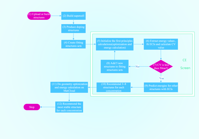
Figure 1: Schematic overview of the cluster expansion (CE) Screen process on MatCloud.

III.1 Clusters selection

We also employed the MIT ab initio Phase Stability(MAPS) cluster selection algorithm that was used in ATATVandeWalle2002 to facilitate cluster selection. It favors compact clusters and requires that all the sub-clusters of a many-body cluster are included in a CEZarkevich2004 ; Herder2015 . An input file containing parent lattice information is needed to use CE Screen. The clusters information are determined according to parent lattice data in the input file and its symmetry operations. The size of maximal cluster is determined by the radius cutoff specified by user, and we set the default value is the 8th nearest neighbor of parent structure referring to $N4R8$ criterionZhang2016 . For MatCloud platform, the input file will be automatically generated according to the initial structures uploaded by user. The formula has three parts, the first one is coordinate system containing lattice parameters data, the second is lattice vectors for the unit cell (either a primitive cell or a standard cell is ok), and the third are the atoms in the lattice, atoms include information of atomic symbols and atomic coordinates.

III.2 Fitting structures

In order to improve the calculation efficiency, we make some rules for structures in the fitting sets:

(1) The structures selected should cover all the concentrations, i.e., at least one structure has been selected per concentration;

(2) All the selected structures should be symmetrically in-equivalent structures.

and (3) The structures should include all different sized supercells if there is.

Structural relaxation and energy calculations are carried out for all structures in the fitting sets, calculation parameters in sectionII.3 are used. After all the first principles calculations are finished, the energies of these fitting structures will be extracted and their clusters identified by parent lattice are calculated at the same time. And then, the ECIs can be obtained through LSF by Eq.11. Using these ECIs, energies of other doping structures will be rapidly predicted using Eq.10. In order to assess the predictive power of the this tool, the cross validation(CV) score is used. It is defined as

$$CV=\left(\frac{1}{n}\sum_{i=1}^{n}(E_{i}-\hat{E}_{i})^{2}\right)^{\frac{1}{2}}$$ (12)

where $E_{i}$ is the calculated energy of structure $i$, while $\hat{E}_{i}$ is the predicted value of the energy of structure $i$ obtained from a LSF to the (n-1) other structural energies ($n$ is the fitting structure number). New calculated structures will be added to be used to fit ECIs until the CV is less than the tolerance users have set(The maximum CV value default is 50meV).

III.3 Applications on MatCloud

The CE Screen has been integrated into MatCloud, users just need to supply the initial structures which are used to be doped and the doping concentrations users are interested in, MatCloud will automatically call the CE Screen to recommend the stable structures for different concentrations. Users will receive an email when all the process are finished. Here is a brief outline of steps about CE Screen on MatCloud platform which is implemented in Fig.1.

(1)Upload (or build) initial structures in cif(crystallographic information file) or other formations.

Files containing parent lattice information will be generated.

(2)Construct supercells depending on your requirements. In this step, the input is a $3\times 3$ matrix.

(3)Produce doping structures.

(4)Create fitting structures sets.

When doped elements and concentrations are identified, MatCloud will produce all the required doping structures, and select structures by using symmetrically equivalent tool to create fitting structures sets. These structures are used to fit the ECIs.

(5)Initialize the first principles calculations.

MatCloud will automatically supply the calculated parameters according to the first principles code and tasks, users can change them if you would. MatCloud submit the jobs of geometry optimization and energy calculation for all fitting structures to HPC.

(6)$\sim$(8)Obtain the ECIs and its CV value.

All the energies of fitting structure are extracted after first principles calculations are finished, and then the ECIs will be fitted by using energy and cluster’s information of each calculated structure. Energies of all the fitting structures will be predicted with the ECIs, and the CV value is also computed. Add new structures to fitting structures sets and iterate steps (4)$\sim$(8) until maximum CE predictive reliability is obtained.

(9)and (10)Predict energies for all doping structures with the well fitted ECIs, and then recommend the stable structures with different concentrations for user.

After step (10), users can do first principles calculations for these recommended structures to select the lowest energy structure for each concentration.

Although there are many steps shown in Fig.1, time-consuming processes are handled by MatCloud. Users only need to wait for the e-mail notification of the job status after the information of (1)$\sim$(3) is identified. (4)$\sim$(10) is the process of CE Screen. It greatly improves the efficiency of selecting stable structures from multiple doping structures. In additions, MatCloud platform which integrates the supercell and doping structures construction, and EC Screen, make all the calculations more convenient.

IV Test cases

The CE Screen integrated in MatCloud can in principle be applied to any doping systems, i.e. substitution, vacancy, adsorption and interstitial sites. In this paper, we select the stable structures with different concentrations from all the doping structures for two systems, fcc Al-Ti and bcc Fe-Al. Al-Ti and Fe-Al are well-studied, technologically very important systemsChakraborty2010 ; Ghosh2008 . Hence, we choose these two systems as the prototypes to test our tools. In order to compare the calculated efficiency and make calculations executable, we select small amount structures. A fcc Al supercell of $2\times 1\times 1$ with dopant Ti is calculated, nine doping concentrations are considered: 0, $\frac{1}{8}$, $\frac{2}{8}$, $\cdots$ and 1. The number of all the doping structures is 257, and it is reduced to 27 after operating the crystallographic equivalence to all these initial doping structures. We calculated energies of all these 27 structures on MatCloud. We chose 20 doping structures randomly as fitting structures to predict energies for other 7 structures. The calculated and fitted formation energies for these 27 structures are shown in Fig.2. The formation energies for $Al_{1-x}Ti_{x}$ are calculated by

$$\Delta{E}=\frac{1}{8}E_{doped}-(1-x)E_{Al}-xE_{Ti}$$ (13)

Where, $E_{system}$ is the total energy for doped structure, $E_{Al}$ and $E_{Ti}$ are the atomic energy for per Al and Ti, respectively.

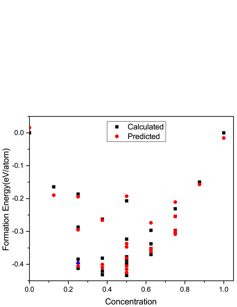
Figure 2: Formation energies for 27 $Al_{1-x}Ti_{x}$ structures from first principle calculations and CE Screen tools performed. Black squares denote energies from first principles, red circles denote energies predicted from CE Screen tools, and the blue upTriangles emphasize the predicted energies of structures which have been confirmed as the ground states from first principles.

We use all the 27 structures to fit a set of ECIs, and predict energies for these 27 structures. The CV value for $Al_{1-x}Ti_{x}$ is 0.021eV. The ground states for each concentration from first principles calculation and CE Screen tools are similar, except that the concentrations are 0.25. This error can be avoid by adding recommended structures number for each concentration.

Another example is a two-component Fe-Al system, a bcc Fe supercell of $2\times 2\times 2$ with dopant Al. To study the solution doping effects on Fe supercell, seventeen doping concentrations are considered: 0, $\frac{1}{16}$, $\frac{2}{16}$, $\cdots$, and 1. The number of all the doping structures is 65536, and it is reduced to 331 after operating the crystallographic equivalence to all these initial doping structures. To select the stable structures for each concentration, usually we need to calculate all the structures with different concentrations. CE Screen tools will speed up this process, it only needs at most to calculate 100 structures according to our rules. We firstly chose 30 doping structures following the rules depicted in sectionIII.2 as fitting structures sets. The calculated CV value for $Fe_{1-x}Al_{x}$ is 0.04eV, satisfying the default tolerance (50meV). And then use the fitted ECIs and the cluster’s information of the rest 301 structures to predict their energies. The second step is first principles calculations for selected 8 structures from each concentration, and we should make sure that the number of all structures needed to be calculated is less than 100. The calculated and predicted formation energies for these 331 structures are shown in Fig.3. The formation energies for $Fe_{1-x}Al_{x}$ are calculated by

$$\Delta{E}=\frac{1}{16}E_{doped}-(1-x)E_{Al}-xE_{Ti}$$ (14)

Where, $E_{doped}$ is the total energy for doped structure, $E_{Fe}$ and $E_{Al}$ are the atomic energy for per Fe and Al, respectively.

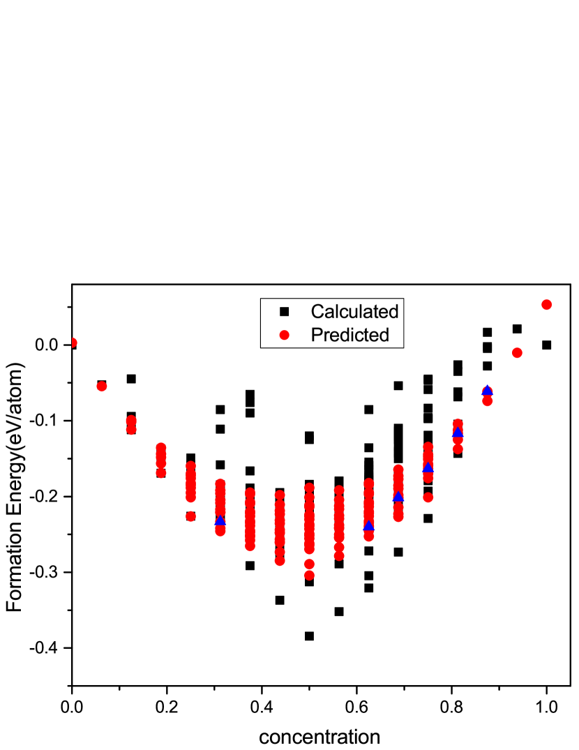
Figure 3: Formation energies for 331 $Fe_{1-x}Al_{x}$ structures from first principle calculations and CE Screen tools performed. Black squares denote energies from first principles, red circles denote energies predicted from CE Screen tools, and the blue upTriangles emphasize the predicted energies of structures which have been confirmed as the ground states from first principles.

From Fig.3, although not all the most stable structure are predicted exactly, the ground states for each concentration are all sit in the candidates. The largest number of structures to be calculated is 5 when concentration is $\frac{12}{16}$. It’s worth mentioning that the most stable structures predicted from CE Screen tool are the same as that calculated from first principles calculations when the concentrations are 0, $\frac{1}{16}$, $\frac{2}{16}$ , $\frac{3}{16}$, $\frac{4}{16}$, $\frac{6}{16}$, $\frac{7}{16}$, $\frac{8}{16}$, $\frac{9}{16}$, $\frac{15}{16}$, and $1$. From the calculated results, we can claim that the ground states for other concentrations can be well predicted by calculating at most 5 additional doping structures.

V Conclusions

To truly predict the structure of a doping compound, we firstly must find the lowest-energy structure at a concentration. In this paper, we developed a method to select stable structures for different doping concentrations with a small number of first principles calculations. This method has combined approach of first-principles calculations and cluster expansion method, and it beautifully solves the problem that quickly selecting lowest-energy structures from a huge number of known structures. This method has been packaged into a tool, named as CE Screen, and it will be download from address of MatCloud (http://matcloud.cnic.cn) soon. The tool has been integrated into MatCloud platform which developed by our group, and this makes it simple and easy for all the users.

In application cases, energy calculations of two doping systems have been carried out employing two different methods. One is completely first principles calculations, the other is using CE Screen. By using CE Screen on Matcloud, the survey of only 30 symmetrically in-equivalent configurations is sufficient to find the ground state structure of $Fe_{1-x}Al_{x}$ within the whole range of the concentrations. Although a worse result for hcp structures has been published, a better-converged result can be achieved by increasing relatively more input fitting structures.

Although CE Screen developed by our group is only suitable for structures derived from a parent lattice, it will be a powerful tool for evaluating the stability of these structures. Two important facts should be pointed if you want to use this tool on MatCloud. One is that the number of input fitting structures required for the CE Screen is started from 30, it also varies from system to system. The other is that first principle codes of Abinit, VASP, CASTEP, PWSCF, $\cdots$, are all supported by CE Screen and MatCloud, however, users should supply the license if you want to use commercial softwares such as VASP and CASTEP.

References

- [1] Wahyu Setyawan and Stefano Curtarolo. High-throughput electronic band structure calculations: Challenges and tools. Computational Materials Science, 49(2):299–312, aug 2010.
- [2] Cyrus Kalil Tom And Wadia. Materials Genome Initiative for Global Competitiveness. Genome, (June):1–18, 2011.
- [3] Stefano Curtarolo, Wahyu Setyawan, Gus L.W. Hart, Michal Jahnatek, Roman V. Chepulskii, Richard H. Taylor, Shidong Wang, Junkai Xue, Kesong Yang, Ohad Levy, Michael J. Mehl, Harold T. Stokes, Denis O. Demchenko, and Dane Morgan. AFLOW: An automatic framework for high-throughput materials discovery. Computational Materials Science, 58:218–226, jun 2012.
- [4] Anubhav Jain, Shyue Ping Ong, Geoffroy Hautier, Wei Chen, William Davidson Richards, Stephen Dacek, Shreyas Cholia, Dan Gunter, David Skinner, Gerbrand Ceder, and Kristin a. Persson. Commentary: The materials project: A materials genome approach to accelerating materials innovation. APL Materials, 1:001002, 2013.
- [5] Qu Wu, Bing He, Tao Song, Jian Gao, and Siqi Shi. Cluster expansion method and its application in computational materials science. Computational Materials Science, 125:243–254, 2016.
- [6] Monodeep Chakraborty, Jürgen Spitaler, Peter Puschnig, and Claudia Ambrosch-Draxl. ATAT@WIEN2k: An interface for cluster expansion based on the linearized augmented planewave method. Computer Physics Communications, 181(5):913–920, 2010.
- [7] A. van de Walle and G Ceder. Automating first-principles phase diagram calculations. Journal of Phase Equilibria, 23(4):348–359, 2002.
- [8] C Ravi, H K Sahu, M C Valsakumar, and Axel van de Walle. Cluster expansion Monte Carlo study of phase stability of vanadium nitrides. Physical Review B, 81(10):104111, 2010.
- [9] Evgeni S Penev, Somnath Bhowmick, Arta Sadrzadeh, and Boris I Yakobson. Polymorphism of Two-Dimensional Boron. (1):2441–2445, 2012.
- [10] Xi Bo Li, Pan Guo, D. Wang, Yongsheng Zhang, and Li Min Liu. Adaptive cluster expansion approach for predicting the structure evolution of graphene oxide. Journal of Chemical Physics, 141(22), 2014.
- [11] Alex Kutana, Evgeni S Penev, and Boris I Yakobson. Engineering electronic properties of layered transition-metal dichalcogenide compounds through alloying. Nanoscale, 6(11):5820–5825, 2014.
- [12] J. M. Sanchez, F. Ducastelle, and D. Gratias. Generalized cluster description of multicomponent systems. Physica A: Statistical Mechanics and its Applications, 128(1-2):334–350, 1984.
- [13] C. Wolverton, G. Ceder, D. De Fontaine, and H. Dreyssé. Ab initio determination of structural stability in fcc-based transition-metal alloys. Physical Review B, 48(2):726–747, 1993.
- [14] C. Wolverton and D. De Fontaine. Cluster expansions of alloy energetics in ternary intermetallics. Physical Review B, 49(13):8627–8642, 1994.
- [15] Alex Zunger, L G Wang, Gus L W Hart, and Mahdi Sanati. Obtaining Ising-like expansions for binary alloys from first principles. Modelling and Simulation in Materials Science and Engineering, 10(6):685–706, 2002.
- [16] Laura M. Herder, Jason M. Bray, and William F. Schneider. Comparison of cluster expansion fitting algorithms for interactions at surfaces. Surface Science, 640:104–111, 2015.
- [17] Nikolai A. Zarkevich and D. D. Johnson. Reliable first-principles alloy thermodynamics via truncated cluster expansions. Physical Review Letters, 92(25 I):255702–1, 2004.
- [18] Xi Zhang and Marcel H F Sluiter. Cluster Expansions for Thermodynamics and Kinetics of Multicomponent Alloys. Journal of Phase Equilibria and Diffusion, 37(1):44–52, 2016.
- [19] G. Ghosh, A. van de Walle, and M. Asta. First-principles calculations of the structural and thermodynamic properties of bcc, fcc and hcp solid solutions in the Al-TM (TM = Ti, Zr and Hf) systems: A comparison of cluster expansion and supercell methods. Acta Materialia, 56(13):3202–3221, 2008.