Properties of 2+1-flavor QCD in the imaginary chemical potential region: model approach

Abstract

We study properties of 2+1-flavor QCD in the imaginary chemical potential region by using two approaches. One is a theoretical approach based on QCD partition function, and the other is a qualitative one based on the Polyakov-loop extended Nambu–Jona-Lasinio (PNJL) model. In the theoretical approach, we clarify conditions imposed on the imaginary chemical potentials $\mu_{f}=i\theta_{f}T$ to realize the Roberge-Weiss (RW) periodicity. Here, $T$ is temperature, the index $f$ denotes the flavor, and $\theta_{f}$ are dimensionless chemical potentials. We also show that the RW periodicity is broken if anyone of $\theta_{f}$ is fixed to a constant value. In order to visualize the condition, we use the PNJL model as a model possessing the RW periodicity, and draw the phase diagram as a function of $\theta_{u}=\theta_{d}\equiv\theta_{l}$ for two conditions of $\theta_{s}=\theta_{l}$ and $\theta_{s}=0$. We also consider two cases, $(\mu_{u},\mu_{d},\mu_{s})=(i\theta_{u}T,iC_{1}T,0)$ and $(\mu_{u},\mu_{d},\mu_{s})=(iC_{2}T,iC_{2}T,i\theta_{s}T)$; here $C_{1}$ and $C_{2}$ are dimensionless constants, whereas $\theta_{u}$ and $\theta_{s}$ are treated as variables. For some choice of $C_{1}$ ($C_{2}$), the number density of up (strange) quark becomes smooth in the entire region of $\theta_{u}$ ($\theta_{s}$) even in high $T$ region. This property may be important for lattice QCD simulations in the imaginary chemical potential region, since it makes the analytic continuation more feasible.

I INTRODUCTION

One of the most important issues in hadron physics is to clarify properties of quark matter in finite temperature and/or quark chemical potential. The knowledge of thermodynamics on quark matter is essential to understand structure of the QCD phase diagram. As the review of the QCD phase diagram, see Refs. Stephanov ; Munzinger-Wambach ; Fukushima-Hatsuda ; Fukushima-Sasaki and references therein.

Lattice QCD (LQCD) simulations may be the most promising and powerful theoretical tool of investigating the QCD phase diagram. As for isospin-symmetric 2-flavor QCD, the fermion matrix is written as

$$\mathcal{M}(\mu_{l})=\gamma_{\mu}D_{\mu}+m_{l}-\gamma_{4}\mu_{l},$$ (1)

and satisfies $\gamma_{5}$-hermiticity, $(\mathcal{M}(\mu_{l}))^{{\dagger}}=\gamma_{5}\mathcal{M}(-\mu_{l})\gamma_{5}$. Here, $\mu_{l}$ and $m_{l}$ are the light-quark chemical potential and its mass, respectively. LQCD simulations are feasible for $\mu_{l}=0$ since $\textrm{det}\mathcal{M}(0)$ is real and positive definite. However, the fermion determinant becomes complex in finite $\mu_{l}$ because $\left(\textrm{det}\mathcal{M}(\mu_{l})\right)^{\ast}=\textrm{det}\mathcal{M}(-\mu_{l})\neq\textrm{det}\mathcal{M}(\mu_{l})$ from the $\gamma_{5}$-hermiticity. This is the well-known sign problem and makes the importance-sampling method unfeasible.

One of ideas to circumvent the sign problem is the imaginary chemical potential $\mu_{l}=i\theta_{l}T$, where $T$ is temperature and $\theta_{l}$ is a dimensionless chemical potential. Indeed, the relation

$$(\mathcal{M}(i\theta_{l}T))^{{\dagger}}=\gamma_{5}\mathcal{M}(i\theta_{l}T)\gamma_{5}$$ (2)

can be obtained and hence there is no sign problem, and positivity of the fermion determinant is also ensured. From the imaginary $\mu_{l}$ region, one can extract information of the real $\mu_{l}$ region by the analytic continuation. In fact, this approach was successful for the 2-flavor QCD Forcrand-Philipsen1 ; DElia-Lombard ; Wu-Luo-Chen ; DElia-Sanfilippo ; Forcrand-Philipsen2 ; Nagata-Nakamura ; Cea_two_flavor ; Takahashi1 ; Bonati_chiral_transition ; Takahashi2 .

In the imaginary $\mu_{l}$ region, the QCD thermodynamic potential has the Roberge-Weiss (RW) periodicity bib_Roberge-Weiss , which can be regarded as a remnant of $\mathbb{Z}_{3}$ symmetry in the pure gauge limit. Also in Ref. bib_Roberge-Weiss , it was shown that the first-order RW phase transition occurs at $\theta_{l}=(2k+1)\pi/3$ above some temperature $T_{\rm RW}$, where $k$ is any integer; see Fig. 1. Due to the RW phase transition, information of the real $\mu_{l}$ region is limited up to $\mu_{l}/T\sim 1$, particularly at $T>T_{\rm RW}$.

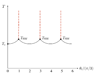
Fig. 1: Sketch of the QCD phase diagram in $\theta_{l}$-$T$ plane. The solid line is the crossover deconfinement transition line and the vertical dashed line is the first-order RW phase transition line. The deconfinement transition temperature is represented by $T_{\rm c}$. The label $T_{\rm RW}$ means the RW phase transition temperature.

As an alternative method of LQCD simulations, one can consider effective models. Among effective models, the Polyakov-loop extended Nambu–Jona-Lasinio (PNJL) model is one of the most useful models and yields good description of phenomena on quark matter, such as chiral and deconfinement transitions Meisinger ; Dumitru ; Fukushima1 ; Ghos ; Megias ; Ratti1 ; Rossner ; Kashiwa_PNJL ; Sakai_PRD77_051901 ; Sakai_PRD78_036001 ; Sakai_PRD78_076007 ; Sakai_PRD79_096001 ; Sakai_JPhys . It was proven in Refs. Sakai_PRD77_051901 ; Sakai_PRD78_036001 ; Sakai_PRD78_076007 ; Sakai_PRD79_096001 that the thermodynamic potential of the PNJL model possesses the RW periodicity for the 2-flavor case, and the PNJL model reasonably reproduces LQCD data on the imaginary $\mu_{l}$ region Sakai_PRD79_096001 ; Sakai_JPhys .

In the case of 2+1-flavor QCD, the strange-quark chemical potential $\mu_{s}$ is introduced as an additional external parameter, and the fermion determinant consists of the product $\textrm{det}\mathcal{M}(\mu_{l})\cdot\textrm{det}\mathcal{M}(\mu_{s})$. When both $\mu_{l}$ and $\mu_{s}$ are pure imaginary, that is, when $\mu_{l}=i\theta_{l}T$ and $\mu_{s}=i\theta_{s}T$, the fermion determinant becomes real and positivity of its determinant is guaranteed just as in the 2-flavor case. Here, $\theta_{s}$ is a dimensionless chemical potential for strange quark. It is thus suitable to consider the imaginary chemical potential region even in the 2+1-flavor case, and some works were carried out Cea ; Bonati ; Bonati2 ; Bonati3 ; DElia-Gagliardi-Sanfilippo . In Ref Bonati , the one-loop effective potential for the untraced Polyakov loop in the high $T$ limit was calculated as a function of $\theta_{l}$ for two conditions, (I) $\theta_{s}=\theta_{l}$ and (II) $\theta_{s}=0$, and they showed that the RW periodicity exists only in condition (I). In addition to this result, the calculation in non-perturbative region is also necessary to acquire better understanding of the RW phase transition.

Also in Ref. Bonati , it was pointed out that the $\theta_{l}$ region available for analytic continuation becomes broader in condition (II) than (I). This fact indicates that the analytic region can be expanded by breaking the RW periodicity deliberately. It is, therefore, interesting to consider how largely the analytic region is expanded by breaking the RW periodicity.

In this paper, we study properties of the 2+1-flavor QCD in the imaginary chemical potential region by using two approaches. One is a theoretical approach based on the QCD partition function, and the other is a qualitative one based on the PNJL model. In the theoretical approach, we first prove that the thermodynamic potential of non-degenerate three-flavor QCD has the RW periodicity in general, but the periodicity is lost when anyone of the chemical potentials is fixed to a constant value. Next, as for the 2+1-flavor case, we prove that the thermodynamic potential of the PNJL model has the same properties of QCD on the RW periodicity. For this reason, the PNJL model is used for qualitative analysis. We calculate some thermodynamic quantities and draw the phase diagram by using the PNJL model under conditions (I) and (II) in order to visualize roles of the conditions. Finally, we evaluate up- and strange-quark number densities for some choices of $\theta_{l}$ and $\theta_{s}$. We numerically confirm that discontinuity of number densities due to the first-order phase transition disappears in high $T$ region, and the number densities become smooth. This property may be important for LQCD simulations in the imaginary chemical potential region, since it makes the analytic continuation more feasible even in high $T$ region.

This paper is organized as follows: In Sec. II, we discuss the relation between the QCD thermodynamic potential and the RW periodicity. In Sec. III, formalism of the PNJL model is explained, and the properties of the model in the imaginary chemical potential region is discussed. Sec. IV is devoted to present numerical results calculated by the PNJL model. The summary is given in Sec. V.

II QCD PARTITION FUNCTION AND RW PERIODICITY

Before going to the 2+1-flavor case, we consider non-degenerate three-flavor QCD with imaginary $\mu_{f}$ $(f=u,d,s)$. For later convenience, we introduce the dimensionless chemical potentials $\theta_{f}$ as $\mu_{f}=i\theta_{f}T$. In Euclidean spacetime with the time interval $\tau\in[0,\beta=1/T]$, the QCD partition function $Z_{\rm QCD}$ is defined by

$$Z_{\rm QCD}(\theta_{f})=\int\mathcal{D}A\mathcal{D}\bar{q}\mathcal{D}q\exp\left[-S_{\rm QCD}\right]$$ (3)

having the action

$$S_{\rm QCD}=\int d^{4}x\left[\bar{q}\left(\gamma_{\mu}D_{\mu}+\hat{m}-i\frac{\hat{\theta}}{\beta}\gamma_{4}\right)q+\frac{1}{4g^{2}}\left(F^{a}_{\mu\nu}\right)^{2}\right],$$ (4)

where $q=(q_{u},q_{d},q_{s})^{\rm T}$ is the quark field, $\hat{m}=\textrm{diag}(m_{u},m_{d},m_{s})$ is the current-quark mass matrix, and $D_{\mu}=\partial_{\mu}+iA_{\mu}$ is the covariant derivative including the gluon field $A_{\mu}=gA^{a}_{\mu}\lambda^{a}/2$ with the gauge coupling $g$ and the Gell-Mann matrices $\lambda^{a}$. For the quark fields, the anti-periodic boundary conditions $q_{f}(\beta,\mathbf{x})=-q_{f}(0,\mathbf{x})$ are imposed. The dimensionless chemical-potential matrix $\hat{\theta}$ is defined by $\hat{\theta}=\textrm{diag}(\theta_{u},\theta_{d},\theta_{s})$.

We first redefine all the quark fields as

$$q_{f}\rightarrow\exp\left[i\frac{\theta_{f}}{\beta}\tau\right]q_{f}.$$ (5)

The integral measure is unchanged under Eq. (5) and $Z_{\rm QCD}$ is transformed into

$$\begin{aligned} &Z_{\rm QCD}(\theta_{f})=\int\mathcal{D}A\mathcal{D}\bar{q}\mathcal{D}q\exp\left[-S_{\rm QCD}\right],\\ &S_{\rm QCD}=\int d^{4}x\left[\bar{q}(\gamma_{\mu}D_{\mu}+\hat{m})q+\frac{1}{4g^{2}}\left(F^{a}_{\mu\nu}\right)^{2}\right]\end{aligned}$$ (6)

with the boundary conditions

$$q_{f}(\beta,\mathbf{x})=-\textrm{e}^{i\theta_{f}}q_{f}(0,\mathbf{x}).$$ (7)

Now, we consider $\mathbb{Z}_{3}$ transformation defined by

$$q_{f}\rightarrow U_{k}q_{f},$$ (8)

$$A_{\mu}\rightarrow U_{k}A_{\mu}U^{-1}_{k}+i(\partial_{\mu}U_{k})U^{-1}_{k},$$ (9)

$$U_{k}=\exp\left[i\frac{2\pi k}{3}\frac{\tau}{\beta}\right],\ \ k\in\mathbb{Z}.$$ (10)

The functional form of $Z_{\rm QCD}$ keeps the form of Eq. (6) under the $\mathbb{Z}_{3}$ transformation, but the boundary conditions are changed into

$$q_{f}(\beta,\mathbf{x})=-\exp\left[i\left(\theta_{f}-\frac{2\pi k}{3}\right)\right]q_{f}(0,\mathbf{x}).$$ (11)

Equations (6), (7) and (11) give the equality

$$Z_{\rm QCD}(\theta_{f}-2\pi k/3)=Z_{\rm QCD}(\theta_{f}).$$ (12)

The QCD partition function thus has the periodicity of $2\pi/3$ in $\theta_{f}$, which is nothing but the RW periodicity.

The RW periodicity of $Z_{\rm QCD}$ can be interpreted as the invariance under the extended $\mathbb{Z}_{3}$ transformation Sakai_PRD77_051901 ; Sakai_PRD78_036001 ; Sakai_PRD78_076007 ; Sakai_PRD79_096001 , composed of the shift $\theta_{f}\ \rightarrow\theta_{f}+2\pi k/3$ and Eqs. (8) - (10). The QCD thermodynamic potential $\Omega_{\rm QCD}$ (per unit volume) is related with $Z_{\rm QCD}$ as $\Omega_{\rm QCD}=-T\ln Z_{\rm QCD}$. Therefore, $\Omega_{\rm QCD}$ also has the RW periodicity when $Z_{\rm QCD}$ is invariant under the extended $\mathbb{Z}_{3}$ transformation.

The discussions mentioned above can be applied to the 2+1-flavor case by setting $\theta_{u}=\theta_{d}\equiv\theta_{l}$. Hence, one can find that $\Omega_{\rm QCD}$ with condition (I) has the RW periodicity because of its invariance under the extended $\mathbb{Z}_{3}$ transformation. Meanwhile, when any one of $\theta_{f}$ is fixed to a constant value, for example $\theta_{s}=0$ in condition (II), the RW periodicity disappears anymore since one cannot make the shift $\theta_{f}\rightarrow\theta_{f}+2\pi k/3$ for fixed $\theta_{f}$. This is the reason why the RW periodicity does not exist for condition (II). In the next section, we formulate the 2+1-flavor PNJL model and show that the PNJL model also possesses the same properties discussed in this section.

III PNJL MODEL

The Lagrangian of PNJL model in Euclidean spacetime is formulated by

$$\mathcal{L}_{\rm PNJL}= \bar{q}\left(\gamma_{\mu}D_{\mu}+\hat{m}-i\frac{\hat{\theta}}{\beta}\gamma_{4}\right)q+\mathcal{U}$$

$$-G_{\rm s}\sum_{a=0}^{8}\left[(\bar{q}\lambda^{a}q)^{2}+(\bar{q}i\gamma^{5}\lambda^{a}q)^{2}\right]$$

$$+K\left[\textrm{det}_{f}\bar{q}(1+\gamma^{5})q+\textrm{det}_{f}\bar{q}(1-\gamma^{5})q\right],$$ (13)

where the definitions of $q$, $\hat{m}$ and $\hat{\theta}$ are the same as in Eq. (4), but the covariant derivative has the form $D_{\mu}=\partial_{\mu}+ig\delta_{\mu 4}A^{a}_{\mu}\lambda^{a}/2$ in the present PNJL model. The Polyakov-loop potential $\mathcal{U}$ is a function of Polyakov loop $\Phi$ and its conjugate $\Phi^{\ast}$. The definitions of these quantities are

$$\Phi=\frac{1}{3}{\rm Tr}_{\rm c}(L),\ \ \ \Phi^{\ast}=\frac{1}{3}{\rm Tr}_{\rm c}({L}^{{\dagger}}),$$ (14)

where $L=\exp[i\beta A_{4}]=\exp[i\beta{\rm diag}(A_{4}^{11},A_{4}^{22},A_{4}^{33})]$ for the classical gauge fields $A_{4}^{ii}$ satisfying $A_{4}^{11}+A_{4}^{22}+A_{4}^{33}=0$, and the trace is taken in color space. We use the logarithm type of

$$\mathcal{U}=T^{4}\left[-\frac{a(T)}{2}\Phi\Phi^{\ast}+b(T)\ln H\right],$$ (15)

$$a(T)=a_{0}+a_{1}\left(\frac{T_{0}}{T}\right)+a_{2}\left(\frac{T_{0}}{T}\right)^{2},\ b(T)=b_{3}\left(\frac{T_{0}}{T}\right)^{3},$$ (16)

$$H=1-6\Phi\Phi^{\ast}+4(\Phi^{3}+\Phi^{\ast 3})-3(\Phi\Phi^{\ast})^{2}$$ (17)

in Ref. Rossner . Note that Eq. (15) preserves the $\mathbb{Z}_{3}$ symmetry.

The original value of $T_{0}$ is fitted to 270 MeV so as to reproduce the deconfinement transition temperature in the pure gauge limit Boyd ; Kaczmarek . When the dynamical quarks are taken into account, the value of $T_{0}=270$ MeV predicts higher deconfinement transition temperature than LQCD prediction, $T_{\rm c}\sim 160$ MeV at $\theta_{f}=0$ Fodor_Katz_tem ; Borsanyi ; Soldner ; Kanaya ; Laermann . The calculation in Ref. Sasaki_EPNJL provides lower $T_{\rm c}$ at $\theta_{f}=0$ by refitting $T_{0}$ to a lower value, but we keep the original value to concentrate on qualitative discussions.

In the quark-quark interaction terms, $G_{\rm s}$ is the strength of the scalar-type four-point interaction and $K$ is the strength of the Kobayashi-Maskawa-’t Hooft (KMT) interaction tHooft ; Kobayashi-Maskawa ; Kobayashi-Kondo-Maskawa . The determinant in the KMT interaction term is taken in flavor space. The KMT interaction explicitly breaks $\textrm{U}_{\rm A}(1)$ symmetry and is necessary to reproduce the measured mass of $\eta^{\prime}$ meson at vacuum.

The mean-field approximation yields the thermodynamic potential $\Omega_{\rm PNJL}$ (per unit volume) as

$$\Omega_{\rm PNJL}=2G_{\rm s}\sum_{f=u,d,s}\sigma^{2}_{f}-4K\sigma_{u}\sigma_{d}\sigma_{s}+\mathcal{U}$$

$$-\frac{2}{\beta}\sum_{f=u,d,s}\int\frac{d^{3}\mathbf{p}}{(2\pi)^{3}}\bigl{[}3\beta E_{f}$$

$$+\ln(1+3\Phi\textrm{e}^{-\beta(E_{f}-\mu_{f})}+3\Phi^{\ast}\textrm{e}^{-2\beta(E_{f}-\mu_{f})}+\textrm{e}^{-3\beta(E_{f}-\mu_{f})})$$

$$+\ln(1+3\Phi^{\ast}\textrm{e}^{-\beta(E_{f}+\mu_{f})}+3\Phi\textrm{e}^{-2\beta(E_{f}+\mu_{f})}+\textrm{e}^{-3\beta(E_{f}+\mu_{f})})\bigr{]},$$ (18)

where $\mu_{f}=i\theta_{f}T$, $\sigma_{f}=\braket{\bar{q}_{f}q_{f}}$ and $E_{f}=\sqrt{\mathbf{p}^{2}+M^{2}_{f}}$ with the constituent-quark masses

$$\begin{aligned} &M_{f}=m_{f}-4G_{\rm s}\sigma_{f}+2K\sigma_{f^{\prime}}\sigma_{f^{\prime\prime}},\\ &\left(f\neq f^{\prime},\ \ f^{\prime}\neq f^{\prime\prime},\ \ f\neq f^{\prime\prime}\right).\end{aligned}$$ (19)

Note that $\theta_{u}=\theta_{d}\equiv\theta_{l}$, $\sigma_{u}=\sigma_{d}$ and $E_{u}=E_{d}$ in the 2+1-flavor case. We introduce the three-dimensional cutoff $\Lambda$ to regularize the vacuum term in Eq. (18). The variables $X=\left\{\sigma_{l},\sigma_{s},\Phi,\Phi^{\ast}\right\}$ are determined by the stationary conditions,

$$\frac{\partial\Omega_{\rm PNJL}}{\partial X}=0,\ \ X=\left\{\sigma_{l},\sigma_{s},\Phi,\Phi^{\ast}\right\}.$$ (20)

The parameters used in the present PNJL model are summarized in TABLE 1.

Table 1: Summary of the parameter set used in the present PNJL model. The panels (a) and (b) are the parameter set in $\mathcal{U}$ Rossner and the NJL part  Reinberg_Klevansky_Hufner ; Klevansky_review , respectively.

(a)	$a_{0}$	$a_{1}$	$a_{2}$	$b_{3}$	$T_{0}$ [MeV]
	3.51	- 2.47	15.2	- 1.75	270
(b)	$m_{l}$ [MeV]	$m_{s}$ [MeV]	$\Lambda$ [MeV]	$G_{\rm s}\Lambda^{2}$	$K\Lambda^{5}$
	5.5	140.7	602.3	1.835	12.36

Under the extended $\mathbb{Z}_{3}$ transformation, the Polyakov loop behaves as $\Phi\rightarrow\Phi\textrm{e}^{-2\pi ik/3}$ and is not invariant. It is more convenient to define the flavor-dependent modified Polyakov loop and its conjugate Sakai_JPhys as

$$\Psi_{f}=\textrm{e}^{i\theta_{f}}\Phi,\ \ \Psi^{\ast}_{f}=\textrm{e}^{-i\theta_{f}}\Phi^{\ast}.$$ (21)

The extended $\mathbb{Z}_{3}$ transformation leaves these quantities invariant. After rewriting Eq. (18) by $\Psi_{f}$ and $\Psi^{\ast}_{f}$, we can reach the expression

$$\Omega_{\rm PNJL}=2G_{\rm s}\sum_{f=u,d,s}\sigma^{2}_{f}-4K\sigma_{u}\sigma_{d}\sigma_{s}+\mathcal{U}$$

$$-\frac{2}{\beta}\sum_{f=u,d,s}\int\frac{d^{3}\mathbf{p}}{(2\pi)^{3}}\bigl{[}3\beta E_{f}$$

$$+\ln(1+3\Psi_{f}\textrm{e}^{-\beta E_{f}}+3\Psi^{\ast}_{f}\textrm{e}^{-2\beta E_{f}}\textrm{e}^{3i\theta_{f}}+\textrm{e}^{-3\beta E_{f}}\textrm{e}^{3i\theta_{f}})$$

$$+\ln(1+3\Psi^{\ast}_{f}\textrm{e}^{-\beta E_{f}}+3\Psi_{f}\textrm{e}^{-2\beta E_{f}}\textrm{e}^{-3i\theta_{f}}+\textrm{e}^{-3\beta E_{f}}\textrm{e}^{-3i\theta_{f}})\bigr{]}.$$ (22)

The $\theta_{f}$-dependence of Eq. (22) is embedded in the extended $\mathbb{Z}_{3}$ symmetric quantities $\{\textrm{e}^{\pm 3i\theta_{f}},\Psi_{f},\Psi^{\ast}_{f}\}$. Obviously, $\Omega_{\rm PNJL}$ is invariant under the extended $\mathbb{Z}_{3}$ transformation and hence $\Omega_{\rm PNJL}$ has the RW periodicity in general. Once any one of $\theta_{f}$ is fixed to some constant value, however, the extended $\mathbb{Z}_{3}$ transformation changes $\Psi_{f}$ into $\Psi_{f}\textrm{e}^{-2\pi ik/3}$ and thereby $\Omega_{\rm PNJL}$ does not become invariant. It is thus concluded that $\Omega_{\rm PNJL}$ has the same properties as $\Omega_{\rm QCD}$ on the RW periodicity.

IV NUMERICAL RESULTS

We show numerical results calculated by the PNJL model. In calculations of thermodynamic quantities and the QCD phase diagram, both conditions (I) and (II) are considered. We pick up $\Omega_{\rm PNJL}$ and the quark number density $n_{q}$ as the thermodynamic quantities, and calculate $\theta_{l}$-dependence for $T=200,250$ MeV. In the results of condition (I), the RW periodicity can be seen. On the contrary, there is no RW periodicity for condition (II), as expected in Sec. III. In the QCD phase diagram, we find for condition (II) that the crossover chiral transition line is discontinuous at some value of $\theta_{l}$. In addition, the first-order phase transition line appears as is the RW phase transition line, and can be fitted by a polynomial function of $\theta_{l}$. Finally, the up- and strange-quark number densities are calculated under the situation that no RW periodicity exists. We show that the non-analyticity in the number densities disappears below some constant value of $\theta_{l}$ or $\theta_{s}$.

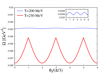
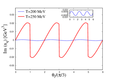
Fig. 2: The $\theta_{l}$-dependence of $\Omega_{\rm PNJL}$ and the imaginary part of the quark number density $\textrm{Im}(n_{q})$ calculated by the PNJL model for condition (I). The solid line is the results for $T=250$ MeV and the dotted line for $T=200$ MeV.

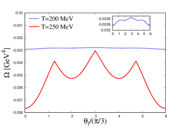
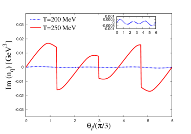
Fig. 3: The $\theta_{l}$-dependence of $\Omega_{\rm PNJL}$ and the imaginary part of the quark number density $\textrm{Im}(n_{q})$ calculated by the PNJL model for condition (II). The meanings of each line are same as in Fig. 2.

IV.1 BEHAVIOR OF THERMODYNAMIC QUANTITIES

The quark number density $n_{q}$ is obtained by the relation

$$n_{q}=\sum_{f=u,d,s}n_{f}=i\beta\sum_{f=u,d,s}\frac{\partial}{\partial\theta_{f}}\Omega_{\rm PNJL},$$ (23)

where $n_{f}$ is the number density of the quark with flavor $f$. Using Eq. (23), we can see that the condition to exist the RW periodicity in $n_{q}$ is equivalent to that in $\Omega_{\rm PNJL}$. Since $\Omega_{\rm PNJL}$ is charge-even, $n_{f}$ is charge-odd; Namely, $\Omega_{\rm PNJL}(\theta_{f})=\Omega_{\rm PNJL}(-\theta_{f})$ and $n_{q}(-\theta_{f})=-n_{q}(\theta_{f})$.

Figure 2 presents $\Omega_{\rm PNJL}$ and the imaginary part of $n_{q}$, $\textrm{Im}(n_{q})$, for condition (I), as a function of $\theta_{l}$. The dotted line denotes the results for $T=200$ MeV and the solid line does for $T=250$ MeV. Both $\Omega_{\rm PNJL}$ and $n_{q}$ have the RW periodicity and are smooth for any $\theta_{l}$ when $T=200$ MeV. Meanwhile, $\Omega_{\rm PNJL}$ has cusps at $\theta_{l}=\pi/3$ mod $2\pi/3$ and $n_{q}$ becomes discontinuous there for $T=250$ MeV. These singularities mean the first-order RW phase transition, and indicate that the RW endpoint is located in $200<T<250$ MeV (see Fig 4).

Now, we concentrate on the region of $0\leq\theta_{l}\leq 2\pi/3$. For charge-even quantities $\mathcal{O}_{\rm even}$ with the RW periodicity, such as $\Omega_{\rm PNJL}$, the relation

$$\mathcal{O}_{\rm even}(\theta_{l}-\epsilon) =\mathcal{O}_{\rm even}(-\theta_{l}+\epsilon)$$

$$=\mathcal{O}_{\rm even}(-\theta_{l}+2\pi/3+\epsilon)$$ (24)

is obtained, where $\epsilon$ is a positive infinitesimal quantity. If the gradient

$$\lim_{\theta_{l}\rightarrow\pi/3\pm 0}\frac{d\mathcal{O}_{\rm even}}{d\theta_{l}}$$ (25)

is neither zero nor infinity, charge-even quantities have a cusp at $\pi/3$. On the other hand, charge-odd quantities $\mathcal{O}_{\rm odd}$ possessing the RW periodicity, such as $\textrm{Im}(n_{q})$, satisfy

$$\mathcal{O}_{\rm odd}(\theta_{l}-\epsilon) =-\mathcal{O}_{\rm odd}(-\theta_{l}+\epsilon)$$

$$=-\mathcal{O}_{\rm odd}(-\theta_{l}+2\pi/3+\epsilon).$$ (26)

Hence, discontinuity is seen at $\theta_{l}=\pi/3$ for charge-odd quantities in high $T$ region Sakai_PRD77_051901 ; Sakai_PRD78_036001 ; Sakai_PRD78_076007 ; Kouno_JPhys , where

$$\lim_{\theta_{l}\rightarrow\pi/3\pm 0}\mathcal{O}_{\rm odd}(\theta_{l})\neq 0.$$ (27)

Due to these singularities, the analytic continuation from the imaginary $\mu_{l}$ to the real one is limited up to $\theta_{l}=\pi/3$, particularly for the high $T$ region.

Figure 3 is same as Fig. 2, but for condition (II). It is clearly seen that the RW periodicity is lost, but $\theta_{l}$-dependence is similar to each other between Figs. 2 and 3. In particular, the first-order phase transition still takes place for $T=250$ MeV, and it is expected that its endpoint is located in $200<T<250$ MeV (see Fig. 5). We refer to this transition as the first-order “RW-like phase transition”. It should be noted that the RW-like phase transition occurs at $\theta_{l}=0.42\pi$ for $T=250$ MeV. This result indicates that the region needed to the analytic continuation becomes broader for condition (II) than (I), as already pointed out in Ref. Bonati .

IV.2 PHASE DIAGRAM

To determine the crossover chiral and deconfinement transition lines, we calculate the pseudo-critical temperature of each transition by the peak position of susceptibilities for given $\theta_{l}$. According to Ref. Sasaki_sus , the susceptibilities $\chi_{ij}$ of $\{\sigma_{l},\sigma_{s},\Phi,\Phi^{\ast}\}$ can be calculated by the inverse of dimensionless curvature matrix, $\chi_{ij}=\left(\mathcal{C}^{-1}\right)_{ij}$, where

$$\mathcal{C}=\begin{pmatrix}T^{2}c_{\sigma_{l}\sigma_{l}}&T^{2}c_{\sigma_{l}\sigma_{s}}&T^{-1}c_{\sigma_{l}\Phi}&T^{-1}c_{\sigma_{l}\Phi^{\ast}}\\ T^{2}c_{\sigma_{s}\sigma_{l}}&T^{2}c_{\sigma_{s}\sigma_{s}}&T^{-1}c_{\sigma_{s}\Phi}&T^{-1}c_{\sigma_{s}\Phi^{\ast}}\\ T^{-1}c_{\Phi\sigma_{l}}&T^{-1}c_{\Phi\sigma_{s}}&T^{-4}c_{\Phi\Phi}&T^{-4}c_{\Phi\Phi^{\ast}}\\ T^{-1}c_{\Phi^{\ast}\sigma_{l}}&T^{-1}c_{\Phi^{\ast}\sigma_{s}}&T^{-4}c_{\Phi^{\ast}\Phi}&T^{-4}c_{\Phi^{\ast}\Phi^{\ast}}\end{pmatrix}$$ (28)

with the abbreviation of

$$c_{xy}=\frac{\partial^{2}\Omega_{\rm PNJL}}{\partial x\partial y},\ \ x,y=\left\{\sigma_{l},\sigma_{s},\Phi,\Phi^{\ast}\right\}.$$ (29)

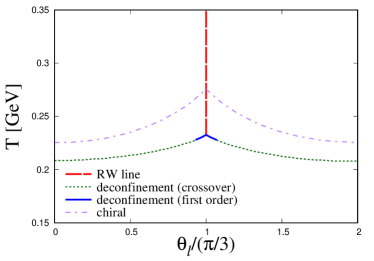
Fig. 4: The phase diagram in the $\theta_{l}$-$T$ plane for condition (I). The dashed line means the RW phase transition line. The crossover (first-order) deconfinement transition line is represented by dotted (solid) line. The dot-dashed line corresponds to the crossover chiral transition line.

At the RW or RW-like phase transition points, $n_{q}$ becomes discontinuous, as already shown in Figs. 2 and 3. This singular behavior is a good indicator to determine the location of the RW or RW-like phase transition points Kouno_JPhys , and we use this property to determine the RW or RW-like phase transition lines. The usefulness of $n_{q}$ to search the RW phase transition point is also discussed from the view point of topological order Kashiwa_holonomy .

Figure 4 presents the QCD phase diagram in the $\theta_{l}$-$T$ plane for condition (I). We only consider the region $\theta_{l}\in[0,2\pi/3]$ because of the RW periodicity. The dot-dashed line is the crossover chiral transition line, and the dotted line is the deconfinement one. The solid line denotes the first-order deconfinement transition line, connected to the endpoint of the RW transition line represented by the dashed line. The RW endpoint is located at $(T^{\rm RW},\theta^{\rm RW}_{l})=(0.233\ \textrm{GeV},\pi/3)$. The chiral transition is crossover in the entire region, while the deconfinement transition becomes first-order, which means that the RW endpoint is a triple point.

We comment on the order of the RW endpoint. The order of deconfinement transition depends on the Polyakov-loop potential $\mathcal{U}$ taken Kouno_JPhys ; Sakai_JPhys and the entanglement coupling $G_{\rm s}(\Phi,\bar{\Phi})$ Sasaki_EPNJL ; Sakai_EPNJL ; Sakai_Sasaki_JPhys . For example, the deconfinement transition becomes second order Kouno_JPhys ; Sakai_JPhys , if we choose

$$\mathcal{U}=-bT\left[54\textrm{e}^{-aT}\Phi\Phi^{\ast}+\log H\right]$$ (30)

as a form of $\mathcal{U}$ Fukushima1 , where $H$ is defined in Eq. (17) and $a,b$ are parameters. In this case, the RW endpoint becomes a tri-critical point. Also in the PNJL model with the entanglement coupling

$$G_{\rm s}(\Phi,\Phi^{\ast})=G_{\rm s}\left(1-\alpha_{1}\Phi\Phi^{\ast}-\alpha_{2}(\Phi^{3}+\Phi^{\ast 3})\right)$$ (31)

and $(\alpha_{1},\alpha_{2})=(0.25,0.1)$, the RW endpoint becomes a tri-critical point Sasaki_EPNJL . This situation requires more robust studies to determine the order of the RW endpoint.

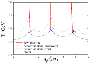
Fig. 5: The phase diagram in the $\theta_{l}$-$T$ plane for condition (II). The meanings of lines are same as in Fig. 5, except that the dashed-line denotes the RW-like phase transition line. Each point of $\textrm{E}_{1}$, $\textrm{E}_{2}$, $\textrm{E}_{3}$ stands for the triple point of the RW-like phase transition line.

Table 2: The location of points $\textrm{E}_{1},\textrm{E}_{2}$ and $\textrm{E}_{3}$ in Fig. 5.

point	$\textrm{E}_{1}$	$\textrm{E}_{2}$	$\textrm{E}_{3}$
$(T,\theta_{l})$	(0.236 GeV, 0.42$\pi$)	(0.246 GeV, $\pi$)	(0.236 GeV, 1.58$\pi$)

Figure 5 is the phase diagram for condition (II). The meaning of lines is the same as in Fig. 4, except that the dashed line denotes the RW-like phase transition line. The location of points $\textrm{E}_{1}$, $\textrm{E}_{2}$ and $\textrm{E}_{3}$ is listed in TABLE 2. The LQCD calculation of Refs. Bonati predicts that the RW-like phase transition occurs at $\theta_{l}\cong 0.45\pi$ for $T=208$ MeV. The PNJL model result $\theta_{l}=0.42\pi$ for $\textrm{E}_{1}$ is consistent with the LQCD value $\theta_{l}\cong 0.45\pi$.

It is found that the RW periodicity is lost, but the phase diagram is line symmetrical with respect to $\theta_{l}=\pi$, because of charge conjugation (C) symmetry of the PNJL model. The symmetry ensures that the chiral transition line has a cusp at point $\textrm{E}_{2}$. Meanwhile, the chiral transition line becomes discontinuous when it hits the RW-like line starting from points $\textrm{E}_{1}$ and $\textrm{E}_{3}$. As for the first-order deconfinement line, it becomes symmetric due to C symmetry around point $\textrm{E}_{2}$, but asymmetric around points $\textrm{E}_{1}$ and $\textrm{E}_{3}$.

In the region $\theta_{l}\in\left[0,2\pi/3\right]$, the RW-like phase transition starts at $\textrm{E}_{1}$, i.e., $(T^{\rm RW^{\prime}},\theta^{\rm RW^{\prime}}_{l})=(0.236\ \textrm{GeV},0.42\pi)$. We fit the transition line by the polynomial function

$$\theta_{l}(n_{\rm max}) =0.42\pi+\sum_{n=1}^{n_{\rm max}}a_{n}\xi^{n},\ \ \xi=\frac{T-T^{\rm RW^{\prime}}}{T^{\rm RW^{\prime}}}.$$ (32)

The transition line is well approximated by $\theta_{l}(n_{\rm max}=3)$ with $a_{1}=-0.023$, $a_{2}=0.93$ and $a_{3}=-1.05$. The smallness of $a_{1}$ means that the line is nearly vertical in the vicinity of $\textrm{E}_{1}$ just as the RW phase transition line, but the transition line deviates from the vertical line as $T$ increases.

The RW-like phase transition line also appears when we consider the imaginary isospin chemical potential $\mu_{I}=i\theta_{I}T$, where $\theta_{I}$ is a dimensionless isospin chemical potential. In the $\theta_{I}$-$T$ plane, the RW-like phase transition line is almost vertical and described by $\theta_{I}=\pi/2-\delta(T)$ with Cea

$$\delta(T)=0.00016\times(T-250).$$ (33)

For the details, see Ref. Sakai_JPhys ; Cea .

In Figs. 4 and 5, the deconfinement transition line joins the RW or RW-like endpoints, and the chiral transition line is higher than the deconfinement one. In LQCD calculation of Ref. Bonati3 , however, the chiral transition line is connected to the endpoints. At the present stage, our model cannot explain the LQCD result. What happens at the endpoints? This is an interesting future work from the theoretical point of view.

Finally, we compare the chiral transition line, $T=T_{\rm c}(\theta_{l})$, calculated by the PNJL model with that by LQCD simulations of Ref. Bonati2 ; note that $\theta_{l}$ varies with $\theta_{s}$ fixed at either 0 or $\theta_{l}$. The ratio $R=T_{\rm c}(\theta_{l})/T_{\rm c}(0)$ is charge-even, and can be parametrized by Bonati ; Bonati2

$$R=1+9\kappa\theta^{2}_{l}+b\theta^{4}_{l}$$ (34)

with the curvature $\kappa$ of the transition line and some constant $b$, when $\theta_{l}$ is not large.

Figure 6 represents $\theta^{2}_{l}$-dependence of $R$ calculated from the PNJL model and LQCD simulations. The PNJL model well reproduces LQCD data for $\theta_{s}=\theta_{l}$ and is almost consistent with LQCD data for $\theta_{s}=0$. Thus, the present PNJL model may be good enough for qualitative analyses.

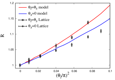
Fig. 6: $\theta^{2}_{l}$-dependence of ratio $R=T_{\rm c}(\theta_{l})/T_{\rm c}(0)$. The horizontal axis is normalized by $\pi^{2}$. The model calculations are represented by solid lines, and data with error bar mean LQCD results Bonati2 .

IV.3 ANALYTICITY OF NUMBER DENSITY

We calculate the imaginary part of up- and strange-quark number densities, $\textrm{Im}\left(n_{u}\right)$ and $\textrm{Im}\left(n_{s}\right)$, by using the PNJL model. We consider the situation that the RW periodicity does not exist, that is, some chemical potentials are fixed to constant values. Only in calculations of $\textrm{Im}\left(n_{u}\right)$, $\theta_{d}$ and $\theta_{s}$ are treated as constants. As for calculations in $\theta_{s}$-dependence of $\textrm{Im}\left(n_{s}\right)$, we again consider $\theta_{u}=\theta_{d}=\theta_{l}$ and these are fixed to constant values.

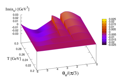
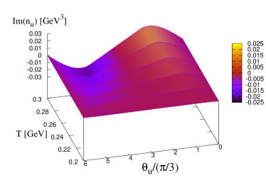
Fig. 7: The $\theta_{u}$- and $T$-dependence of $\textrm{Im}(n_{u})$. The upper panel is the result with $(\theta_{d},\theta_{s})=(\pi/4,0)$, and lower panel is the one with $(\theta_{d},\theta_{s})=(\pi/8,0)$.

Figure 7 shows $\theta_{u}$- and $T$- dependence of $\textrm{Im}(n_{u})$. The upper panel is the result for $(\theta_{d},\theta_{s})=(\pi/4,0)$ and the lower one is for $(\theta_{d},\theta_{s})=(\pi/8,0)$. In the upper panel, $\textrm{Im}(n_{u})$ becomes discontinuous because of the RW-like phase transition, but smooth at any $T$ in the lower panel. We numerically checked that $\textrm{Im}(n_{u})$ becomes smooth at any $T$ when $\theta_{s}=0$ and $\theta_{l}\leq\pi/8$.

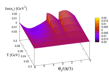
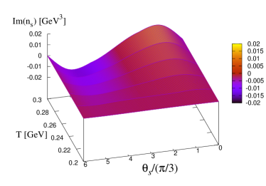
Fig. 8: The $\theta_{s}$- and $T$-dependence of $\textrm{Im}(n_{s})$. The upper panel is the result with $\theta_{l}=\pi/4$, and the lower panel is the one with $\theta_{l}=\pi/5$.

Figure 8 is the result of $\textrm{Im}\left(n_{s}\right)$ as a function of $\theta_{s}$ and $T$. The upper panel corresponds to the result for $\theta_{l}=\pi/4$, and the lower panel is the result for $\theta_{l}=\pi/5$. It is found that the discontinuity of $\textrm{Im}(n_{s})$ disappears for any $T$ when $\theta_{l}=\pi/5$, while $\textrm{Im}(n_{s})$ becomes discontinuous when $\theta_{l}=\pi/4$, due to the RW-like phase transition. We also numerically confirmed that $\textrm{Im}(n_{s})$ has no discontinuity for any $T$ when $\theta_{l}\leq\pi/5$. The results in Fig. 7 (Fig. 8) indicate that $n_{u}$ ($n_{s}$) in the real $\mu_{u}$ ($\mu_{s}$) region can be obtained by the analytic continuation from the imaginary region for any $T$. The present case is thus more informative compared to the case where the RW periodicity exists.

The $n_{\rm s}$ in the high $T$ region plays a key role in determining the strength of the repulsive interaction,

$$\mathcal{L}_{\rm v,s}=-G_{\rm v,s}\left(\bar{s}\gamma^{\mu}s\right)^{2},$$ (35)

where $s$ is the strange-quark field and $G_{\rm v,s}$ is its strength. The behavior of $n_{\rm s}$ is sensitive to the value of $G_{\rm v,s}$, because $n_{\rm s}$ is a function of

$$\tilde{\mu}_{\rm s}=\mu_{\rm s}-2G_{\rm v,s}n_{\rm s}$$ (36)

after the mean-field approximation.

In our previous works Sugano , it was shown that the strength $G_{\rm v}$ of the vector-type four-quark interaction

$$\mathcal{L}_{\rm v}=-G_{\rm v}(\bar{q}\gamma^{\mu}q)^{2}$$ (37)

can be determined from LQCD data on the quark number density $n_{q}$ in the high $T$ region Takahashi2 ; Ejiri . We then pinned down the value of $G_{\rm v}$ from LQCD data on $n_{q}$. However, this analysis did not consider strange quark. Figure 8 indicates that the analytic continuation from imaginary $\mu_{s}$ to real $\mu_{s}$ works well even in the high $T$ region. Thus, one can get reliable $n_{\rm s}$ in both the real- and the imaginary-$\mu_{s}$ region. This allows us to determine the value of $G_{\rm v,s}$ sharply from the LQCD data.

The interaction described by Eq. (35) corresponds to the interaction mediated by $\phi$-meson in the context of the relativistic mean field theory RMF_Glendenning ; RMF_Schaffner ; RMF_Ishizuka ; RMF_Tsubakihara ; RMF_Weissenborn , and affects the maximum mass of neutron star, when the strange quark exists in the inner core of neutron star. It is an interesting future work to investigate the interplay between the $G_{\rm v,s}$ determined from the LQCD data and the maximum mass, and to discuss what happens in the two-solar-mass neutron star Demorest ; Antoniadis .

V SUMMARY

In this paper, we investigated properties of the 2+1-flavor QCD in the imaginary chemical potential region with finite $\mu_{l}=i\theta_{l}T$ and $\mu_{s}=i\theta_{s}T$, using two approaches. One is a theoretical approach based on the QCD partition function, and the other is a qualitative one based on an effective model. In the theoretical approach, we proved that the QCD thermodynamic potential $\Omega_{\rm QCD}$ exhibits the Roberge-Weiss (RW) periodicity only when $\Omega_{\rm QCD}$ is invariant under the extended $\mathbb{Z}_{3}$ transformation. In other words, the RW periodicity disappears when two chemical potentials are fixed to a constant value. Next, we showed that the thermodynamic potential of the Polyakov-loop extended Nambu–Jona-Lasinio (PNJL) model also possesses the extended $\mathbb{Z}_{3}$ symmetry. We then took the PNJL model as a useful effective model.

Taking the PNJL model, we calculated $\Omega_{\rm PNJL}$, $\textrm{Im}\left(n_{q}\right)$ (the imaginary part of quark number density), and the QCD phase diagram as a function of $\theta_{l}$ for two conditions; (I) $\theta_{s}=\theta_{l}$ and (II) $\theta_{s}=0$. For condition (I), the RW periodicity is seen in all the results. The structure of the phase diagram is similar to the one in 2-flavor case Sakai_JPhys . As for condition (II), there is no RW periodicity, but we found that the region available for the analytic continuation is broader than condition (I). The noteworthy points on the phase diagram are the following:

1. The crossover chiral transition line becomes discontinuous on the RW-like phase transition line,

2. The first-order deconfinement transition line is asymmetric with respect to the RW-like phase transition line, except for at $\theta_{l}=\pi$.

3. The first-order RW-like phase transition line can be well fitted by a polynomial function of Eq. (32) with $n_{\rm max}=3$.

Finally, we calculated the imaginary part of up- and strange-quark number densities, $\textrm{Im}(n_{u})$ and $\textrm{Im}(n_{s})$. We consider the situation that two of chemical potentials are fixed to constant values and thereby the RW periodicity disappears. When $\theta_{s}=0$ and $\theta_{d}\leq\pi/8$, $\textrm{Im}(n_{u})$ becomes an analytic function of $\theta_{u}$ for any $T$. The condition for $\textrm{Im}\left(n_{s}\right)$ to be an analytic function of $\theta_{s}$ for any $T$ is $\theta_{u}=\theta_{d}=\theta_{l}\leq\pi/5$. When these conditions are satisfied, the values of $n_{u}$ and $n_{s}$ can be calculated by the analytic continuation, for any $T$ of interest.

In the present paper, we concentrate on qualitative discussion based on the extended $\mathbb{Z}_{3}$ symmetry. The results mentioned above are interesting theoretically, but do not exactly correspond to the realistic case. As a future work, it is quite interesting to make systematic and quantitative analyzes, particularly in more realistic cases.

- (1) M. Stephanov, arXiv:0701002.
- (2) P. Braun-Munzinger and J. Wambach, Rev. Mod. Phys. 81, 1031 (2009).
- (3) K. Fukushima and T. Hatsuda, Rept. Prog. Phys. 74, 014001 (2011).
- (4) K. Fukushima and C. Sasaki, Prog. Part. Nucl. Phys. 72, 99 (2013).
- (5) P. de Forcrand and O. Philipsen, Nucl. Phys. B642, 290 (2002).
- (6) M. D’Elia and M. P. Lombardo, Phys. Rev. D 67, 014505 (2003).
- (7) L. K. Wu, X. Q. Luo, and H. S. Chen, Phys. Rev. D 76, 034505.
- (8) M. D’Elia and F. Sanfilippo, Phys. Rev. D 80, 111501 (2009).
- (9) P. de Forcrand and O. Philipsen, Phys. Rev. Lett. 105, 152001 (2010).
- (10) K. Nagata and A. Nakamura, Phys. Rev. D 83, 114507 (2011).
- (11) P. Cea, L. Cosmai, M. D’Elia, A. Papa, and F. Sanfilippo, Phys. Rev. D 85, 094512 (2012).
- (12) J. Takahashi, K. Nagata, T. Saito, A. Nakamura, T. Sasaki, H. Kouno, and M. Yahiro, Phys. Rev. D 88, 114504 (2013).
- (13) C. Bonati, P. de Forcrand, M. D’Elia, O. Philipsen, and F. Sanfilippo, Phys. Rev. D 90, 074030 (2014).
- (14) J. Takahashi, H. Kouno, and M. Yahiro, Phys. Rev. D 91, 014501 (2015).
- (15) A. Roberge and N. Weiss, Nucl. Phys. B275, 734 (1986)
- (16) P. N. Meisinger and M. C. Ogilvie, Phys. Lett. B379, 163 (1996).
- (17) A. Dumitru, and R. D. Pisarski, Phys. Rev. D 66, 096003 (2002).
- (18) K. Fukushima, Phys. Lett. B591, 277 (2004); Phys. Rev. D 77, 114028 (2008); Phys. Rev. D 78, 114019 (2008).
- (19) S. K. Ghosh, T. K. Mukherjee, M. G. Mustafa, and R. Ray, Phys. Rev. D 73, 114007 (2006).
- (20) E. Megías, E. R. Arriola, and L. L. Salcedo, Phys. Rev. D 74, 065005 (2006).
- (21) C. Ratti, M. A. Thaler, and W. Weise, Phys. Rev. D 73, 014019 (2006).
- (22) S. Rößner, C. Ratti, and W. Weise, Phys. Rev. D 75, 034007 (2007).
- (23) K. Kashiwa, H. Kouno, M. Matsuzaki, and M. Yahiro, Phys. Lett. B662, 26 (2008).
- (24) Y. Sakai, K. Kashiwa, H. Kouno, and M. Yahiro, Phys. Rev. D 77, 051901(R) (2008).
- (25) Y. Sakai, K. Kashiwa, H. Kouno, and M. Yahiro, Phys. Rev. D 78, 036001 (2008).
- (26) Y. Sakai, K. Kashiwa, H. Kouno, M. Matsuzaki, and M. Yahiro, Phys. Rev. D 78, 076007 (2008).
- (27) Y. Sakai, K. Kashiwa, H. Kouno, M. Matsuzaki, and M. Yahiro, Phys. Rev. D 79, 096001 (2009).
- (28) Y. Sakai, H. Kouno, and M. Yahiro, J. Phys. G 37, 105007 (2010).
- (29) P. Cea, L. Cosmai, M. D’Elia, C. Manneschi, and A. Papa, Phys. Rev. D 80, 034501 (2009).
- (30) C. Bonati, M. D’Elia, M. Mariti, M. Mesiti, F. Negro, and F. Sanfilippo, Phys. Rev. D 90, 114025 (2014).
- (31) C. Bonati, M. D’Elia, M. Mariti, M. Mesiti, F. Negro, and F. Sanfilippo, Phys. Rev. D 92, 054503 (2015).
- (32) C. Bonati, M. D’Elia, M. Mariti, M. Mesiti, F. Negro, and F. Sanfilippo, Phys. Rev. D 93, 074504 (2016).
- (33) M. D’Elia, G. Gagliardi, and F. Sanfilippo, arXiv:1611.08285.
- (34) G. Boyd, J. Engels, F. Karsch, E. Laermann, C. Legeland, M. Lütgemeire, and B. Petersson, Nucl. Phys. B469, 419 (1996).
- (35) O. Kaczmarek, F. Karsch, P. Petreczky, and F. Zantow, Phys. Lett. B543, 41 (2002).
- (36) E. Laermann and O. Philipsen, Annu. Rev. Nucl. Part. Sci. 53, 163 (2003).
- (37) Z. Fodor and S. D. Katz, arXiv:0908.3341 (2009).
- (38) S. Borsányi, Z. Fodor, C. Hoelbling, S. D. Katz, S. Krieg, C. Ratti, and K. K. Szabo, J. High Energy Phys. 09 (2010) 073.
- (39) W. Söldner, arXiv:1012.4484.
- (40) K. Kanaya, AIP Conf. Proc. 1343, 57 (2011); arXiv:1012.4247.
- (41) T. Sasaki, Y. Sakai, H. Kouno, and M. Yahiro, Phys. Rev. D 84, 091901(R) (2011).
- (42) G. ’t Hooft, Phys. Rev. Lett. 37, 8 (1976); Phys. Rev. D 14, 3432 (1976).
- (43) M. Kobayashi and T. Maskawa, Prog. Theor. Phys. 44, 1422 (1970).
- (44) M. Kobayashi, H. Kondo, and T. Maskawa, Prog. Theor. Phys. 45, 1955 (1971).
- (45) P. Rehberg, S. P. Klevansky, and J. Hüfner, Phys. Rev. C 53, 410 (1996).
- (46) S. P. Klevansky, Rev. Mod. Phys. 64, 649 (1992).
- (47) H. Kouno, Y. Sakai, K. Kashiwa, and M. Yahiro, J. Phys. G 36, 115010 (2009).
- (48) C. Sasaki, B. Friman, and K. Redlich, Phys. Rev. D 75, 074013 (2007).
- (49) K. Kashiwa and A. Ohnishi, Phys. Lett. B750, 282 (2015); Phys. Rev. D 93, 116002 (2016); arXiv:1701.04953.
- (50) Y. Sakai, T. Sasaki, H. Kouno, and M. Yahiro, Phys. Rev. D 82, 076003 (2010).
- (51) Y. Sakai, T. Sasaki, H. Kouno, and M. Yahiro, J. Phys. G 39, 035004 (2012).
- (52) J. Sugano, J. Takahashi, M. Ishii, H. Kouno, and M. Yahiro, Phys. Rev. D 90, 037901 (2014); J. Sugano, H. Kouno, and M. Yahiro, Phys. Rev. D 94, 014024 (2016).
- (53) S. Ejiri, Y. Maezawa, N. Ukita, S. Aoki, T. Hatsuda, N. Ishii, K. Kanaya, and T. Umeda, Phys. Rev. D 82, 014508 (2010).
- (54) N. K. Glendenning, Phys. Lett. B114, 392 (1982).
- (55) J. Schaffner and I. N. Mishustin, Phys. Rev. C 53, 1416 (1996).
- (56) C. Ishizuka, A. Ohnishi, K. Tsubakihara, K. Sumiyoshi, and S. Yamada, J. Phys. G 35, 085201 (2008).
- (57) K. Tsubakihara, H. Maekawa, H. Matsumiya, and A. Ohnishi, Phys. Rev. C 81, 065206 (2010); K. Tsubakihara, A. Ohnishi, and T. Harada, arXiv:1402.0979.
- (58) S. Weissenborn, D. Chatterjee, and J. Schaffner-Bielich, Nucl. Phys. A881, 62 (2012); Phys. Rev. C 85, 065802 (2012); Nucl. Phys. A914, 421 (2013).
- (59) P. B. Demorest, T. Pennucci, S. M. Ransom, M. S. E. Roberts, and J. W. T. Hessels, Nature (London) 467, 1081 (2010).
- (60) J. Antoniadis et al., Science 340, 1233232 (2013).