Lower Bounds on Exponential Moments of the Quadratic Error in Parameter Estimation

Abstract

Considering the problem of risk–sensitive parameter estimation, we propose a fairly wide family of lower bounds on the exponential moments of the quadratic error, both in the Bayesian and the non–Bayesian regime. This family of bounds, which is based on a change of measures, offers considerable freedom in the choice of the reference measure, and our efforts are devoted to explore this freedom to a certain extent. Our focus is mostly on signal models that are relevant to communication problems, namely, models of a parameter–dependent signal (modulated signal) corrupted by additive white Gaussian noise, but the methodology proposed is also applicable to other types of parametric families, such as models of linear systems driven by random input signals (white noise, in most cases), and others. In addition to the well known motivations of the risk–sensitive cost function (i.e., the exponential quadratic cost function), which is most notably, the robustness to model uncertainty, we also view this cost function as a tool for studying fundamental limits concerning the tail behavior of the estimation error. Another interesting aspect, that we demonstrate in a certain parametric model, is that the risk–sensitive cost function may be subjected to phase transitions, owing to some analogies with statistical mechanics.

Index Terms: risk–sensitive estimation, risk–averse estimation, robust estimation, Bayesian estimation, Cramér–Rao bound, unbiased estimation, tail behavior, phase transitions.

1 Introduction

While the minimum mean square error (MMSE) has been the most common figure of merit for measuring the performance of estimators in several areas, such as estimation theory, information/communication theory, and statistics, by contrast, the exponential moments of the quadratic error, namely, $\mbox{\boldmath$E$}\exp\{\alpha(\hat{\theta}-\theta)^{2})\}$ ($\alpha>0$ being a prescribed constant, $\theta$ – a parameter, and $\hat{\theta}$ – its estimator), have received much less attention in those fields. In the realm of the theory of optimization and stochastic filtering and control, on the other hand, the problem of minimizing exponential moments of the quadratic error, or exponential moments of any other loss function, has been studied rather intensively, and it is well–known as the risk–sensitive or risk–averse cost function (see, e.g., [8], [10], [13], [18], [30], [31] and many references therein).

One of the main motivations for using the exponential function of the loss is to impose a penalty, or a risk, that is extremely sensitive to large values of the loss, hence the qualifier “risk–sensitive” in the name of this criterion. Another motivation is associated with robustness properties of the resulting risk–sensitive solutions to model uncertainties [1], [12]. Indeed, as explained in [22, p. 349, the paragraph of eq. (11)], minimization of the exponential moment of the loss function is equivalent to minimization of the expected loss for the worst distribution in the $\epsilon$–neighborhood (in the Kullback–Leibler divergence sense) of the given (nominal) probability distribution, where $\epsilon$ grows with the risk–sensitive factor parameter $\alpha$. There are, in fact, a few additional motivations for minimizing exponential moments, which are also relevant to the problem of parameter estimation considered here, and indeed, risk–sensitive parameter estimation has been studied to a considerable extent (see, e.g., [3], [14], [17], [19], [24], [25], [26], [32], and references therein). First and foremost, the exponential moment, $\mbox{\boldmath$E$}\exp\{\alpha(\hat{\theta}-\theta)^{2}\}$, as a function of $\alpha$, is obviously the moment–generating function of $(\hat{\theta}-\theta)^{2}$, and as such, it provides the full information about the entire distribution of this random variable, not just its first order moment. Thus, in particular, if we are fortunate enough to find an estimator that uniformly minimizes $\mbox{\boldmath$E$}\exp\{\alpha(\hat{\theta}-\theta)^{2}\}$ for all $\alpha\geq 0$ (and there are examples that this may be the case), then this is much stronger than just minimizing the first moment. Secondly, exponential moments are intimately related to large–deviations rate functions (owing to the exponential tightness of the Chernoff bound), and so, the minimization of exponential moments may give us an edge on minimizing probabilities of (undesired) large deviations events of the form $\mbox{Pr}\{|\hat{\theta}-\theta|\geq\delta\}$ (for some threshold $\delta$ which is related to $\alpha$), or more precisely, on maximizing the exponential rate of decay of these probabilities.

Moreover, an important feature of the estimation error, $\epsilon\equiv\hat{\theta}-\theta$, is its tail behavior: how fast can the probability density function (pdf) of $\epsilon$ possibly decay as $|\epsilon|\to\infty$ (assuming the support of $\epsilon$ to be unbounded)? This is not accomplished, in general, by inspecting a figure of merit like $\mbox{Pr}\{|\hat{\theta}-\theta|\geq\delta\}$, for a given $\delta$, since the optimal estimator under this criterion may depend on $\delta$, whereas we might be interested to assess the decay rate of the entire distribution tail of a single estimator $\hat{\theta}$. It turns out that when the support of $\theta$ is unbounded (and so is that of $\hat{\theta}$), then there is normally a critical value of $\alpha$, denoted $\alpha_{\mbox{\tiny c}}$, such that for every $\alpha<\alpha_{\mbox{\tiny c}}$, the exponential moment $\mbox{\boldmath$E$}\exp\{\alpha(\hat{\theta}-\theta)^{2}\}$ is finite at least for some estimators, whereas, for $\alpha\geq\alpha_{\mbox{\tiny c}}$, it must diverge for any estimator $\hat{\theta}$. When this is the case, this means that there exists no estimator whose pdf tail decays faster than a Gaussian tail of the form $\exp(-\alpha_{\mbox{\tiny c}}\epsilon^{2})$. Thus, deriving bounds on $\alpha_{\mbox{\tiny c}}$ is an important aspect of the risk–sensitive cost function, as we shall see in the sequel. Interestingly, in a large variety of models that we examine, our bounds on $\alpha_{\mbox{\tiny c}}$ will turn out to be tight in spite of the fact that the corresponding bounds to the mean exponential quadratic error are not always tight.

Our main focus in this paper is in lower bounds to the mean exponential quadratic error as a function of the risk–sensitive parameter $\alpha$. We propose a rather wide family of such lower bounds, both in the Bayesian and non–Bayesian regimes, though most of our emphasis is on the Bayesian regime. This family of bounds is based on a change of measures, combined with the plethora of bounds for the ordinary mean square error (MSE), and as such, it offers a considerably large freedom in the choice of certain ingredients of these bounds. Our efforts are devoted to explore this freedom at least to a certain extent. The bounds are applied mostly to signal models that are relevant to communication problems, namely, models of a parameter–dependent signal (i.e., a modulated signal) corrupted by additive white Gaussian noise, but the methodology proposed is also applicable to other types of parametric families, such as models of linear systems driven by random input signals (white noise, in most cases), memoryless sources parametrized by their letter probabilities, Markov sources, parametrized by their state transition probabilities, and so on. Another interesting aspect, that we demonstrate (in the Bayesian regime) for a very simple parametric model, is that the risk–sensitive cost function may be subjected to phase transitions, owing to some intimate analogies with statistical mechanics.

The remaining part of this paper is organized as follows. In Section 2, we establish notation conventions, define the problem, and provide a few preliminaries. In Section 3, we provide our generic lower bounds to the risk–sensitive cost function for both the Bayesian and the non–Bayesian regimes. These two generic bounds will serve as the basis for several families of bounds that will be further developed for various classes of parametric models in Section 4 (the Bayesian regime) and in Section 5 (the non–Bayesian regime). Also, in the last subsection of Section 4, we demonstrate that the risk–sensitive cost function may exhibit phase transitions even in some simple parametric models, like that of the binary memoryless (Bernoulli) source.

2 Notation, Definitions, Problem Setting and Preliminaries

We begin by establishing some notation conventions. We consider a parametric family of probability functions, $\{P(\mbox{\boldmath$y$}|\theta),~{}\theta\in{\cal A}\}$, where $\theta$ is parameter taking values in a parameter set ${\cal A}$, and $y$ is a set of observations. For the sake of simplicity of the presentation, throughout most of of this paper, $\theta$ will be a scalar parameter, and accordingly, ${\cal A}$ will be either an interval, or half of the real line, or the entire real line. In a few places along the paper, however, we will let $\theta$ be a vector of finite dimension $k$ and accordingly, ${\cal A}$ will be ${\rm I\!R}^{k}$ or a subset of it. The set of observations, $y$, may either be a vector of dimension $n$, $\mbox{\boldmath$y$}=(y_{1},\ldots,y_{n})$ (in the discrete–time case) or a waveform $\mbox{\boldmath$y$}=\{y(t),~{}0\leq t\leq T\}$ (in the continuous–time, Gaussian case), depending on the context. In the latter case, the conditional pdf $P(\mbox{\boldmath$y$}|\theta)$ will be understood to be defined via a complete family of orthonormal basis functions, according to the well known conventions (see, e.g., [16, Chap. 8]). In the Bayesian setting, we will assume that $\theta$ is a random variable, distributed according to a given prior $P(\theta)$, whose support is ${\cal A}$. The joint density of $\theta$ and $y$ will then be given by $P(\theta,\mbox{\boldmath$y$})=P(\theta)P(\mbox{\boldmath$y$}|\theta)$. Alternative joint densities of $\theta$ and $y$ will be denoted by the letter $Q$ (e.g., $Q(\theta)$, $Q(\mbox{\boldmath$y$}|\theta)$, etc.).

An estimator, $\hat{\theta}$, of the parameter $\theta$, is any measurable function of $y$ only. Following customary notation conventions, we will use capital letters to designate randomness. Accordingly, $Y$ will denote the random observation set, and in the Bayesian setting $\Theta$ will denote a random parameter governed by the prior $P(\theta)$.

In the non–Bayesian setting, where $\theta$ is assumed an unknown deterministic variable, $P_{\theta}\{{\cal E}\}$ will denote the probability of an event ${\cal E}$, associated with $Y$, under $P(\cdot|\theta)$, and similarly, $\mbox{\boldmath$E$}_{\theta}\{f(\mbox{\boldmath$Y$})\}$ will denote the expectation of some function $f$ of the random observation set $Y$, with respect to (w.r.t.) $P(\cdot|\theta)$. An estimator $\hat{\theta}\equiv\hat{\theta}(\mbox{\boldmath$y$})$ is called unbiased if for every $\theta\in{\cal A}$, we have $\mbox{\boldmath$E$}_{\theta}\hat{\theta}=\theta$. The Kullback–Leibler divergence between the conditional densities $P_{\tilde{\theta}}=P(\cdot|\tilde{\theta})$ and $P_{\theta}=P(\cdot|\theta)$ will be defined as

$$D(P_{\tilde{\theta}}\|P_{\theta})=\mbox{\boldmath$E$}_{\tilde{\theta}}\ln\frac{P(\mbox{\boldmath$Y$}|\tilde{\theta})}{P(\mbox{\boldmath$Y$}|\theta)},$$ (1)

provided that the support of $P(\cdot|\tilde{\theta})$ covers the one of $P(\cdot|\theta)$.

In the Bayesian setting, the probability of an event ${\cal E}$, associated with $Y$ and $\Theta$, will be denoted by $P\{{\cal E}\}$ and the expectation of a given function $f(\mbox{\boldmath$Y$},\Theta)$, will be denoted by $\mbox{\boldmath$E$}\{f(\mbox{\boldmath$Y$},\Theta)\}$. The conditional expectation of $f(\mbox{\boldmath$Y$},\Theta)$ given $\mbox{\boldmath$Y$}=\mbox{\boldmath$y$}$ (which is the same as the conditional expectation of $f(\mbox{\boldmath$y$},\Theta)$) will be denoted by $\mbox{\boldmath$E$}\{f(\mbox{\boldmath$y$},\Theta)|\mbox{\boldmath$y$}\}$. Expectations and conditional expectations w.r.t. an alternative joint density $\{Q(\theta,\mbox{\boldmath$y$})\}$ will be subscripted by $Q$, i.e., $\mbox{\boldmath$E$}_{Q}\{f(\Theta,\mbox{\boldmath$Y$})\}$, $\mbox{\boldmath$E$}_{Q}\{f(\Theta,\mbox{\boldmath$y$})|\mbox{\boldmath$y$}\}$, etc. The Kullback–Leibler divergence between $Q$ and $P$ will be defined as

$$D(Q\|P)=\mbox{\boldmath$E$}_{Q}\ln\frac{Q(\Theta,\mbox{\boldmath$Y$})}{P(\Theta,\mbox{\boldmath$Y$})},$$ (2)

provided that the support of $Q$ covers the support of $P$.

In this paper, we judge the performance of any estimator according to the exponential moment of the squared error, henceforth referred to as the risk–sensitive cost function, which is parametrized by a positive real $\alpha$, called the risk–sensitive factor, and is defined as follows. In the non–Bayesian regime,

$$\Lambda_{\mbox{\tiny NB}}(\hat{\theta},\theta,\alpha)\stackrel{{\scriptstyle\Delta}}{{=}}\ln\mbox{\boldmath$E$}_{\theta}\left\{\exp\left(\alpha[\hat{\theta}(\mbox{\boldmath$Y$})-\theta]^{2}\right)\right\},$$ (3)

with the quest of minimizing $\Lambda_{\mbox{\tiny NB}}$ over all unbiased estimators, uniformly for all $\theta\in{\cal A}$. In the Bayesian regime, the risk–sensitive cost function is defined as

$$\Lambda_{\mbox{\tiny B}}(\hat{\theta},\alpha)\stackrel{{\scriptstyle\Delta}}{{=}}\ln\mbox{\boldmath$E$}\left\{\exp\left(\alpha[\hat{\theta}(\mbox{\boldmath$Y$})-\Theta]^{2}\right)\right\},$$ (4)

with the quest of minimizing $\Lambda_{\mbox{\tiny B}}$ over all estimators in general. The risk–sensitive factor, $\alpha$, controls the degree of risk–sensitivity, or the degree of robustness of the estimator that minimizes the risk–sensitive cost function. The larger is $\alpha$, the greater is the sensitivity to large errors. The limit $\alpha\to 0$ recovers the case of ordinary MSE estimation.

It should be pointed out that even in the Bayesian regime (let alone the non–Bayesian one), the optimal estimator

$$\hat{\theta}=\mbox{arg}\min_{\eta}\mbox{\boldmath$E$}\{e^{\alpha(\Theta-\eta)^{2}}|\mbox{\boldmath$y$}\}$$ (5)

is not trivial to calculate, in general, as it is associated with the solution $\eta$ of the equation

$$\eta=\frac{\mbox{\boldmath$E$}\{\Theta e^{\alpha(\Theta-\eta)^{2}}|\mbox{\boldmath$y$}\}}{\mbox{\boldmath$E$}\{e^{\alpha(\Theta-\eta)^{2}}|\mbox{\boldmath$y$}\}},$$ (6)

which cannot be solved in closed–form in most cases. This is even more difficult than calculating the MMSE estimator, i.e., the conditional expectation, $\mbox{\boldmath$E$}\{\Theta|\mbox{\boldmath$y$}\}$, which is known to be a non–trivial task (if not completely undoable) on its own right, in the vast majority of cases of practical interest. Thus, the need for good lower bounds to $\Lambda_{\mbox{\tiny NB}}(\hat{\theta},\theta,\alpha)$ and $\Lambda_{\mbox{\tiny B}}(\hat{\theta},\alpha)$ is at least as crucial as in the classical case of the MSE cost function.

3 Generic Lower Bounds

Our basic, generic lower bounds, for both the Bayesian and the non–Bayesian regimes, are provided in the following theorem, whose very simple proof appears at the end of this section.

Theorem 1

Consider the parametric family defined in Section 2.

1. For every estimator $\hat{\theta}$,

   $$\Lambda_{\mbox{\tiny B}}(\hat{\theta},\alpha)\geq\alpha L_{\mbox{\tiny B}}(Q)-D(Q\|P),$$ (7)

   where $Q$ is an arbitrary joint density of $(\Theta,\mbox{\boldmath$Y$})$ and $L_{\mbox{\tiny B}}(Q)$ is an arbitrary lower bound to $\mbox{\boldmath$E$}_{Q}[\hat{\theta}(\mbox{\boldmath$Y$})-\Theta]^{2}$.

2. For every unbiased estimator $\hat{\theta}$,

   $$\Lambda_{\mbox{\tiny NB}}(\hat{\theta},\theta,\alpha)\geq\alpha L_{\mbox{\tiny NB}}(\tilde{\theta})+\alpha(\tilde{\theta}-\theta)^{2}-D(P_{\tilde{\theta}}\|P_{\theta}),$$ (8)

   where $\tilde{\theta}$ is an arbitrary parameter value in ${\cal A}$ and $L_{\mbox{\tiny NB}}(\tilde{\theta})$ is any non–Bayesian lower bound on the MSE, $\mbox{\boldmath$E$}_{\tilde{\theta}}(\hat{\theta}-\tilde{\theta})^{2}$, for unbiased estimators.

As can be seen, both generic bounds offer a rather wide spectrum of choices with many degrees of freedom. In the Bayesian lower bound (part 1 of Theorem 1), one has the freedom to choose both the joint density $Q$, henceforth referred to as the reference model, and the MSE lower bound, $L_{\mbox{\tiny B}}(Q)$. As for the former, since the inequality (7) applies for any $Q$, one has the freedom to select the one that maximizes the r.h.s. of (7) over a certain class ${\cal Q}$ of reference models, and it would be wise to define the class ${\cal Q}$ to be wide enough to yield good bounds, on the one hand, and structured enough to make the problem of maximization over ${\cal Q}$ tractable, on the other hand. First and foremost, ${\cal Q}$ should be a family of other parametric models for which it is relatively easy to derive a good lower bound, $L_{\mbox{\tiny B}}(Q)$ (or even the exact MMSE), as well as an expression (or at least an upper bound) to $D(Q\|P)$. Of course, the choice $Q=P$ is always legitimate, but it normally leads to a rather trivial lower bound – the same bound that is obtained by a simple application of the Jensen inequality ($\ln\mbox{\boldmath$E$}e^{Z}\geq\mbox{\boldmath$E$}Z$), which is a relatively weak bound in most cases. Of course, if ${\cal Q}$ is chosen to include $P$ as a member, the bound resulting from maximization over ${\cal Q}$ cannot be worse than this trivial lower bound. The MSE lower bound, $L_{\mbox{\tiny B}}(Q)$, can chosen, for example, to be the Bayesian Cramér–Rao bound [27], or the Weiss–Weinstein lower bound [29], or any one of their many variants, see, e.g., [28] and many references therein.

Similar comments apply to the non–Bayesian setting (part 2 of Theorem 1). Here the degrees of freedom are in the selection of the reference parameter value, $\tilde{\theta}$, and in the selection of the non–Bayesian MSE lower bound, $L_{\mbox{\tiny NB}}(\tilde{\theta})$. The best choice of $\tilde{\theta}$ is, of course, the one that maximizes the r.h.s. of (8) over ${\cal A}$, but this maximization is not always an easy task. The MSE lower bound, $L_{\mbox{\tiny NB}}(\tilde{\theta})$, can be taken to be one of many existing non–Bayesian lower bounds for unbiased estimators, for example, the non–Bayesian Cramér–Rao lower bound (see, e.g., [27]), the Bhattacharyya bound [4], the Chapman–Robbins bound [6], the Fraser–Guttman bound [15], the Barankin bound [5], the Keifer bound [20], etc.

We note that when the support ${\cal A}$ of the parameter $\theta$ is unbounded, the maximization of the lower bound (over $Q\in{\cal Q}$ – in the Bayesian case, or over $\tilde{\theta}\in{\cal A}$ – in the non–Bayesian case) might yield an infinite value for large enough $\alpha$, say, for every $\alpha\geq\alpha_{\mbox{\tiny c}}$, where $\alpha_{\mbox{\tiny c}}$ is referred to as the critical value of $\alpha$. When this is the case, it means that the pdf of the estimation error, $\epsilon\stackrel{{\scriptstyle\Delta}}{{=}}\hat{\theta}-\theta$, decays at a rate slower than $\exp\{-\alpha_{\mbox{\tiny c}}\epsilon^{2}\}$ for $|\epsilon|\to\infty$. The lower bounds of Theorem 1 can therefore yield upper bounds to $\alpha_{\mbox{\tiny c}}$. If $\alpha_{\mbox{\tiny c}}=0$, it means that there is no estimator with an estimation error whose tail decays as fast as any Gaussian. We will encounter situations where this is indeed the case: interestingly, while for many estimators, the error is nearly Gaussian around the origin (due to an underlying central limit theorem), the tails may decay at a much slower rate than any Gaussian tail. In the other extreme, if $\alpha_{\mbox{\tiny c}}=\infty$, which is the case where the lower bound is finite no matter how large $\alpha$ may be, the tail of the error may decay faster than any Gaussian. Of course, when ${\cal A}$ is a finite interval, this is trivially the case. We shall comment on the behavior of $\alpha_{\mbox{\tiny c}}$ in the various cases that we consider.

Some of the resulting bounds (Bayesian and non–Bayesian alike) can easily be extended to the vector case. Considering, for example, the risk–sensitive cost function

$$\Lambda_{\mbox{\tiny NB}}(\hat{\theta},\theta,\alpha)=\ln\mbox{\boldmath$E$}_{\theta}\exp\left\{[\alpha^{T}(\hat{\theta}-\theta)]^{2}\right\},$$ (9)

where $\alpha$ is $\theta$ are now both column vectors of dimension $k$ and the superscript $T$ denotes transposition, the above quantity is readily lower bounded by

$$\alpha^{T}[I^{-1}(\tilde{\theta})+(\tilde{\theta}-\theta)(\tilde{\theta}-\theta)^{T}]\alpha-D(P_{\tilde{\theta}}\|P_{\theta}),$$ (10)

where $I^{-1}(\tilde{\theta})$ is the inverse of the $k\times k$ Fisher information matrix associated with the parametric family $\{P(\cdot|\theta),~{}\theta\in{\cal A}\}$. This gives some fundamental limitations on arbitrary projections of the estimation error as well as on the behavior of the tails of the estimation error in various directions in ${\rm I\!R}^{k}$.

In the remaining part of this paper, we shall make an attempt to explore some of these degrees of freedom. Most of our efforts will be given to the Bayesian regime, but we will also devote some attention to the Bayesian regime. We end this section by providing the proof of Theorem 1.

Proof of Theorem 1. We begin from a very simple well–known inequality, which stands at the basis of the Laplace principle [11] or more generally, the Varadhan integral lemma [9, Section 4.3]. Let $Z$ be a random variable, governed by a probability distribution $P$, and let $Q$ be an alternative probability distribution on the same space, such that $D(Q\|P)<\infty$. Now,

$$\ln\mbox{\boldmath$E$}_{P}e^{Z}=\ln\mbox{\boldmath$E$}_{Q}\exp\left\{Z+\ln\frac{P(Z)}{Q(Z)}\right\}\geq\mbox{\boldmath$E$}_{Q}Z-D(Q\|P),$$ (11)

where the second step follows from the Jensen inequality.

Next apply eq. (11) to both the Bayesian and the non–Bayesian regime. For the Bayesian regime, set $Z=\alpha[\hat{\theta}(\mbox{\boldmath$Y$})-\Theta]^{2}$, then further lower bound $\mbox{\boldmath$E$}_{Q}[\hat{\theta}(\mbox{\boldmath$Y$})-\Theta]^{2}$ by $L_{\mbox{\tiny B}}(Q)$, which will yield part 1 of Theorem 1. For the non–Bayesian regime (part 2 of Theorem 1), set $Z=[\hat{\theta}(\mbox{\boldmath$Y$})-\theta]^{2}$, use $P_{\theta}$ in the role of $P$, $P_{\tilde{\theta}}$ – in the role of $Q$, and then further lower bound $\mbox{\boldmath$E$}_{\tilde{\theta}}(\hat{\theta}-\theta)^{2}$ by

$$\mbox{\boldmath$E$}_{\tilde{\theta}}(\hat{\theta}-\theta)^{2}=\mbox{\boldmath$E$}_{\tilde{\theta}}(\hat{\theta}-\tilde{\theta})^{2}+(\tilde{\theta}-\theta)^{2}\geq L_{\mbox{\tiny NB}}(\tilde{\theta})+(\tilde{\theta}-\theta)^{2},$$ (12)

where in the first step, we have used the assumed unbiasedness of $\hat{\theta}$ and in the second step, we have used the definition of $L_{\mbox{\tiny NB}}(\tilde{\theta})$. This completes the proof of Theorem 1.

4 The Bayesian Regime

4.1 Conditions for Tightness of the Lower Bound

Before exploring the lower bound of the Bayesian regime in specific parametric models, we would like first to furnish conditions under which this bound is tight. Applying Observation 1 of [22, p. 347] to Bayesian parameter estimation, we find that an estimator $\hat{\theta}$ minimizes $\Lambda_{\mbox{\tiny B}}(\hat{\theta},\alpha)$ if it also minimizes $\mbox{\boldmath$E$}_{Q}(\hat{\theta}-\Theta)^{2}$, where $Q(\theta|\mbox{\boldmath$y$})$ is given by

$$Q(\theta|\mbox{\boldmath$y$})=\frac{P(\theta|\mbox{\boldmath$y$})e^{\alpha[\hat{\theta}(\mbox{\boldmath$y$})-\theta]^{2}}}{Z(\mbox{\boldmath$y$})},$$ (13)

and where $Z(\mbox{\boldmath$y$})$ is a normalization constant, so that $Q(\cdot|\mbox{\boldmath$y$})$ would integrate to unity. In other words, to minimize $\Lambda_{\mbox{\tiny B}}(\hat{\theta},\alpha)$, the estimator $\hat{\theta}$ has to be the conditional expectation of $\Theta$ given $y$ w.r.t. $Q$. Note that this condition has a circular character, since $Q$ depends on $\hat{\theta}$, which in turn depends on $Q$. Therefore, this condition for optimality is more useful as a criterion to check whether a given estimator is optimal than as a tool for actually finding the optimal estimator. Further, let us lower bound $\mbox{\boldmath$E$}_{Q}(\hat{\theta}-\Theta)^{2}$ by $L_{\mbox{\tiny B}}(Q)$, which is given by the Bayesian Cramér–Rao lower bound [27] w.r.t. $Q$, that is,

$$L_{\mbox{\tiny B}}(Q)=\frac{1}{\mbox{\boldmath$E$}_{Q}W^{2}(\Theta,\mbox{\boldmath$Y$})},$$ (14)

where

$$W(\theta,\mbox{\boldmath$y$})\stackrel{{\scriptstyle\Delta}}{{=}}\frac{\partial\ln Q(\theta,\mbox{\boldmath$y$})}{\partial\theta}.$$ (15)

As shown in [27, p. 73], a necessary and sufficient condition for the tightness of the Bayesian Cramér–Rao lower bound is that $Q(\theta|\mbox{\boldmath$y$})$ would be a Gaussian pdf whose variance is given by the r.h.s. of (14), independently of $y$, and whose mean is an arbitrary function of $y$ (not necessarily a linear function). When this is the case, then obviously, this function of $y$ becomes the optimal MMSE estimator, $\hat{\theta}(\mbox{\boldmath$y$})$, that achieves the Bayesian Cramér–Rao lower bound w.r.t. $Q$. Combining this condition with (13), we find that eq. (7), with $L_{\mbox{\tiny B}}(Q)$ given by (14), is a tight lower bound when $P(\theta|\mbox{\boldmath$y$})$ is also Gaussian with mean $\hat{\theta}(\mbox{\boldmath$y$})$ and variance that is independent of $y$.

4.2 Non–linear Signal Models and Linear Reference Models

A very well known special case, where the above conditions concerning $Q$ are satisfied, is the case where $\Theta$ is a Gaussian random variable, and given $\Theta=\theta$, the observation set $Y$ is Gaussian with a mean given by a linear function of $\theta$ (and then, $\hat{\theta}(\mbox{\boldmath$y$})$ is a linear function of $y$). This motivates us to choose the reference model $Q$ as a jointly Gaussian density of $\Theta$ and $Y$.

Let us then begin from the case where both $P$ and $Q$ are such Gaussian linear models. In particular, under $P$, let $\Theta\sim{\cal N}(0,\sigma^{2})$ and for a given $\Theta=\theta$,

$$y(t)=\theta s(t)+n(t),~{}~{}~{}~{}~{}0\leq t\leq T$$ (16)

where $T$ is the observation interval, $n(t)$ is additive white Gaussian noise (independent of $\Theta$) with two–sided spectral density $N_{0}/2$, and $\{s(t),~{}0\leq t\leq T\}$ is a given waveform with energy $E_{s}$. Denoting

$$z=\int_{0}^{T}s(t)y(t)\mbox{d}t,$$ (17)

it is easily seen that

$$P(\theta|\mbox{\boldmath$y$})=P(\theta|z)\propto\exp\left\{-\frac{N_{0}+2\sigma^{2}E_{s}}{2\sigma^{2}N_{0}}\left(\theta-\frac{\sigma^{2}}{\sigma^{2}E_{s}+N_{0}/2}\cdot z\right)^{2}\right\}.$$ (18)

Thus, if we define

$$Q(\theta,\mbox{\boldmath$y$}) \propto P(\mbox{\boldmath$y$})P(\theta|\mbox{\boldmath$y$})\exp\left\{\alpha\left(\theta-\frac{\sigma^{2}}{\sigma^{2}E_{s}+N_{0}/2}\cdot z\right)^{2}\right\}$$ (19)

$$\propto P(\mbox{\boldmath$y$})\exp\left\{-\left(\frac{N_{0}+2\sigma^{2}E_{s}}{2\sigma^{2}N_{0}}-\alpha\right)\left(\theta-\frac{\sigma^{2}}{\sigma^{2}E_{s}+N_{0}/2}\cdot z\right)^{2}\right\}$$ (20)

then the conditions of [22, Observation 1] are satisfied for the conditional mean estimator,

$$\hat{\theta}=\frac{\sigma^{2}}{\sigma^{2}E_{s}+N_{0}/2}\cdot z,$$ (21)

and so, the same estimator minimizes also $\Lambda_{\mbox{\tiny B}}(\hat{\theta},\alpha)$ for every

$$0<\alpha<\alpha_{\mbox{\tiny c}}\stackrel{{\scriptstyle\Delta}}{{=}}\frac{N_{0}+2\sigma^{2}E_{s}}{2\sigma^{2}N_{0}}\equiv\frac{1}{2\sigma^{2}}+\frac{E_{s}}{N_{0}}.$$ (22)

The resulting value of the minimum achievable $\Lambda_{\mbox{\tiny B}}(\hat{\theta},\alpha)$ is given by

$$\min_{\hat{\theta}(\cdot)}\Lambda_{\mbox{\tiny B}}(\hat{\theta},\alpha)=\frac{1}{2}\ln\frac{1}{1-\alpha/\alpha_{\mbox{\tiny c}}},$$ (23)

and so, indeed the estimator error $\epsilon=\hat{\theta}(\mbox{\boldmath$Y$})-\Theta$ has a Gaussian tail at rate $\alpha_{\mbox{\tiny c}}$ as defined above.

Next, suppose that under $P$, $\Theta\sim{\cal N}(0,\sigma^{2})$ and

$$y(t)=x(t,\theta)+n(t),~{}~{}~{}~{}~{}0\leq t\leq T$$ (24)

where $x(t,\theta)$ is continuous–time waveform (depending on $\theta$), whose energy is $E_{x}$ independently of $\theta$. Now, under $Q$, let $\Theta\sim N(0,\tilde{\sigma}^{2})$ and $y(t)$ be as in (16), so for the given model $P$, we have the freedom to choose $\tilde{\sigma}^{2}$ and the auxiliary signal $s(t)$. To apply part 1 of Theorem 1, we have to derive the expression for $D(Q\|P)$, which decomposes to the sum of two terms. The first is the divergence between the two priors of $\Theta$, which is given by

$$D[{\cal N}(0,\tilde{\sigma}^{2})\|{\cal N}(0,\sigma^{2})]=\frac{1}{2}\left[\frac{\tilde{\sigma}^{2}}{\sigma^{2}}-\ln\frac{\tilde{\sigma}^{2}}{\sigma^{2}}-1\right],$$ (25)

and the second term is the expected divergence between the two Gaussian pdfs of $y$ given $\theta$. In general, as can easily be verified, the divergence between the probability measures of two noisy signals, $y(t)=x_{1}(t)+n(t)$, and $y(t)=x_{2}(t)+n(t)$, $0\leq t\leq T$, with the same noise spectral density $N_{0}/2$, is given by $\int_{0}^{T}[x_{1}(t)-x_{2}(t)]^{2}\mbox{d}t/N_{0}$. Therefore, applying (7), we have

$$\Lambda_{\mbox{\tiny B}}(\hat{\theta},\alpha) \geq \alpha\mbox{\boldmath$E$}_{Q}(\hat{\theta}-\Theta)^{2}-\frac{1}{2}\left[\frac{\tilde{\sigma}^{2}}{\sigma^{2}}-\ln\frac{\tilde{\sigma}^{2}}{\sigma^{2}}-1\right]-$$ (27)

$$\frac{1}{N_{0}}\mbox{\boldmath$E$}_{Q}[\Theta^{2}E_{s}+E_{x}-2\Theta C_{xs}(\Theta)]$$

$$\geq \frac{\alpha\tilde{\sigma}^{2}N_{0}}{N_{0}+2\tilde{\sigma}^{2}E_{s}}-\frac{1}{2}\left[\frac{\tilde{\sigma}^{2}}{\sigma^{2}}-\ln\frac{\tilde{\sigma}^{2}}{\sigma^{2}}-1\right]-$$

$$\frac{\tilde{\sigma}^{2}E_{s}+E_{x}-2\mbox{\boldmath$E$}_{Q}\{\Theta C_{xs}(\Theta)\}}{N_{0}},$$

where

$$C_{xs}(\theta)\stackrel{{\scriptstyle\Delta}}{{=}}\int_{0}^{T}s(t)x(t,\theta)\mbox{d}t.$$

For a given $E_{s}$, the best choice of the signal $\{s(t),\leq t\leq T\}$ (in the sense of maximizing the lower obund) is the one that maximizes

$$\mbox{\boldmath$E$}_{Q}\{\Theta C_{xs}(\Theta)\}=\int_{0}^{T}s(t)\mbox{\boldmath$E$}_{Q}\{\Theta x(t,\Theta)\}\mbox{d}t,$$ (28)

namely,

$$s^{*}(t)=\frac{\sqrt{E_{s}}}{\sqrt{\int_{0}^{T}[\mbox{\boldmath$E$}_{Q}\{\Theta x(t,\Theta)\}]^{2}\mbox{d}t}}\cdot\mbox{\boldmath$E$}_{Q}[\Theta x(t,\Theta)].$$ (29)

which when substituted back into (27), yields

$$\Lambda_{\mbox{\tiny B}}(\hat{\theta},\alpha) \geq \frac{\alpha\tilde{\sigma}^{2}N_{0}}{N_{0}+2\tilde{\sigma}^{2}E_{s}}-\frac{1}{2}\left[\frac{\tilde{\sigma}^{2}}{\sigma^{2}}-\ln\frac{\tilde{\sigma}^{2}}{\sigma^{2}}-1\right]-$$ (31)

$$\frac{1}{N_{0}}\left[\tilde{\sigma}^{2}E_{s}+E_{x}-2\sqrt{E_{s}\cdot\int_{0}^{T}[\mbox{\boldmath$E$}_{Q}\{\Theta x(t,\Theta)\}]^{2}\mbox{d}t}\right]$$

$$= \frac{\alpha\tilde{\sigma}^{2}}{1+2\lambda\tilde{\sigma}^{2}}-\lambda\tilde{\sigma}^{2}-\frac{1}{2}\left[\frac{\tilde{\sigma}^{2}}{\sigma^{2}}-\ln\frac{\tilde{\sigma}^{2}}{\sigma^{2}}-1\right]-$$

$$\frac{1}{N_{0}}\left[E_{x}-2\sqrt{\lambda N_{0}\cdot\int_{0}^{T}[\mbox{\boldmath$E$}_{Q}\{\Theta x(t,\Theta)\}]^{2}\mbox{d}t}\right],$$

where $\lambda\stackrel{{\scriptstyle\Delta}}{{=}}E_{s}/N_{0}$ and the remaining degrees of freedom for maximizing the bound are the parameters $\lambda$ and $\tilde{\sigma}^{2}$. Consider first the maximization w.r.t. $\lambda$. As a function of $\lambda$, the above lower bound has the form

$$f(\lambda)=\frac{a}{1+b\lambda}-c\lambda+d\sqrt{\lambda},$$

where

$$a = \alpha\tilde{\sigma}^{2}$$ (32)

$$b = 2\tilde{\sigma}^{2}$$ (33)

$$c = \tilde{\sigma}^{2}$$ (34)

$$d = 2\sqrt{\frac{1}{N_{0}}\int_{0}^{T}[\mbox{\boldmath$E$}_{Q}\{\Theta x(t,\Theta)\}]^{2}\mbox{d}t}.$$ (35)

If $a$ is small and/or $b$, $c$ and $d$ are large (which is the case when $\alpha$ is small and/or $\tilde{\sigma}^{2}$ is large and/or $N_{0}$ is small), then the first term is not important and a good choice of $\lambda$ is the one that maximizes $-c\lambda+d\sqrt{\lambda}$, namely,

$$\lambda=\frac{d^{2}}{4c^{2}}=\frac{\int_{0}^{T}[\mbox{\boldmath$E$}_{Q}\{\Theta x(t,\Theta)\}]^{2}\mbox{d}t}{N_{0}\tilde{\sigma}^{4}}.$$

On substituting this into (31), we obtain

$$\Lambda_{\mbox{\tiny B}}(\hat{\theta},\alpha) \geq \frac{\alpha\tilde{\sigma}^{2}}{1+\frac{2}{N_{0}\tilde{\sigma}^{2}}\int_{0}^{T}[\mbox{\boldmath$E$}_{Q}\{\Theta x(t,\Theta)\}]^{2}\mbox{d}t}+\frac{\int_{0}^{T}[\mbox{\boldmath$E$}_{Q}\{\Theta x(t,\Theta)\}]^{2}\mbox{d}t}{N_{0}\tilde{\sigma}^{2}}-$$ (36)

$$\frac{1}{2}\left[\frac{\tilde{\sigma}^{2}}{\sigma^{2}}-\ln\frac{\tilde{\sigma}^{2}}{\sigma^{2}}-1\right]-\frac{E_{x}}{N_{0}}.$$

To obtain more explicit results, we now particularize the signal model to phase modulation:

$$x(t,\theta)=\sqrt{\frac{2E_{x}}{T}}\cdot\cos(\omega t+\theta),$$ (37)

where we have the following:

$$\mbox{\boldmath$E$}_{Q}\{\Theta x(t,\Theta)\} = \sqrt{\frac{2E_{x}}{T}}\cdot\mbox{Re}\left\{e^{j\omega t}\mbox{\boldmath$E$}_{Q}[\Theta\cdot e^{j\Theta}]\right\}$$ (38)

$$= -\sqrt{\frac{2E_{x}}{T}}\cdot\mbox{Re}\left\{je^{j\omega t}\frac{\partial}{\partial s}\mbox{\boldmath$E$}_{Q}[e^{js\Theta}]\bigg{|}_{s=1}\right\}$$

$$= -\sqrt{\frac{2E_{x}}{T}}\cdot\mbox{Re}\left\{je^{j\omega t}\frac{\partial}{\partial s}e^{-s^{2}\tilde{\sigma}^{2}/2}]\bigg{|}_{s=1}\right\}$$

$$= \sqrt{\frac{2E_{x}}{T}}\cdot\tilde{\sigma}^{2}e^{-\tilde{\sigma}^{2}/2}\cdot\mbox{Re}\{je^{j\omega t}\}$$

$$= -\sqrt{\frac{2E_{x}}{T}}\cdot\tilde{\sigma}^{2}e^{-\tilde{\sigma}^{2}/2}\sin(\omega t).$$

which yields

$$\int_{0}^{T}[\mbox{\boldmath$E$}_{Q}\{\Theta x(t,\Theta)\}]^{2}\mbox{d}t=E_{x}\tilde{\sigma}^{4}e^{-\tilde{\sigma}^{2}}.$$ (39)

and so, the lower bound becomes, in this case,

$$\Lambda_{\mbox{\tiny B}}(\hat{\theta},\alpha) \geq \frac{\alpha\tilde{\sigma}^{2}}{1+2E_{x}\tilde{\sigma}^{2}e^{-\tilde{\sigma}^{2}}/N_{0}}-\frac{E_{x}}{N_{0}}(1-\tilde{\sigma}^{2}e^{-\tilde{\sigma}^{2}})-$$ (40)

$$\frac{1}{2}\left[\frac{\tilde{\sigma}^{2}}{\sigma^{2}}-\ln\frac{\tilde{\sigma}^{2}}{\sigma^{2}}-1\right].$$

For example, if $\tilde{\sigma}^{2}=\sigma^{2}$, this becomes

$$\Lambda_{\mbox{\tiny B}}(\hat{\theta},\alpha)\geq\frac{\alpha\sigma^{2}}{1+2E_{x}\sigma^{2}e^{-\sigma^{2}}/N_{0}}-\frac{E_{x}}{N_{0}}(1-\sigma^{2}e^{-\sigma^{2}}).$$ (41)

Let us compare this to the lower bound obtained by a simple application of the Jensen inequality, combined with the Bayesian Cramér–Rao lower bound. The result is

$$\Lambda_{\mbox{\tiny B}}(\hat{\theta},\alpha)\geq\frac{\alpha\sigma^{2}}{1+\sigma^{2}E_{x}/2N_{0}}.$$ (42)

When $\sigma^{2}$ is very large, this yields approximately $2\alpha N_{0}/E_{x}$, whereas the proposed bound gives $\alpha\sigma^{2}-E_{x}/N_{0}$, which may be significantly larger for large $\sigma^{2}$. Moreover, returning to (40), if $\sigma^{2}$ is large, then $\tilde{\sigma}^{2}$ should be chosen large as well (otherwise the divergence between the priors would be large), and then the terms containing $e^{-\tilde{\sigma}^{2}/2}$ can be neglected. Under this approximation, it is easily seen that the optimal choice of $\tilde{\sigma}^{2}$ is

$$\tilde{\sigma}^{2}=\frac{\sigma^{2}}{1-2\alpha\sigma^{2}},$$ (43)

which when substituted back into (40), yields

$$\Lambda_{\mbox{\tiny B}}(\hat{\theta},\alpha)\geq\frac{1}{2}\ln\frac{1}{1-2\alpha\sigma^{2}}-\frac{E_{x}}{N_{0}},$$ (44)

which is finite only as long as $\alpha<\frac{1}{2\sigma^{2}}$, namely, in this case, $\alpha_{\mbox{\tiny c}}$ is upper bounded by

$$\alpha_{\mbox{\tiny c}}\leq\frac{1}{2\sigma^{2}}.$$ (45)

It turns out that this upper bound is tight, as it is achieved at least by the trivial estimator $\hat{\theta}\equiv 0$, whose estimation error, $\epsilon=0-\Theta=-\Theta$ is indeed Gaussian with variance $\sigma^{2}$, by the model assumption. In other words, for the model considered here,

$$\alpha_{\mbox{\tiny c}}=\frac{1}{2\sigma^{2}}.$$ (46)

We observe that in this case of the non–linear signal model, the Gaussian tail of the pdf of the estimation error is due to the prior only, and the observation set $Y$ contributes nothing whatsoever to this Gaussian tail. This is different from the Gaussian–linear model considered before, where we found that $\alpha_{\mbox{\tiny c}}=\frac{1}{2\sigma^{2}}+\frac{E_{s}}{N_{0}}$, which contains contributions of both the prior (the first term) and the observation set (the second term).

4.3 More General Priors

So far, we have considered only Gaussian priors, for both $P$ and for $Q$. This limits the framework to models where the support ${\cal A}$ of the parameter is the entire real line. On the one hand, for reasons that were discussed above, it is convenient to work with a Gaussian prior for $Q$, but on the other hand, if the parameter $\theta$, under the real model $P$, takes values only in a finite interval (like in the case of a delay parameter, for instance), then the divergence between the two priors would be infinite and then our lower bound would be useless. This motivates us to extend the scope to general priors whose support may not necessarily be the entire real line.

Considering the case where the prior is $Q(\theta)$, and $Q(\mbox{\boldmath$y$}|\theta)$ is according to (16), then under certain regularity conditions (see, e.g., [27]), the Bayesian Cramér–Rao lower bound is given by

$$\mbox{\boldmath$E$}_{Q}(\hat{\theta}-\theta)^{2}\geq\frac{1}{I(Q)+2E_{s}/N_{0}}$$ (47)

where

$$I(Q)=\mbox{\boldmath$E$}_{Q}\{W^{2}(\Theta,\mbox{\boldmath$Y$})\}=\int_{{\cal A}}\frac{[Q^{\prime}(\theta)]^{2}}{Q(\theta)}\mbox{d}\theta.$$ (48)

Given a general prior $P$, a convenient choice for $Q$, here indexed by an auxiliary parameter $\beta>0$, is of the form

$$Q_{\beta}(\theta)=\frac{P^{\beta}(\theta)}{Z(\beta)}~{}~{}~{}~{}~{}Z(\beta)=\int_{{\cal A}}P^{\beta}(\theta)\mbox{d}\theta.$$ (49)

Denoting $\phi(\beta)=\ln Z(\beta)$, the Kullback–Leibler divergence is given by

$$D(Q_{\beta}\|P)=(\beta-1)\phi^{\prime}(\beta)-\phi(\beta).$$ (50)

The idea is that one can now optimize the bound w.r.t. $\beta$ and $E_{s}$ (or equivalently, $\lambda=E_{s}/N_{0}$), as the optimal signal $s(t)$ for a given $E_{s}$ is the same as before. Of course, for a general $Q$, the calculation of $\mbox{\boldmath$E$}_{Q}\{\Theta x(t,\Theta)\}$ will have to be modified accordingly, as earlier we have calculated it with a Gaussian prior. This quantity depends, of course, on $\beta$.

Consider, for example, the model of delay estimation, where under $P$, $x(t,\theta)=x(t-\theta)$, and assume that the derivative $\dot{x}(t)$ has finite energy. Suppose that under $Q$, the signal is $s(t-\theta)$, where $s(\cdot)$ is subjected to optimization of the bound. In this case, the lower bound is of the form,

$$\Lambda_{\mbox{\tiny B}}(\hat{\theta},\alpha)\geq\frac{\alpha}{I(Q_{\beta})+\frac{2}{N_{0}}\int_{0}^{T}[\dot{s}(t)]^{2}\mbox{d}t}-(\beta-1)\phi^{\prime}(\beta)+\phi(\beta)-\frac{1}{N_{0}}\int_{0}^{T}[x(t)-s(t)]^{2}\mbox{d}t.$$ (51)

As can be seen, the optimization over the signal $s(\cdot)$ involves a tradeoff between the energy of its derivative and the Euclidean distance between $s(t)$ and $x(t)$. In particular,

$$\Lambda_{\mbox{\tiny B}}(\hat{\theta},\alpha) \geq \sup_{s(\cdot),\beta}\left\{\frac{\alpha}{I(Q_{\beta})+\frac{2}{N_{0}}\int_{0}^{T}\dot{s}^{2}(t)\mbox{d}t}-(\beta-1)\phi^{\prime}(\beta)+\phi(\beta)\right.$$ (52)

$$\left.-\frac{1}{N_{0}}\int_{0}^{T}[x(t)-s(t)]^{2}\right\}$$

$$= \sup_{\tilde{E},\beta}\left[\frac{\alpha}{I(Q_{\beta})+2\tilde{E}/N_{0}}-(\beta-1)\phi^{\prime}(\beta)+\phi(\beta)-\right.$$

$$\left.\frac{1}{N_{0}}\inf\left\{\int_{0}^{T}[x(t)-s(t)]^{2}\mbox{d}t:~{}\int_{0}^{T}\dot{s}^{2}(t)\mbox{d}t=\tilde{E}\right\}\right].$$

The inner minimization can be cast as a Lagrangian minimization

$$\inf_{s(\cdot)}\left\{\int_{0}^{T}\dot{s}^{2}(t)\mbox{d}t+\lambda\int_{0}^{T}[x(t)-s(t)]^{2}\mbox{d}t\right\},$$ (53)

which can easily be solved using calculus of variations. In particular, suppose that $s_{*}(t)$ is the optimal signal and consider a perturbation $s(t)=s_{*}(t)+\epsilon r(t)$ for an arbitrary signal $r(t)$. On substituting this form back into the Lagrangian and requiring that the derivative vanishes at $\epsilon=0$ for every $r(t)$, we obtain the equation,

$$\int_{0}^{T}\{\dot{r}(t)\dot{s}_{*}(t)+\lambda r(t)[s_{*}(t)-x(t)]\}\mbox{d}t=0,$$ (54)

or equivalently (using integration by parts),

$$r(T)\dot{s}_{*}(T)-r(0)\dot{s}_{*}(0)+\int_{0}^{T}r(t)\cdot\{-\ddot{s}_{*}(t)+\lambda[s_{*}(t)-x(t)]\}\mbox{d}t=0,$$ (55)

for every $\{r(t),~{}0\leq t\leq T\}$, which means that $s_{*}(t)$ is obtained from $x(t)$ by solving the second order linear differential equation,

$$s_{*}(t)-\frac{\ddot{s}_{*}(t)}{\lambda}=x(t)~{}~{}~{}~{}~{}~{}\dot{s}_{*}(0)=\dot{s}_{*}(T)=0.$$ (56)

As an example, let

$$x(t)=\sqrt{\frac{2E_{x}}{3T}}\cdot[1-\cos(\omega_{0}t)],$$ (57)

where $\omega_{0}$ is a known parameter. Then the solution to the above differential equation is given by

$$s_{*}(t)=\sqrt{\frac{2E_{x}}{3T}}\cdot\left[1-\frac{\lambda}{\lambda+\omega_{0}^{2}}\cdot\cos(\omega_{0}t)\right].$$ (58)

Now, denoting $\nu=\lambda/{(\lambda+\omega_{0}^{2})}$, we have

$$\frac{1}{N_{0}}\int_{0}^{T}[s_{*}(t)-x(t)]^{2}\mbox{d}t=\frac{E_{x}}{3N_{0}}\cdot(1-\nu)^{2}$$ (59)

and

$$\int_{0}^{T}\dot{s}_{*}^{2}(t)\mbox{d}t=\frac{1}{3}E_{x}\omega_{0}^{2}\cdot\nu^{2}.$$ (60)

Thus, our lower bound can be presented as

$$\Lambda_{\mbox{\tiny B}}(\hat{\theta},\alpha)\geq\sup_{0\leq\nu\leq 1,~{}\beta>0}\left[\frac{\alpha}{I(Q_{\beta})+2\nu^{2}\omega_{0}^{2}E_{x}/3N_{0}}-(\beta-1)\phi^{\prime}(\beta)+\phi(\beta)-\frac{E_{x}}{3N_{0}}\cdot(1-\nu)^{2}\right].$$ (61)

Note that by selecting $\nu=0$, this can be further lower bounded by

$$\Lambda_{\mbox{\tiny B}}(\hat{\theta},\alpha) \geq \sup_{\beta\geq 0}\left[\frac{\alpha}{I(Q_{\beta})}-(\beta-1)\phi^{\prime}(\beta)+\phi(\beta)-\frac{E_{x}}{3N_{0}}\right]$$ (62)

$$= \sup_{\beta\geq 0}\left[\frac{\alpha-I(Q_{\beta})[(\beta-1)\phi^{\prime}(\beta)-\phi(\beta)]}{I(Q_{\beta})}-\frac{E_{x}}{3N_{0}}\right],$$ (63)

which is finite only as long as $\alpha<\alpha_{\mbox{\tiny c}}$, where $\alpha_{\mbox{\tiny c}}$ can be evaluated (or at least, upper bounded) by $\lim_{\beta\to\beta_{0}}I(Q_{\beta})[(\beta-1)\phi^{\prime}(\beta)-\phi(\beta)]$, where $\beta_{0}$ is such that $\lim_{\beta\to\beta_{0}}I(Q_{\beta})=0$ (for example, if the prior is Gaussian, then $\beta_{0}=0$ and correspondingly, $\alpha_{\mbox{\tiny c}}=\frac{1}{2\sigma^{2}}$). If no such $\beta_{0}$ exists, then the upper bound to $\alpha_{\mbox{\tiny c}}$ is infinity.

The case of frequency estimation, where $x(t,\theta)=a(t)\sin(\theta t)+b(t)\cos(\theta t)$ can be handled similarly. In that case, the optimum auxiliary signal turns out to be $s(t,\theta)=\lambda x(t,\theta)/(t^{2}+\lambda)$, where $\lambda$ is again an auxiliary parameter that controls the tradeoff between the energy of the derivative of $s(t,\theta)$ and its distance to $x(t,\theta)$.

4.4 Risk–Sensitive Bounds Based on Other MSE Lower Bounds

So far, our lower bounds on the risk–sensitive cost function were based solely on the Bayesian Cramér–Rao lower bound as an MSE lower bound for the reference model. Of course, other MSE lower bounds may be used as well, and one of the best such bounds is the Weiss–Weinstein bound [28], [29]. In this short subsection, we demonstrate its usefulness in the problem of delay estimation for a rectangular pulse, where the delay parameter has a uniform prior over a certain interval.

For the case where the underlying signal is a rectangular pulse of width $\tau$, the MMSE of its delay was shown in [29] to be lower bounded by $0.324\tau^{2}/\gamma^{2}$, where $\gamma=E_{x}/N_{0}$ (and in the literature, there are other bounds with different constants, but the same behavior of being proportional to $\tau^{2}/\gamma^{2}$). Considering an auxiliary rectangular pulse (under $Q$) with the same energy, but duration $\tilde{\tau}\geq\tau$, we have

$$\Lambda_{\mbox{\tiny B}}(\hat{\theta},\alpha)\geq\frac{0.324\tilde{\tau}^{2}}{\gamma^{2}}-2\gamma\left(1-\sqrt{\frac{\tau}{\tilde{\tau}}}\right),$$ (64)

where the second term is due to the divergence between $Q$ and $P$ (which is proportional to the Euclidean distance between the two rectangular pulses), and where we let the prior over auxiliary prior be the same as the original one. Optimizing over $\tilde{\tau}$, we obtain

$$\tilde{\tau}^{*}=1.1895\left(\frac{\gamma^{6}\tau}{\alpha^{2}}\right)^{0.2},$$ (65)

and the assumption $\tilde{\tau}^{*}\geq\tau$ limits the applicability of this result to the case $\gamma\geq 0.8654(\alpha\tau^{2})^{1/3}$. On substituting $\tilde{\tau}^{*}$ back into the above lower bound, we obtain

$$\Lambda_{\mbox{\tiny B}}(\hat{\theta},\alpha)\geq 2.2922(\alpha\gamma^{2}\tau^{2})^{0.2}-2\gamma,$$ (66)

which is non–trivial (non–negative) as long as

$$\gamma<1.2552(\alpha\tau^{2})^{1/3}.$$ (67)

The bound seems to be monotonically increasing in $\gamma$ in some range of small $\gamma$, but this range is outside the range of applicability,

$$\gamma\geq 0.8654(\alpha\tau^{2})^{1/3}.$$ (68)

4.5 The Logarithmic Probability Comparison Bound

As mentioned earlier in this section, for the linear–Gaussian model (16), the conditional mean estimator (21) minimizes all exponential moments of the squared error, and the performance is

$$\Lambda_{\mbox{\tiny B}}(\hat{\theta},\alpha)=\frac{1}{2}\ln\frac{1}{1-\alpha/\alpha_{\mbox{\tiny c}}},$$ (69)

where here, once again, $\alpha_{\mbox{\tiny c}}=\frac{E_{s}}{N_{0}}+\frac{1}{2\sigma^{2}}$. Returning to the model $P$, where $\Theta\sim{\cal N}(0,\sigma^{2})$ and $y(t)=x(t,\theta)+n(t)$, and letting $Q$ be again defined by $\Theta\sim{\cal N}(0,\tilde{\sigma}^{2})$ and $y(t)=\theta s(t)+n(t)$, in this section, we use a more general family of inequalities, where the Kullback–Leibler divergence is replaced by the Rényi divergence. This family of inequalities induces a class of bounds referred to as the logarithmic probability comparison bound (LPCB), [1], [2].

The idea behind the LPCB bound is as follows. For a given $a>1$, let us define the Rényi divergence as

$$D_{a}(Q\|P)=\frac{1}{a(a-1)}\ln\int\left(\frac{\mbox{d}Q}{\mbox{d}P}\right)^{a}\mbox{d}P.$$ (70)

Then, for a given random variable $X$, governed by either $P$ or $Q$, the underlying family of inequalities [1] is as follows:

$$\ln\mbox{\boldmath$E$}_{P}e^{aX}\geq\frac{a}{a-1}\ln\mbox{\boldmath$E$}_{Q}e^{(a-1)X}-aD_{a}(Q\|P).$$ (71)

Note that the inequality $\ln E_{P}e^{X}\geq\mbox{\boldmath$E$}_{Q}X-D(Q\|P)$, that we have used in all previous parts of the paper, is just a special case of the last inequality, where $a\downarrow 1$. Applying this more general inequality with $X=\beta(\hat{\theta}-\theta)^{2}$ ($\beta>0$, a given constant) and defining $\alpha=a\beta$, we obtain the following inequality for every $\alpha>\beta>0$:

$$\Lambda_{\mbox{\tiny B}}(\hat{\theta},\alpha) \geq \frac{\alpha}{\alpha-\beta}\Lambda_{\mbox{\tiny B}}(\hat{\theta},\alpha-\beta)-\frac{\alpha}{\beta}D_{\alpha/\beta}(Q\|P)$$ (72)

$$\geq -\frac{\alpha}{2(\alpha-\beta)}\ln\left(1-\frac{\alpha-\beta}{\tilde{\alpha}_{\mbox{\tiny c}}}\right)-\frac{\alpha}{\beta}D_{\alpha/\beta}(Q\|P)$$ (73)

$$= -\frac{\alpha}{2(\alpha-\beta)}\ln\left(1-\frac{\alpha-\beta}{\tilde{\alpha}_{\mbox{\tiny c}}}\right)-\frac{\beta}{\alpha-\beta}\ln\int\left(\frac{\mbox{d}Q}{\mbox{d}P}\right)^{\alpha/\beta}\mbox{d}P,$$ (74)

where $\tilde{\alpha}_{\mbox{\tiny c}}=\frac{1}{2\tilde{\sigma}^{2}}+\frac{E_{s}}{N_{0}}$. Now,

$$\int\left(\frac{\mbox{d}Q}{\mbox{d}P}\right)^{a}\mbox{d}P$$

$$= \mbox{\boldmath$E$}_{P}\left\{\left[\frac{(2\pi\tilde{\sigma}^{2})^{-1/2}\exp\{-\Theta^{2}/2\tilde{\sigma}^{2}\}}{(2\pi\sigma^{2})^{-1/2}\exp\{-\Theta^{2}/2\sigma^{2}\}}\right]^{a}\exp\left[\frac{a(a-1)}{N_{0}}\int_{0}^{T}[x(t,\Theta)-\Theta s(t)]^{2}\mbox{d}t\right]\right\}$$

$$= \left(\frac{\sigma^{2}}{\tilde{\sigma}^{2}}\right)^{a/2}\mbox{\boldmath$E$}_{P}\left\{\exp\left[a\left(\frac{1}{2\sigma^{2}}-\frac{1}{2\tilde{\sigma}^{2}}\right)\Theta^{2}+\frac{a(a-1)}{N_{0}}\int_{0}^{T}[x(t,\Theta)-\Theta s(t)]^{2}\mbox{d}t\right]\right\}$$

$$= \left(\frac{\sigma^{2}}{\tilde{\sigma}^{2}}\right)^{a/2}\mbox{\boldmath$E$}_{P}\left\{\exp\left(a\left[\frac{1}{2\sigma^{2}}-\frac{1}{2\tilde{\sigma}^{2}}\right]\Theta^{2}+\frac{a(a-1)}{N_{0}}\left[E_{x}+\Theta^{2}E_{s}-2\Theta\int_{0}^{T}s(t)x(t,\Theta)\mbox{d}t\right]\right)\right\}.$$

Let us now assume that $\int_{0}^{T}x(t,\theta)\mbox{d}t$ is a constant, independent of $\theta$ (which is as reasonable as assuming that the energy is independent of $\theta$), and denote this constant by $q$. Then, letting $s(t)\equiv\sqrt{E_{s}/T}$ (DC signal), we get

$$\int\left(\frac{\mbox{d}Q}{\mbox{d}P}\right)^{a}\mbox{d}P$$

$$= \left(\frac{\sigma^{2}}{\tilde{\sigma}^{2}}\right)^{a/2}\mbox{\boldmath$E$}_{P}\left\{\exp\left(a\left[\frac{1}{2\sigma^{2}}-\frac{1}{2\tilde{\sigma}^{2}}\right]\Theta^{2}+\frac{a(a-1)}{N_{0}}\left[E_{x}+\Theta^{2}E_{s}-2\Theta q\sqrt{\frac{E_{s}}{T}}\right]\right)\right\}$$

$$= \left(\frac{\sigma^{2}}{\tilde{\sigma}^{2}}\right)^{a/2}\exp\left\{\frac{a(a-1)E_{x}}{N_{0}}\right\}\cdot\mbox{\boldmath$E$}_{P}\exp\left\{\left[\frac{a}{2\sigma^{2}}-\frac{a}{2\tilde{\sigma}^{2}}+\frac{a(a-1)E_{s}}{N_{0}}\right]\Theta^{2}-\frac{2a(a-1)q}{N_{0}}\sqrt{\frac{E_{s}}{T}}\cdot\Theta\right\}.$$

Now,

$$\mbox{\boldmath$E$}_{P}\exp\{A\Theta^{2}-B\Theta\}=\frac{\exp\left\{\frac{B^{2}\sigma^{2}}{2(1-2A\sigma^{2})}\right\}}{\sqrt{1-2A\sigma^{2}}},$$ (75)

where in our case,

$$A=\frac{a}{2\sigma^{2}}-\frac{a}{2\tilde{\sigma}^{2}}+\frac{a(a-1)E_{s}}{N_{0}}=\frac{\alpha}{2\beta\sigma^{2}}-\frac{\alpha}{2\beta\tilde{\sigma}^{2}}+\frac{\alpha(\alpha-\beta)E_{s}}{\beta^{2}N_{0}}$$ (76)

and

$$B=\frac{2a(a-1)q}{N_{0}}\sqrt{\frac{E_{s}}{T}}=\frac{2\alpha(\alpha-\beta)q}{\beta^{2}N_{0}}\sqrt{\frac{E_{s}}{T}}$$ (77)

Note that as an alternative to the assumption that $\int_{0}^{T}x(t,\theta)\mbox{d}t=q$ for all $\theta$, one might assume that $s(t)$ is orthogonal to $x(t,\theta)$ for all $\theta$, which is equivalent to $q=0$, for which $B=0$. It follows that

$$aD_{a}(Q\|P) = \frac{1}{a-1}\ln\int\left(\frac{\mbox{d}Q}{\mbox{d}P}\right)^{a}\mbox{d}P$$ (78)

$$= \frac{a}{2(a-1)}\ln\frac{\sigma^{2}}{\tilde{\sigma}^{2}}+\frac{aE_{x}}{N_{0}}+\frac{B^{2}\sigma^{2}}{2(a-1)(1-2A\sigma^{2})}-\frac{1}{2(a-1)}\ln(1-2A\sigma^{2}).$$ (79)

Thus, the lower bound becomes

$$\Lambda_{\mbox{\tiny B}}(\hat{\theta},\alpha) \geq -\frac{\alpha}{2(\alpha-\beta)}\ln\left(1-\frac{\alpha-\beta}{\tilde{\alpha}_{\mbox{\tiny c}}}\right)-\frac{\alpha}{2(\alpha-\beta)}\ln\frac{\sigma^{2}}{\tilde{\sigma}^{2}}-\frac{\alpha E_{x}}{\beta N_{0}}$$ (80)

$$-\frac{\beta B^{2}\sigma^{2}}{2(\alpha-\beta)(1-2A\sigma^{2})}+\frac{\beta}{2(\alpha-\beta)}\ln(1-2A\sigma^{2}),$$

where we have the freedom to maximize over the variables $\beta$ (in the range $\beta\in(0,\alpha)$), $E_{s}\geq 0$ and $\tilde{\sigma}^{2}>0$. Choosing, for example, $\tilde{\sigma}^{2}=\sigma^{2}$ and $E_{s}\to 0$ (which yield $A\to 0$ and $B\to 0$), we get

$$\Lambda_{\mbox{\tiny B}}(\hat{\theta},\alpha)\geq\sup_{0<\beta<\alpha}\left\{\frac{\alpha}{2(\alpha-\beta)}\ln\left[\frac{1}{1-2\sigma^{2}(\alpha-\beta)}\right]-\frac{\alpha E_{x}}{\beta N_{0}}\right\},$$ (81)

which, for $\beta\to 0$, limits $\alpha_{\mbox{\tiny c}}$ to be no more than $1/2\sigma^{2}$ (which is again, obviously achievable, e.g., by $\hat{\theta}\equiv 0$). To see why this is true, suppose conversely, that $\alpha=\frac{1+\epsilon}{2\sigma^{2}}$ for some arbitrarily small $\epsilon>0$. Then by choosing $\beta=\frac{\epsilon}{2\sigma^{2}}$, the above lower bound becomes infinite. Some graphs of the last bound are depicted in Fig. 1.

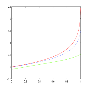
Figure 1: Graphs of the r.h.s. of eq. (81) as a function of $\alpha$. Here, $\sigma^{2}=1/2$, $E_{s}=q=0$ (hence $\tilde{\alpha}_{\mbox{\tiny c}}=1$) and the SNR takes the values: $E_{x}/N_{0}=0.001$ (red), $E_{x}/N_{0}=0.01$ (blue), and $E_{x}/N_{0}=0.1$ (green).

Iterated LPCB

Let $\alpha$ be given and let $\beta_{1},\beta_{2},\ldots,\beta_{k}$ be positive numbers such that $\sum_{i=1}^{k}\beta_{i}<\alpha$. Let $P_{1}$, $P_{2},\ldots,P_{k}$ be a corresponding a sequence of probability measures with $P_{1}\equiv P$ and $P_{k}\equiv Q$, and let $\mbox{\boldmath$E$}_{i}$ denote the expectation operator w.r.t. $P_{i}$, $i=1,2,\ldots,k$. Now consider the following chain of inequalities:

$$\Lambda_{\mbox{\tiny B}}(\hat{\theta},\alpha) \geq \frac{\alpha}{\alpha-\beta_{1}}\ln\mbox{\boldmath$E$}_{2}e^{(\alpha-\beta_{1})(\hat{\theta}-\theta)^{2}}-\frac{\alpha}{\beta_{1}}D_{\alpha/\beta_{1}}(P_{2}\|P_{1})$$ (85)

$$\geq \frac{\alpha}{\alpha-\beta_{1}}\left[\frac{\alpha-\beta_{1}}{\alpha-\beta_{1}-\beta_{2}}\ln\mbox{\boldmath$E$}_{3}e^{(\alpha-\beta_{1}-\beta_{2})(\hat{\theta}-\theta)^{2}}-\frac{\alpha-\beta_{1}}{\beta_{2}}D_{(\alpha-\beta_{1})/\beta_{2}}(P_{3}\|P_{2})\right]-$$

$$\frac{\alpha}{\beta_{1}}D_{\alpha/\beta_{1}}(P_{2}\|P_{1})$$

$$= \frac{\alpha}{\alpha-\beta_{1}-\beta_{2}}\ln\mbox{\boldmath$E$}_{3}e^{(\alpha-\beta_{1}-\beta_{2})(\hat{\theta}-\theta)^{2}}-\frac{\alpha}{\beta_{2}}D_{(\alpha-\beta_{1})/\beta_{2}}(P_{3}\|P_{2})-$$

$$\frac{\alpha}{\beta_{1}}D_{\alpha/\beta_{1}}(P_{2}\|P_{1})$$

$$\geq \frac{\alpha}{\alpha-\sum_{i=1}^{k}\beta_{i}}\ln\mbox{\boldmath$E$}_{k}\exp\left\{\left(\alpha-\sum_{i=1}^{k}\beta_{i}\right)(\hat{\theta}-\theta)^{2}\right\}-$$

$$\alpha\sum_{i=1}^{k-1}\frac{1}{\beta_{i}}D_{(\alpha-\sum_{j=1}^{i-1}\beta_{j})/\beta_{i}}(P_{i+1}\|P_{i}).$$

We now have the freedom to choose the parameters $k$, $\beta_{1},\ldots,\beta_{k}$ and $P_{2},P_{3},\ldots,P_{k}$. The original inequality we have been using (7) is obtained as a special case where $\beta_{i}\downarrow 0$ for $i=1,2,\ldots,k-2,k$, $\beta_{k-1}\uparrow\alpha$, and $P_{2}=P_{3}=\ldots=P_{k-1}=P$ (one can also choose, of course, $k=2$ and $\beta_{1}\uparrow\alpha$, $\beta_{2}\downarrow 0$). The ordinary (one–step) LPBC bound is obtained by choosing $P_{2}=P_{3}=\ldots=P_{k-1}=Q$, $\beta_{1}=\beta<\alpha$ and $\beta_{2}=\beta_{3}=\ldots=\beta_{k}\downarrow 0$ (one can also choose, of course, $k=2$ and $\beta_{1}=\beta$, $\beta_{2}\to 0$). The iterated LPCB can be useful in situations where it is easier to derive (or to bound) the Rényi divergences via certain intermediate reference models rather than going directly from the underlying model to the ultimate reference model (see, e.g., the last part of Subsection 4.1 in [2]).

4.6 Phase Transitions

In this subsection, unlike all other parts of this paper, our focus is not quite only on lower bounds and their tightness, but rather on another aspect of the risk–sensitive cost function, and this is that in some cases, this cost function may exhibit phases transitions, even in rather seemingly simple and innocent parametric models. We have already seen that in many situations where $\theta$ is unbounded, there might be a critical value of the risk–sensitive factor, $\alpha_{\mbox{\tiny c}}$ beyond which this cost function diverges. This is certainly a very sharp (first–order) phase transition. However, in some cases there might be additional phase transitions, due to possible analogies with certain models in statistical mechanics, and the purpose of this subsection is to demonstrate this fact.

Consider the example where $\Theta\sim\mbox{Unif}[0,1]$, $\mbox{\boldmath$y$}\in\{0,1\}^{n}$ and $P(\mbox{\boldmath$y$}|\theta)$ is the Bernoulli distribution,

$$P(\mbox{\boldmath$y$}|\theta)=\theta^{nq}(1-\theta)^{n(1-q)},$$ (86)

where $nq=\sum_{i=1}^{n}y_{i}$ is the number of ones. We would like to investigate the behavior of the risk–sensitive cost function, and our focus will be on the asymptotic behavior at the exponential scale, where $\alpha$ will be assumed to be growing linearly with $n$, that is, we take $\alpha=a\cdot n$ for some fixed $a>0$. We will study the asymptotic exponent of the optimal estimator as a function of $\theta$ and $a$. The optimal Bayesian performance is given by

$$\min_{\hat{\theta}}\mbox{\boldmath$E$}\exp\left\{\alpha n(\hat{\theta}-\theta)^{2}\right\} = \sum_{\mbox{\boldmath$y$}}P(\mbox{\boldmath$y$})\min_{t}\int_{0}^{1}\exp\left\{\alpha n(t-\theta)^{2}\right\}P(\theta|\mbox{\boldmath$y$})\mbox{d}\theta$$ (87)

$$\stackrel{{\scriptstyle\cdot}}{{=}} \sum_{\mbox{\boldmath$y$}}P(\mbox{\boldmath$y$})\min_{t\in[0,1]}\max_{\theta\in[0,1]}\exp\left\{n[a(t-\theta)^{2}-D(q\|\theta)]\right\}$$ (88)

$$\stackrel{{\scriptstyle\cdot}}{{=}} \exp\left\{n\cdot\max_{q\in[0,1]}\min_{t\in[0,1]}\max_{\theta\in[0,1]}\left[a(t-\theta)^{2}-D(q\|\theta)\right]\right\},$$ (89)

where $\stackrel{{\scriptstyle\cdot}}{{=}}$ denotes equality in the exponential scale, and where $D(q\|\theta)$ designates the binary divergence function,

$$D(q\|\theta)=q\ln\frac{q}{\theta}+(1-q)\ln\frac{1-q}{1-\theta}.$$ (90)

The (asymptotically) optimal estimator is then given by

$$\hat{\theta}=\arg\min_{t\in[0,1]}\max_{\theta\in[0,1]}\left[a(t-\theta)^{2}-D(q\|\theta)\right],$$ (91)

which depends on $y$ solely via $q$. This estimator is depicted in Fig. 2 for $a=10$.

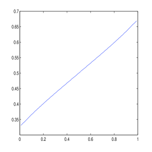
Figure 2: Graph of $\hat{\theta}(q)$. Note that the range of $\hat{\theta}(q)$, which is $[0.331,0.669]$, is much smaller than the domain of $q$, which is $[0,1]$. The estimator avoids extreme values in order not to incur large errors in case the true $\theta$ is in the other extreme. This is due to its risk–sensitive nature.

Obviously,

$$E(a) \stackrel{{\scriptstyle\Delta}}{{=}} \max_{q\in[0,1]}\min_{t\in[0,1]}\max_{\theta\in[0,1]}\left[a(t-\theta)^{2}-D(q\|\theta)\right]$$ (92)

$$\geq \max_{q\in[0,1]}\min_{t\in[0,1]}a(t-q)^{2}$$ (93)

$$\geq 0.$$ (94)

On the other hand, note that by the Pinsker inequality [7], $D(q\|\theta)\geq 2(q-\theta)^{2}$, and so, for $a\in[0,2]$

$$E(a) \leq \max_{q\in[0,1]}\min_{t\in[0,1]}\max_{\theta\in[0,1]}\left[a(t-\theta)^{2}-2(q-\theta)^{2}\right]$$ (95)

$$\leq \max_{q\in[0,1]}\max_{\theta\in[0,1]}\left[a(q-\theta)^{2}-2(q-\theta)^{2}\right]$$ (96)

$$= \max_{q\in[0,1]}\max_{\theta\in[0,1]}(a-2)(q-\theta)^{2}$$ (97)

$$= 0,$$ (98)

and so, it follows that for $a\in[0,2]$, $E(a)=0$ and it is achieved by $\hat{\theta}=q$. The following graph (Fig. 3) displays $E(a)$ and it suggests that $a=2$ is indeed the maximum value of $a$ for which it still vanishes. Thus, we see a phase transition at $a=2$.

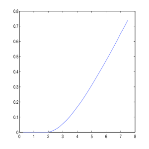
Figure 3: Graph of $E(a)$.

We have seen that the estimator $\hat{\theta}=q$ is asymptotically (exponentially) optimal for every $a\leq 2$. We next analyze the risk–sensitive cost function for this estimator on the exponential scale, and as said, we demonstrate that it also exhibits phase transitions. As already mentioned, it turns out that in some cases, the expression of the exponential moment is analogous to that of a partition function of a certain physical model, in particular, a model of magnetic spins with interactions, which may exhibit phase transitions. To facilitate the presentation of the analogy with statistical mechanics, we now slightly modify our notation. Consider the case where $X$ is a binary vector whose components take on values in ${\cal X}=\{-1,+1\}$, and which is governed by a binary memoryless source $P_{\mu}$ with probabilities $\mbox{Pr}\{X_{i}=+1\}=1-\mbox{Pr}\{X_{i}=-1\}=(1+\mu)/2$, ($\mu$ designating the expected ‘magnetization’ of each binary spin $X_{i}$). The probability of $x$ under $P_{\mu}$ is thus easily shown to be given by

$$P_{\mu}(\mbox{\boldmath$x$})=\left(\frac{1+\mu}{2}\right)^{(n+\sum_{i}x_{i})/2}\cdot\left(\frac{1-\mu}{2}\right)^{(n-\sum_{i}x_{i})/2}=\left(\frac{1-\mu^{2}}{4}\right)^{n/2}\cdot\left(\frac{1+\mu}{1-\mu}\right)^{\sum_{i}x_{i}/2}.$$ (99)

Consider the estimation of the parameter $\mu$ by the ML estimator

$$\hat{\mu}=\frac{1}{n}\sum_{i=1}^{n}x_{i}.$$ (100)

Now,

$$\mbox{\boldmath$E$}_{\mu}\exp\{an(\hat{\mu}-\mu)^{2}\} = \left(\frac{1-\mu^{2}}{4}\right)^{n/2}e^{na\mu^{2}}\sum_{\mbox{\boldmath$x$}}\left(\frac{1+\mu}{1-\mu}\right)^{\sum_{i}x_{i}/2}\exp\left\{\frac{a}{n}\left(\sum_{i}x_{i}\right)^{2}-2a\mu\sum_{i}x_{i}\right\}$$

$$= \left(\frac{1-\mu^{2}}{4}\right)^{n/2}e^{na\mu^{2}}\sum_{\mbox{\boldmath$x$}}\exp\left\{\left(\frac{1}{2}\ln\frac{1+\mu}{1-\mu}-2a\mu\right)\sum_{i}x_{i}+\frac{a}{n}\left(\sum_{i}x_{i}\right)^{2}\right\}.$$

The last summation over $\{\mbox{\boldmath$x$}\}$ is exactly the partition function pertaining to the Curie–Weiss model of spin arrays in statistical mechanics (see, e.g., [23, Subsection 2.5.2]), where the magnetic field is given by

$$B=\frac{1}{2}\ln\frac{1+\mu}{1-\mu}-2a\mu$$ (101)

and the coupling coefficient for every pair of spins is $J=2a$. It is well known that this model exhibits phase transitions pertaining to spontaneous magnetization below a certain critical temperature. In particular, using the method of types [7], this partition function can be asymptotically evaluated as being of the exponential order of

$$\exp\left\{n\cdot\max_{|m|\leq 1}\left[h_{2}\left(\frac{1+m}{2}\right)+Bm+\frac{J}{2}\cdot m^{2}\right]\right\},$$ (102)

where $h_{2}(u)=-u\ln u-(1-u)\ln(1-u)$ is the binary entropy function, which stands for the exponential order of the number of configurations $\{\mbox{\boldmath$x$}\}$ with a given value of $m=\frac{1}{n}\sum_{i}x_{i}=\hat{\mu}$. This expression is clearly dominated by a value of $m$ (the dominant magnetization $m^{*}$) which maximizes the expression in the square brackets, i.e., it solves the equation

$$m=\tanh(Jm+B),$$ (103)

or in our variables,

$$m=\tanh\left(2am+\frac{1}{2}\ln\frac{1+\mu}{1-\mu}-2a\mu\right).$$ (104)

For $a<1/2$, there is only one solution and there is no spontaneous magnetization (paramagnetic phase). For $a>1/2$, however, there are three solutions, and only one of them dominates the partition function, depending on the sign of $B$, or equivalently, on whether $a>a_{0}(\mu)\stackrel{{\scriptstyle\Delta}}{{=}}\frac{1}{4\mu}\ln\frac{1+\mu}{1-\mu}$ or $a<a_{0}(\mu)$ and according to the sign of $\mu$. Accordingly, there are five different phases in the plane spanned by $a$ and $\mu$. The paramagnetic phase $a<1/2$, the phases $\{\mu>0,~{}1/2<a<a_{0}(\mu)\}$ and $\{\mu<0,~{}a>a_{0}(\mu)\}$, where the dominant magnetization $m$ is positive, and the two complementary phases, $\{\mu<0,~{}1/2<a<a_{0}(\mu)\}$ and and $\{\mu>0,~{}a>a_{0}(\mu)\}$, where the dominant magnetization is negative. Thus, there is a multi-critical point where the boundaries of all five phases meet, which is the point $(\mu,a)=(0,1/2)$. The phase diagram is depicted in Fig. 4.

Figure 4: Phase diagram in the plane of $(\mu,\alpha)$.

This analysis can easily be extended to the case of a general parametric family of discrete memoryless source (DMSs), $\{P(\cdot|\theta),~{}\theta\in{\cal A}\}$, where $\theta$ is a parameter vector, and one may replace the square error function by a general loss function $L(\theta,\hat{\theta})$. The class $\{P(\cdot|\theta),~{}\theta\in{\cal A}\}$ may not necessarily span the entire simplex of DMSs of the given alphabet size.

5 The Non–Bayesian Regime

Many of the ideas raised in the previous section may have analogues in the non–Bayesian regime, but we will not derive all of those analogous derivations herein. We will touch only a few important points in this short section.

5.1 The Linear Signal Model

Consider again the signal model,

$$y(t)=x(t,\theta)+n(t),~{}~{}~{}~{}0\leq t\leq T$$ (105)

where $n(t)$ is Gaussian white noise with two–sided spectral density $N_{0}/2$, as before. Consider, for example the case, $x(t,\theta)=\theta\cdot s(t)$, where $\{s(t)\}$ has energy $E_{s}$. Then, if we take $L_{\mbox{\tiny NB}}(\tilde{\theta})$ to be the Cramér–Rao bound, then it is given by $\frac{N_{0}}{2E_{s}}$ independent of $\tilde{\theta}$, and so, according to part 2 of Theorem 1, for any unbiased estimator,

$$\Lambda_{\mbox{\tiny NB}}(\hat{\theta},\theta,\alpha) \geq \sup_{\tilde{\theta}}\left\{\frac{\alpha N_{0}}{2E_{s}}+\left(\alpha-\frac{E_{s}}{N_{0}}\right)(\tilde{\theta}-\theta)^{2}\right\}$$ (106)

$$= \left\{\begin{array}[]{cc}\frac{\alpha N_{0}}{2E_{s}}&\alpha\leq\frac{E_{s}}{N_{0}}\\ \infty&\alpha>\frac{E_{s}}{N_{0}}\end{array}\right.$$ (109)

namely, $\alpha_{\mbox{\tiny c}}\leq E_{s}/N_{0}$. This means that no unbiased estimator has an estimation error $\epsilon$ with a tail that decays faster than $e^{-\epsilon^{2}E_{s}/N_{0}}$. For the maximum likelihood (ML) estimator,

$$\hat{\theta}_{\mbox{\tiny ML}}=\frac{1}{E_{s}}\int_{0}^{T}y(t)s(t)\mbox{d}t=\theta+\frac{1}{E_{s}}\int_{0}^{T}n(t)s(t)\mbox{d}t$$ (110)

and so, the estimation error

$$\epsilon=\hat{\theta}-\theta=\frac{1}{E_{s}}\int_{0}^{T}n(t)s(t)\mbox{d}t$$ (111)

is Gaussian, zero–mean, with variance $\frac{N_{0}}{2E_{s}}$, which attains the upper bound on $\alpha_{\mbox{\tiny c}}$. This means that $E_{s}/N_{0}$ is the exact value of $\alpha_{\mbox{\tiny c}}$ and not merely an upper bound. While in the Bayesian regime, we have for a similar model, $\alpha_{\mbox{\tiny c}}=\frac{1}{2\sigma^{2}}+\frac{E_{s}}{N_{0}}$, here we do not have the contribution of the prior, and the remaining term is just $\frac{E_{s}}{N_{0}}$. It is interesting to note that we obtained a tight result on $\alpha_{\mbox{\tiny c}}$, attained by the ML estimator, even though the bound on $\Lambda_{\mbox{\tiny NB}}(\theta)$ is not attained by the ML estimator, as

$$\Lambda_{\mbox{\tiny NB}}(\hat{\theta}_{\mbox{\tiny ML}},\theta,\alpha)=-\frac{1}{2}\ln\left(1-\frac{\alpha N_{0}}{E_{s}}\right).$$ (112)

The ML estimator achieves, however, the bound asymptotically when $\alpha N_{0}/E_{s}$ is very small, which means, either very small $\alpha$ or very large signal–to–noise ratio, or both.

5.2 The Vector Linear Signal Model

The above derivation extends to the vector case quite easily. Let $x(t,\theta)=\sum_{i=1}^{k}\theta_{i}s_{i}(t)$, where $\{s_{i}(t)\}$ all have the same energy, $E_{s}$ and let $\Gamma$ be the $k\times k$ matrix of correlations with entries given by

$$\gamma_{ij}=\frac{1}{E_{s}}\int_{0}^{T}s_{i}(t)s_{j}(t)\mbox{d}t.$$ (113)

In this case, $D(\tilde{\theta}\|\theta)=(\tilde{\theta}-\theta)^{T}\Gamma(\tilde{\theta}-\theta)$, the Cramér–Rao lower bound is $N_{0}\Gamma^{-1}/2E_{s}$, and so, we get

$$\ln\mbox{\boldmath$E$}_{\theta}\exp\left\{[\alpha^{T}(\hat{\theta}-\theta)]^{2}\right\} \geq \frac{N_{0}\alpha^{T}\Gamma^{-1}\alpha}{2E_{s}}+\sup_{\tilde{\theta}}(\tilde{\theta}-\theta)^{T}\left(\alpha\alpha^{T}-\frac{E_{s}}{N_{0}}\Gamma\right)(\tilde{\theta}-\theta)$$ (114)

$$= \left\{\begin{array}[]{cc}\frac{N_{0}\alpha^{T}\Gamma^{-1}\alpha}{2E_{s}}&\alpha\alpha^{T}\prec\frac{E_{s}}{N_{0}}\Gamma\\ \infty&\mbox{elsewhere}\end{array}\right.$$ (117)

where the notation $A\prec B$, for two $k\times k$ matrices $A$ and $B$, means that $B-A$ is a non-negative definite matrix. The condition $\alpha\alpha^{T}\prec\frac{E_{s}}{N_{0}}\Gamma$ is equivalent to $\alpha^{T}\Gamma^{-1}\alpha<E_{s}/N_{0}$. Here, the estimation error of the ML estimator of $\theta$ is a zero mean Gaussian vector with covariance matrix given by $\frac{N_{0}}{2E_{s}}\Gamma^{-1}$, and so the exponential moment performance of this estimator is given by

$$\Lambda_{\mbox{\tiny NB}}(\hat{\theta}_{\mbox{\tiny ML}},\theta,\alpha)=-\frac{1}{2}\ln\bigg{|}I-\frac{N_{0}}{E_{s}}\alpha\alpha^{T}\Gamma^{-1}\bigg{|}=-\frac{1}{2}\ln\left(1-\frac{N_{0}}{E_{s}}\alpha^{T}\Gamma^{-1}\alpha\right)$$ (118)

which is larger than the lower bound but is asymptotically the same when $\frac{N_{0}}{E_{s}}\alpha^{T}\Gamma^{-1}\alpha\ll 1$. Here $\alpha_{\mbox{\tiny c}}$ is extended from a single point, in the scalar parameter case, to the contour of a $k$–dimensional ellipsoid defined by $\alpha_{\mbox{\tiny c}}^{T}\Gamma^{-1}\alpha_{\mbox{\tiny c}}=E_{s}/N_{0}$, and so, the ML estimator has an optimal tail (in all directions) in this sense.

5.3 The Non–linear Signal Model

Consider next the model (105), where the energy $E_{x}=\int_{0}^{T}x^{2}(t,\theta)\mbox{d}t$ is independent of $\theta$. We will also denote

$$\rho(\theta,\tilde{\theta})=\frac{\int_{0}^{T}x(t,\theta)x(t,\tilde{\theta})\mbox{d}t}{E}.$$ (119)

In this case, the lower bound becomes

$$\Lambda_{\mbox{\tiny NB}}(\hat{\theta}_{\mbox{\tiny ML}},\theta,\alpha)\geq\sup_{\tilde{\theta}}\left[\alpha L_{\mbox{\tiny NB}}(\tilde{\theta})+\alpha(\theta-\tilde{\theta})^{2}-\frac{2E[1-\rho(\theta,\tilde{\theta})]}{N_{0}}\right].$$ (120)

If $L_{\mbox{\tiny NB}}(\tilde{\theta})$ is independent of $\tilde{\theta}$ (which is nearly the case with the Cramér–Rao lower bound in delay, phase and frequency estimation), and if the range ${\cal A}$ of $\theta$ is unlimited, then $\tilde{\theta}$ can be chosen such that the second term is arbitrarily large (whereas the third term is bounded since $|\rho(\theta,\tilde{\theta})|\leq 1$), and so, the lower bound is infinite for every $\alpha>0$, namely, $\alpha_{\mbox{\tiny c}}=0$. In other words, in this case, no unbiased estimator (if at all existent) has a Gaussian tail however slow. If the range of $\theta$ is limited, then, of course, the supermum is finite and it depends on the exact form of $\rho(\cdot,\cdot)$. The same conclusion applies whenever the energy of $x(t,\theta)$ grows slower than quadratically with $\theta$. The conclusion that $\alpha_{\mbox{\tiny c}}=0$ is not surprising in view of the fact that for the same signal model, we obtained $\alpha_{\mbox{\tiny c}}=\frac{1}{2\sigma^{2}}$ in the Gaussian prior case. In the Bayesian case, $\alpha_{\mbox{\tiny c}}$ was positive due to the prior only, and now the prior does not exist anyway, so that $\alpha_{\mbox{\tiny c}}$ vanishes.

References

- [1] R. Atar, K. Chowdhary, and P. Dupuis, “Robust bounds on risk–sensitive functionals via Rényi divergence,” SIAM J. Uncertainty Quant., vol. 3, pp. 18–33, 2015.
- [2] R. Atar and N. Merhav, “Information–theoretic applications of the log–probability comparison bound,” IEEE Trans. Inform. Theory, vol. 61, no. 10, pp. 5366–5386, October 2015.
- [3] R. N. Banavar and J. L. Speyer, “Properties of risk–sensitive filters/estimators,” IEE Proc. Control Theory and Appl., vol. 145, no. 1, January 1998.
- [4] A. Bhattacharyya, “On some analogues of the amount of information and their use in statistical estimation,” Sankhya Indian Journal of Statistics, vol. 8, pp. 1–14, 201–218, 315–328, 1946.
- [5] E. W. Barankin, “Locally best unbiased estimators,” Ann. Math. Statist., vol. 20, pp. 477–501, 1949.
- [6] D. G. Chapman and H. Robbins, “Minimum variance estimation without regularity assumption,” Ann. Math. Statist., vol. 22, pp. 581–586, 1951.
- [7] I. Csiszár and J. Körner, Information Theory: Coding Theorems for Discrete Memoryless Systems, Academic Press, New York, 1981.
- [8] P. Dai Pra, L. Meheghini, and W. J. Runggaldier, “Connections between stochastic control and dynamic games,” Mathematics of Control, Signals and Systems, vol. 9, pp. 303–326, 1996.
- [9] A. Dembo and O. Zeitouni, Large DEviations and Applications, Jones and Bartlett Publishers, London 1993.
- [10] G. B. Di Masi and L. Stettner, “Risk–sensitive control of discrete–time Markov processes with infinite horizon,” SIAM Journal on Control and Optimization, vol. 38, no. 1, pp. 61–78, 1999.
- [11] P. Dupuis and R. S. Ellis, A Weak Convergence Approach to the Theory of Large Deviations, John Wiley & Sons, 1997.
- [12] P. Dupuis, M. R. James, and I. Petersen, “Robust properties of risk–sensitive control,” Mathematics of Control, Signals and Systems, vol. 13, pp. 318–322, 2000.
- [13] W. H. Fleming and D. Hernández–Hernández, “Risk–sensitive control of finite state machines on an infinite horizon I,” SIAM Journal on Control and Optimization, vol. 35, no. 5, pp. 1790–1810, 1997.
- [14] J. Ford, “Risk–sensitive filtering and parameter estimation,” DSTO-TR-0764, published by DSTO Aeronautical and Maritime Research Laboratory, Melbourn, Victoria, Australia, 1999.
- [15] D. A. Fraser and L. Guttman, “Bhattacharyya bound without regularity assumptions,” Ann. Math. Statist., vol. 23, pp. 629–632, 1952.
- [16] R. G. Gallager, Information Theory and Reliable Communication, John Wiley & Sons, New York, 1968.
- [17] Z. Hongguo and C. Peng, “Risk–sensitive fixed–point smoothing estimation for linear discrete–time systems with multiple output delays,” J. Syst. Sci. Complex, vol. 26, pp. 137–150, 2013.
- [18] R. Howard and J. Matheson, “Risk–sensitive Markov decision processes,” Management Science, vol. 18, pp. 356–369, 1972.
- [19] M. R. James, J. S. Baras, and R. J. Elliott, “Risk–sensitive control and dynamic games for partially observed discrete–time nonlinear systems,” IEEE Trans. on Automatic Control, vol. 39, no. 4, pp. 780–792, April 1994.
- [20] J. Keifer, “On minimum variance estimation,” Ann. Math. Statist., vol. 23, pp. 627–629, 1952.
- [21] N. Merhav, “Statistical physics and information theory,” (invited paper) Foundations and Trends in Communications and Information Theory, vol. 6, nos. 1–2, pp. 1–212, 2009.
- [22] N. Merhav, “On optimum strategies for minimizing exponential moments of a loss function,” Communications in Information and Systems, vol. 11, no. 4, pp. 343–368, 2011.
- [23] M. Mézard and A. Montanari, Information, Physics and Computation, Oxford University Press, 2009.
- [24] J. B. Moore, R. J. Elliott, and S. Dey, “Risk–sensitive generalizations of minimum variance estimation and control,” Journal of Mathematical Systems, Estimation and Control, vol. 7, no. 1, pp. 1–15, 1997.
- [25] K. Rajendra Prasad, M. Srinivasan, and T. Satya Savithri, “Robust fading channel estimation under parameter and process noise uncertainty with risk sensitive filter and its comparison with CRLB,” WSEAS Transactions on Communications, vol. 13, pp. 363–371, 2014.
- [26] V. R. Ramezani and S. I. Marcus, “Estimation of hidden Markov models: risk–sensitive filter banks and qualitative analysis of their sample paths,” IEEE Trans. on Automatic Control, vol. 47, no. 12, pp. 1999–2009, December 2002.
- [27] H. L. van Trees, Detection, Estimation, and Modulation Theory, Part I, John Wilty & Sons, New York, 1968.
- [28] Bayesian Bounds for Parametric Estimation and Nonlinear Filtering/Tracking, Edited by H. L. Van Trees and K. L. Bell, John Wiley & Sons, 2007.
- [29] A. J. Weiss, Fundamental Bounds in Parameter Estimation, Ph.D. dissertation, Tel Aviv University, Tel Aviv, Israel, June 1985.
- [30] P. Whittle, “Risk–sensitive linear/quadratic/Gaussian control,” Advances in Applied Probability, vol. 13, pp. 764–777, 1981.
- [31] P. Whittle, “A risk–sensitive maximum principle,” Systems and Control Letters, vol. 15, pp. 183–192, 1990.
- [32] N. Yamamoto and L. Bouten, “Quantum risk–sensitive estimation and robustness,” IEEE Trans. on Automatic Control, vol. 54, no. 1, pp. 92–107, January 2009.