Nonlinear fractional waves at elastic interfaces

Abstract

We derive the nonlinear fractional surface wave equation that governs compression waves at an interface that is coupled to a viscous bulk medium. The fractional character of the differential equation comes from the fact that the effective thickness of the bulk layer that is coupled to the interface is frequency dependent. The nonlinearity arises from the nonlinear dependence of the interface compressibility on the local compression, which is obtained from experimental measurements and reflects a phase transition at the interface. Numerical solutions of our nonlinear fractional theory reproduce several experimental key features of surface waves in phospholipid monolayers at the air-water interface without freely adjustable fitting parameters. In particular, the propagation length of the surface wave abruptly increases at a threshold excitation amplitude. The wave velocity is found to be of the order of 40 cm/s both in experiments and theory and slightly increases as a function of the excitation amplitude. Nonlinear acoustic switching effects in membranes are thus shown to arise purely based on intrinsic membrane properties, namely the presence of compressibility nonlinearities that accompany phase transitions at the interface.

I Introduction

Surface waves are waves that are localized at the interface between two media are at the core of many important everyday life phenomena Rabaud and Moisy (2013); Likar and Razpet (2013); Carcione (2007); Shapiro (2005); Hess (2002); Ben-Menahem and Singh (1981). As a consequence of energy conservation and the interfacial localization, and neglecting dissipative damping effects, the intensity of a surface wave excitation at a planar interface originating from a point source falls of inversely with the distance and not with the inverse squared distance, as for ordinary bulk waves. Consequently, a surface wave emanating from a line excitation travels basically without attenuation in the absence of viscous effects. This demonstrates that surface waves dominate over regular bulk waves at large enough distance and thus explains why they have been amply studied experimentally and theoretically Craik (2004); Thomson (1871); Rayleigh (1885); Airy (1841); Currie et al. (1977); Currie and O’Leary (1978); Borcherdt (2009); Harden et al. (1991); Harden and Pleiner (1994); Lucassen (1968a, b); Lucassen-Reynders and Lucassen (1970); Lucassen and Tempel (1972); Behroozi et al. (2003); Monroy and Langevin (1998). For different systems one finds distinct surface wave types. At the interface between two fluids that have different densities, one finds capillary-gravity waves, the best-known realization of which are deep-water waves at the air-water interface Thomson (1871). Depending on the wave length, these waves are either dominated by gravity or by the interfacial tension. From measurements of the dispersion relation, the functional relationship between wave length and frequency, fluid Behroozi et al. (2010) as well interfacial properties Cinbis and Khuri?Yakub (1992) can be extracted. At the surface of an elastic solid one finds Rayleigh waves, with a dispersion relation that depends on the visco-elastic modulus of the solid Rayleigh (1885); Currie et al. (1977); Currie and O’Leary (1978); Kappler and Netz (2015). Rayleigh and capillary-gravity waves are distinct surface wave types that in fact can, for suitable chosen material parameters, coexist Kappler and Netz (2015). Since they are linear phenomena, i.e. described by a theory that is linear in the surface wave amplitude, they are predicted to travel independently from each other even if they are excited at the same frequency or the same wave length. If the interface in addition to tension exhibits a finite compressibility, a third surface wave type exists, referred to as Lucassen wave Lucassen (1968a, b); Lucassen and Tempel (1972). A well-studied experimental realization is a monolayer of amphiphilic molecules at the air water interfaces Lucassen (1968a, b); Lucassen and Tempel (1972); Harden and Pleiner (1994); Monroy and Langevin (1998). At the experimentally relevant low-frequency range and for realistic values of the interfacial elastic modulus, Lucassen waves exhibit wave lengths in the centimeter range and are thus easily excitable and observable in typical experiments with self-assembled monolayers Lucassen (1968b); Monroy and Langevin (1998).

Wave guiding phenomena in monolayers have recently received focal attention because of the possible connection to nerve-pulse propagation Griesbauer et al. (2012); Shrivastava and Schneider (2014); El Hady and Machta (2015); Heimburg and Jackson (2005); Appali et al. (2012); Rvachev (2010), cell-membrane mediated acoustic cell communication Griesbauer et al. (2009, 2012); Mosgaard et al. (2012); Fichtl et al. (2016) and pressure-pulse-induced regulation of membrane protein function Shrivastava and Schneider (2014); Martinac et al. (1987); Coste et al. (2010). One exciting recent finding was the discovery of nonlinear wave switching phenomena in a simple system of a Dipalmitoylphosphatidylcholine (DPPC) lipid monolayer spread on the air-water interface Shrivastava and Schneider (2014). In the experiments, the wave propagation speed and the wave attenuation were demonstrated to depend in a highly nonlinear fashion on the excitation amplitude, showing almost nothing-or-all behavior: Only above a certain threshold of the excitation amplitude does wave propagation set in, while below that threshold wave transmission is experimentally almost negligible Shrivastava and Schneider (2014). Such a nonlinear switching phenomenon offers a multitude of exciting applications and interpretations, in particular since it is known since a long time that nerve pulse propagation is always accompanied by a mechanical displacement traveling in the axon membrane Kim et al. (2007); El Hady and Machta (2015); Tasaki et al. (1968); Tasaki (1995). In that connection, it should be noted that many membrane proteins are pressure sensitive Martinac et al. (1987); Coste et al. (2010), so the existence of nonlinear acoustic phenomena in membranes constitutes an exquisite opportunity for smart membrane-based regulation and information processing applications Coste et al. (2012); Sukharev and Sachs (2012); Fichtl et al. (2016).

The theoretical description of such nonlinear surface wave phenomena is challenging for several reasons. First of all, the dispersion relation between wave frequency $\omega$ and wave number $k=2\pi/\lambda$ that describes small-amplitude linear surface waves can generally be written as

$$k^{2}\sim\omega^{\alpha},$$ (1)

where we define the dispersion exponent $\alpha$ that allows to classify surface wave equations. For normal compression waves one has $\alpha=2$ and thus the frequency is linearly related to the wave vector. However, for surface waves one typically finds $\alpha\neq 2$. For gravity waves $\alpha=4$, for capillary waves $\alpha=4/3$ and for Lucassen waves one has $\alpha=3/2$ Acheson (1990); Lucassen (1968a).

Nonlinear wave effects (i.e. effects that are nonlinear in the wave amplitude) cannot be simply added on the level of a dispersion relation, since a dispersion relation is obtained by Fourier transforming a linear wave equation and by construction is restricted to the linear regime. Rather, nonlinear effects in the wave amplitude are only captured by a properly derived nonlinear differential equation in terms of the local perturbation field that describes the microscopic wave propagation. This is why in previous theoretical treatments of nonlinear surface waves, the starting point was typically the standard wave equation with $\alpha=2$ and nonlinear effects were introduced phenomenologically Heimburg and Jackson (2005); Villagran Vargas et al. (2011); Mosgaard et al. (2012). It is altogether not clear whether this constitutes an accurate theoretical framework for the description of nonlinear surface compression waves, which Lucassen predicted to have $\alpha=3/2$. On the other hand, hitherto no real-space differential equation for the Lucassen dispersion relation had been derived.

In this article we first derive the linear real-space equation that describes Lucassen surface waves from standard hydrodynamics. We show that these waves are described by a so-called fractional wave equation, which is a differential equation with fractional, i.e. non-integer, time derivative. Although linear fractional wave equations have been amply described in the literature Mainardi (2010); Holm and N sholm (2014); Caputo (1966); Wismer (2006); Jaishankar and McKinley (2012); Wang (2016); Holm et al. (2013), until now no derivation of such an equation based on physical first principles had been available. In a second step, we also include nonlinear effects in the wave amplitude by accounting for the nonlinear interfacial compressibility. The necessary material parameters are taken from our experimental measurements of the interfacial compressibility of DPPC monolayers at the air-water interface. We show that nonlinear effects become dominant for monolayers close to a phase transition, where the 2D elastic modulus (inverse compressibility) becomes small or even vanishes, thus explaining previous experimental observations Shrivastava and Schneider (2014). We solve our nonlinear fractional wave equation numerically and calculate the wave velocity and the compression amplitude as a function of the excitation amplitude. In agreement with experimental observations Shrivastava and Schneider (2014) we find an abrupt decrease of wave damping accompanied by a mild increase in wave velocity above a threshold excitation amplitude. In this comparison, no fitting parameter is used, rather, we extract the nonlinear monolayer compressibility and all other parameters from our experimental measurements.

Our results show that acoustic phenomena at self-assembled phospholipid monolayers are quantitatively described by a nonlinear fractional wave equation derived from physical first principles. Since phospholipids at typical surface pressures are quite close to a phase transition accompanied by a anomalously high interfacial compressibility MacDonald and Simon (1987), nonlinear effects are substantial and lead to a nonlinear dependence of the wave propagation properties on the excitation amplitude. This not only shows that phospholipid layers can guide the propagation of acoustic waves, they can also process these waves in a nonlinear fashion. In this context it is interesting to note that biological membranes are actively maintained at a state close to a membrane phase transition MacDonald and Simon (1987); Hazel (1995); Fichtl et al. (2016), so this nonlinear switching phenomenon could possibly play a crucial role in the communication between pressure-sensitive membrane proteins and other functional units situated in membranes. The resulting acoustic wave speed close to the threshold excitation amplitude is found to be about 40 cm/s both in experiments and theory. Remarkably, this speed is thus in a range comparable to the action potential speed in non-myelinated axons Matsumoto and Tasaki (1977); Ringkamp et al. (2010); Sanders and Whitteridge (1946); Franz and Iggo (1968). The present work should be viewed as a first step in understanding the relation between the acoustic nonlinear membrane wave, treated in this article, and the electrochemically generated action potential, described by the nonlinear Hodgkin-Huxley equations Hodgkin and Huxley (1952).

The structure of this article is as follows: We first sketch the derivation of the dispersion relation for Lucassen waves using linearized theory. We then convert this dispersion relation into a corresponding fractional wave equation. We present a simple physical interpretation of the fractional derivative that appears in the differential equation in terms of the frequency-dependent coupling range of the surface wave excitations to the underlying bulk fluid. It is important to note that the fractional linear wave equation is also systematically derived from interfacial momentum conservation, which is detailed in the Supplemental Information (SI) Kappler et al. . In a second step we include nonlinear effects by accounting for the change of the monolayer compressibility due to the local monolayer density change that accompanies a finite-amplitude surface wave. The resulting nonlinear fractional wave equation is numerically solved in an interfacial geometry that closely mimics the experimental setup used to study surface waves in monolayers at the air-water interface Shrivastava and Schneider (2014). Finally, we compare numerical predictions for the wave velocity and the wave damping with experimental results. This comparison is done without any fitting parameters, as all model parameters are extracted from experiments. The experimental wave speed of about 40 cm/s is very accurately reproduced by the theory. We also reproduce the sudden change of the surface wave propagation properties at a threshold excitation amplitude and thus explain the nonlinear surface wave behavior in terms of the compressibility nonlinearity of a lipid monolayer.

II Derivation of the nonlinear fractional surface wave equation

II.1 Dispersion relation for Lucassen surface waves

We here recapitulate the main steps in the derivation of the Lucassen dispersion relation Lucassen (1968a); Lucassen and Tempel (1972); Harden and Pleiner (1994), complete details can be found in the SI Kappler et al. . We consider a semi-infinite incompressible Newtonian fluid in the half space $z\leq 0$ with shear viscosity $\eta$ and mass density $\rho$, covered by an interface at $z=0$ with two-dimensional excess mass density $\rho_{\mathrm{2D}}$, and which responds elastically under compression, with elastic modulus (inverse compressibility) $K_{\mathrm{2D}}$ Lucassen (1968a, b); Lucassen and Tempel (1972); Harden and Pleiner (1994), see fig. 1.

We start with the linearized incompressible Navier-Stokes equation in the absence of external forces Acheson (1990)

$$\rho\frac{\partial\vec{v}(\vec{r},t)}{\partial t}=-\vec{\nabla}P(\vec{r},t)+\eta\vec{\nabla}^{2}\vec{v}(\vec{r},t)$$ (2)

where $\vec{v}(\vec{r},t)$ is the vectorial velocity field and $P(\vec{r},t)$ is the pressure field. The gradient operator is denoted as $\vec{\nabla}=(\partial/\partial x,\partial/\partial y,\partial/\partial z)$ where the Cartesian coordinates are defined as $\vec{r}=(x,y,z)$. Note that in eq. (2) we have neglected the convective term nonlinear in the velocity field, which is permitted compared to the much stronger nonlinear effects due to surface compression which will be introduced later on, see SI for more details on this Kappler et al. . Relating the velocity field to the time derivative of the displacement field $\vec{u}(\vec{r},t)$ as

$$\vec{v}(\vec{r},t)=\partial\vec{u}(\vec{r},t)/\partial t,$$ (3)

and decomposing the displacement field into the longitudinal and transversal parts according to

$$\vec{u}(\vec{r},t)=\vec{\nabla}\Phi(\vec{r},t)+\vec{\nabla}\times\vec{\Psi}(\vec{r},t),$$ (4)

one finds that the incompressibility condition $\vec{\nabla}\cdot\vec{v}(\vec{r},t)=0$ and the linearized Navier-Stokes eq. (2) can be rewritten as

$$\vec{\nabla}^{2}\Phi(\vec{r},t) =0,$$ (5)

$$\eta\vec{\nabla}^{2}\vec{\Psi}(\vec{r},t) =\rho\partial\vec{\Psi}(\vec{r},t)/\partial t.$$ (6)

Likewise, the pressure profile follows as

$$P(\vec{r},t)=-\rho\partial^{2}\Phi(\vec{r},t)/\partial t^{2}.$$ (7)

To solve eqs. (5), (6) for a wave of frequency $\omega$ and wave number $k$ that is localized in the $xy$-plane and travels along the $x$-direction, we make the harmonic wave ansatz

$$\Phi(\vec{r},t) =\phi e^{z/\lambda_{l}}e^{i(kx-\omega t)},$$ (8)

$$\vec{\Psi}(\vec{r},t) =\hat{e}_{y}\psi e^{z/\lambda_{t}}e^{i(kx-\omega t)},$$ (9)

where the prefactors $\phi$ and $\psi$ are the wave amplitudes and $\hat{e}_{y}$ is the unit vector in the $y$-direction. The decay lengths $\lambda_{l}$ and $\lambda_{t}$ describe the exponential decay of the longitudinal and transversal parts away from the interface in the $z$-direction and follow from the differential eqs. (5) and (6) as

$$\lambda_{l}^{-2} =k^{2},$$ (10)

$$\lambda_{t}^{-2} =k^{2}+\frac{-i\omega\rho}{\eta}.$$ (11)

The ratio of the wave amplitudes $\phi$ and $\psi$ is fixed by the stress continuity boundary condition at the surface, which gives rise to a rather complicated dispersion relation, see SI for a full derivation Kappler et al. . In the long wave length limit, defined by the condition $\rho\omega\gg\eta k^{2}$, the dispersion relation simplifies to

$$k^{2} =\frac{\omega^{2}}{K_{\mathrm{2D}}}\left(\rho_{\mathrm{2D}}+\rho\lambda_{t}\right),$$ (12)

as derived in the SI Kappler et al. . In the same long wave length limit, $\rho\omega\gg\eta k^{2}$, the expression for the transversal decay length eq. (11) simplifies to

$$\lambda_{t}=\sqrt{\frac{\eta}{-i\omega\rho}},$$ (13)

so that we finally obtain, by combining eqs. (12) and (13), the Lucassen dispersion relation

$$k^{2} =\frac{\omega^{2}}{K_{\mathrm{2D}}}\left(\sqrt{\frac{i\rho\eta}{\omega}}+\rho_{\mathrm{2D}}\right).$$ (14)

This expression in fact constitutes a slight generalization of the standard Lucassen dispersion relation Lucassen (1968a) as it additionally contains the interfacial excess mass density $\rho_{\mathrm{2D}}$ Kappler and Netz (2015). This generalized dispersion relation is very useful for our discussion, since it allows to distinguish two important physical limits: In case the coupling to the subphase vanishes, which can be achieved by either sending the bulk viscosity $\eta$ or the bulk density $\rho$ to zero, the first term on the right hand side of eq. (14) vanishes. In this limit we are left with the standard dispersion relation for an elastic wave which involves the elasticity and mass density parameters $K_{\mathrm{2D}}$ and $\rho_{\mathrm{2D}}$ of the interface. On the other hand, if the interfacial excess mass is neglected, i.e. for $\rho_{\mathrm{2D}}=0$, the classical Lucassen dispersion relation is obtained from eq. (14). A simple physical interpretation of eq. (14) will be presented in the next section.

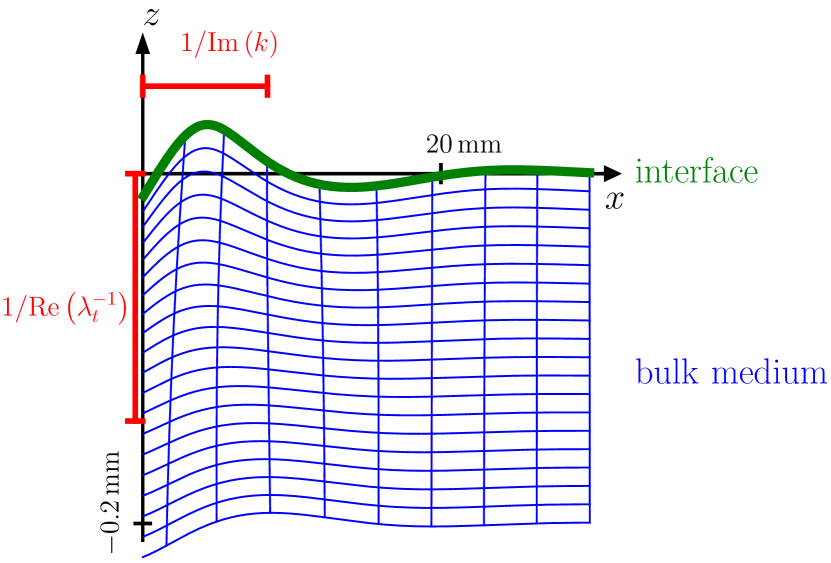
Figure 1: Displacement field of the Lucassen wave. The figure shows the displacement field of a Lucassen wave, given by eqs. (4), (8), (9). The decay lengths in both the $x$- and $z$-directions are shown in red, with $k$, $\lambda_{t}$ given by eqs. (14), (13). For the bulk medium, water is used ($\rho=10^{3}~{}\mathrm{kg/m^{3}}$, $\eta=10^{-3}~{}\mathrm{Pa\cdot s}$); the interface parameters are chosen appropriately for a DPPC monolayer ($K_{\mathrm{2D}}=10~{}\mathrm{mN/m}$, $\rho_{\mathrm{2D}}=10^{-6}~{}\mathrm{kg/m^{2}}$). The shown solution has a frequency $\omega=100~{}\mathrm{s^{-1}}$. Note the anisotropic scaling in $x$- and $z$-direction.

II.2 Fractional linear differential equation for Lucassen surface waves

We now give a simple heuristic derivation of the fractional linear wave equation corresponding to the Lucassen wave. In the SI Kappler et al. , we provide a rigorous derivation based on momentum conservation and utilizing the stress continuity boundary conditions at the interface.

The key observation for arriving at a fractional linear wave equation is that the generalized Lucassen dispersion relation eq. (14) can be rewritten as

$$(ik)^{2}K_{\mathrm{2D}} =(-i\omega)^{2}\rho_{\mathrm{2D}}+(-i\omega)^{3/2}\sqrt{\rho\eta}.$$ (15)

or, using the approximate expression for the longitudinal decay length $\lambda_{t}$, which characterizes the vertical decay of the surface wave Kappler et al. , eq. (13), as

$$(ik)^{2}K_{\mathrm{2D}} =(-i\omega)^{2}(\rho_{\mathrm{2D}}+\lambda_{t}\rho).$$ (16)

The latter equation allows for a simple physical interpretation: The effective area mass density of the interface is given by the sum of the interfacial excess mass density, $\rho_{\mathrm{2D}}$, and the mass density of the bulk fluid layer that via viscosity is coupled to the interface. The area mass density of the coupled bulk fluid layer is $\lambda_{t}\rho$, which is the product of the surface wave decay length $\lambda_{t}$ and the bulk mass density $\rho$. The fractional exponent in eq. (15) emerges because the decay length $\lambda_{t}$ in eq. (13) depends as an inverse square root on the wave frequency $\omega$, reflecting that lower frequencies reach deeper into the fluid bulk medium.

Equation (15) is equivalent to a fractional differential wave equation

$$K_{\mathrm{2D}}\frac{\partial^{2}U(x,t)}{\partial x^{2}}=\rho_{\mathrm{2D}}\frac{\partial^{2}U(x,t)}{\partial t^{2}}+\sqrt{\rho\eta}\frac{\partial^{3/2}U(x,t)}{\partial t^{3/2}},$$ (17)

acting on the displacement of the interface in the $x$-direction, i.e. along the surface, which we define as $U(x,t)=u_{x}(x,z=0,t)$. As in the derivation of eq. (15), the displacement field $U(x,t)$ is independent of $y$, we are thus considering a surface wave front that travels in the $x$-direction and that is translationally invariant in the $y$-direction. The neglect of the interfacial displacement in the $z$-direction is justified in the SI Kappler et al. . The fractional derivative $\partial^{3/2}/\partial t^{3/2}$ on the right hand side is defined in Fourier space, where it amounts to multiplication by $(-i\omega)^{3/2}$ Holm and N sholm (2014); Mainardi (2010). In real space, the fractional derivative in eq. (17) can be formulated using the Caputo formula Caputo (1967); Mainardi (2010)

$$\frac{\partial^{3/2}\,U(x,t)}{\partial t^{3/2}} =\frac{1}{\sqrt{\pi}}\int_{0}^{t}(t-s)^{-1/2}\frac{\partial^{2}\,U(x,s)}{\partial s^{2}}~{}\mathrm{d}s,$$ (18)

which holds for times $t\geq 0$ and where we assume the interface to be in equilibrium at $t=0$ so that both $U(x,t)$ and $\partial U(x,t)/\partial t$ vanish for $t<0$. Thus, eq. (17) is actually an integro-differential equation, which poses a serious challenge for numerical implementations, as we will describe further below.

For a DPPC monolayer on water we have a typical area mass density $\rho_{\mathrm{2D}}=10^{-6}\,\mathrm{kg/m^{2}}$ Griesbauer et al. (2012), the bulk water mass density is $\rho=10^{3}\,\mathrm{kg/m^{3}}$ and the viscosity of water is $\eta=10^{-3}\,\mathrm{Pa\cdot s}$. It follows that for frequencies $\omega\lesssim 10^{7}~{}\mathrm{1/s}$, the effects due to the membrane mass $\rho_{\mathrm{2D}}$ in eq. (15) are negligible compared to the water layer mass. Thus we will for our comparison with experimental data neglect the membrane mass term proportional to $\rho_{\mathrm{2D}}$ in eq. (17) in the following. We note that the resulting fractional linear wave equation has been studied in detail and in fact analytical solutions are well known Schneider and Wyss (1989); Mainardi (2010); Kappler et al. , which we use to test our numerical implementation. For the nonlinear fractional wave equation that we derive in the next section no analytical solutions are known, so that it must be solved numerically.

II.3 Nonlinear compressibility effects

The isothermal elastic modulus $K_{\mathrm{2D}}$ of a lipid monolayer at the air-water interface follows from the surface pressure isotherm $\pi(a)$ as Landau et al. (2008)

$$K_{\mathrm{2D}} =-a\left.\frac{\partial\pi(a)}{\partial a}\right|_{T},$$ (19)

where $a$ is the area per lipid. An experimentally measured isotherm $\pi(a)$ for a DPPC monolayer at room temperature is shown in the inset of fig. 2, the resulting elastic modulus $K_{\mathrm{2D}}$ according to eq. (19) follows by numerical differentiation and is shown in fig. 2 by a solid line. Note that lipid molecules are essentially insoluble in water, so that the number of lipid molecules in the monolayer at the air-water interface stays fixed as the surface pressure is changed, this is why a finite equilibrium compressibility is obtained; such a monolayer is called a Langmuir monolayer. In fig. 2 it is seen that the modulus $K_{\mathrm{2D}}$ depends sensitively on the area per lipid molecule $a$ and exhibits a minimum at an intermediate value of the area. This minimum signals a smeared-out surface phase transition, at which the area per lipid $a$ changes drastically as the surface pressure $\pi$ is varied, as can be clearly seen in the inset of fig. 2. The overall area-dependence of the area modulus $K_{\mathrm{2D}}$ can be well represented by a second order polynomial fit to the experimental data,

$$K_{\mathrm{2D}} =K_{\mathrm{2D}}^{(0)}+K_{\mathrm{2D}}^{(2)}(a-a_{0})^{2}$$ (20)

which is shown as a red broken line in fig. 2. The fit values we extract from our experimental data are $K_{\mathrm{2D}}^{(0)}=2.55$ mN/m, $a_{0}=75.4\,\mathrm{\AA}^{2}$ and $K_{\mathrm{2D}}^{(2)}=0.12$ mN/$\mathrm{\AA}^{2}$.

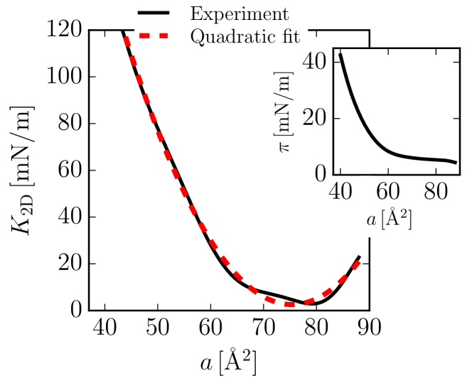
Figure 2: Langmuir isotherm and corresponding isothermal elastic modulus. The inset shows an experimentally measured pressure-area isotherm for a (Langmuir) DPPC monolayer Shrivastava et al. (2015). The main plot shows the corresponding isothermal elastic modulus $K_{\mathrm{2D}}$, as calculated from eq. (19) using the isotherm from the inset. The red dashed line shows a quadratic polynomial fit to the elastic modulus.

The linear wave equation (17) assumes that the local change of the area per lipid during wave propagation is small, so that the elastic modulus $K_{\mathrm{2D}}$ does not change appreciably. This approximation is valid for small wave amplitudes. Obviously, for large wave amplitudes, this assumption breaks down. In fact, for a one-dimensional surface wave characterized by the in-plane displacement field $U(x,t)$, the local time-dependent area per lipid is related to the divergence of the displacement field via Landau et al. (2008)

$$a(x,t) =\bar{a}\left(1+\frac{\partial U(x,t)}{\partial x}\right),$$ (21)

where $\bar{a}$ denotes the equilibrium area per lipid in the absence of the surface wave.

Inserting the expression eq. (21) for the space- and time-dependent area $a(x,t)$ into the parabolic approximation for the elastic modulus eq. (20), we obtain

$$K_{\mathrm{2D}} =K_{\mathrm{2D}}^{(0)}+K_{\mathrm{2D}}^{(2)}\left(\bar{a}+\bar{a}\frac{\partial U(x,t)}{\partial x}-a_{0}\right)^{2},$$ (22)

which constitutes a nonlinear relation between the local elastic modulus $K_{\mathrm{2D}}$ and the interfacial displacement field $U(x,t)$. In deriving this relation, we assume that the experimental isotherm in fig. 2, which is obtained from an equilibrium experiment where the entire monolayer is uniformly compressed at fixed temperature, also describes the local time-dependent elastic response of the monolayer. This assumption requires some discussion: The typical surface wave lengths $\lambda=2\pi/k$ are, in the experimentally relevant frequency range $\omega$ from 1 to $10^{6}$ Hz, in the range of tens of centimeters down to 0.1 mm, as follows directly from the Lucassen dispersion relation eq. (15); they are therefore much larger than the lipid size $\sim\sqrt{a}$ and the locality approximation is not expected to lead to any problems. So we conclude that the expression for the local isothermal elastic modulus eq. (22) is valid to leading order at the length scales of interest.

Combining the displacement-dependent expression for the elastic elastic modulus eq. (22) with the fractional wave equation (17), we finally obtain

$$\left[K_{\mathrm{2D}}^{(0)}+\bar{a}^{2}K_{\mathrm{2D}}^{(2)}\left(1+\frac{\partial U(x,t)}{\partial x}-\frac{a_{0}}{\bar{a}}\right)^{2}\right]\frac{\partial^{2}U(x,t)}{\partial x^{2}}$$

$$=\sqrt{\rho\eta}\frac{\partial^{3/2}U(x,t)}{\partial t^{3/2}},$$ (23)

where, as discussed after eq. (18), we neglect the inertial term proportional to the membrane mass density $\rho_{\mathrm{2D}}$.

This nonlinear fractional wave equation constitutes the central result of our paper, a few comments on the approximations involved and the limits of applicability are in order:

i) We emphasize in our derivation that the displacement $U(x,t)$ is so small that the linearized Navier Stokes equation (2) is valid, while at the same time $U(x,t)$ is large enough so that the assumption of a constant elastic modulus $K_{\mathrm{2D}}$ breaks down. In essence, eq. (II.3) is valid and relevant for an intermediate range of displacement amplitudes. In the SI we show that this assumption is indeed appropriate for the experiments we are comparing with further below Kappler et al. .

ii) Note that when the elastic modulus $K_{\mathrm{2D}}$ depends on the displacement field $U(x,t)$, as demonstrated in eq. (22), it makes a difference whether $K_{\mathrm{2D}}$ appears in front, in between or after the two spatial derivatives in eq. (17). In our nonlinear eq. (II.3), $K_{\mathrm{2D}}$ is positioned in front of the spatial derivatives, so that the derivatives do not act on $K_{\mathrm{2D}}$. This structure of the equation is rigorously derived in the SI Kappler et al. .

iii) The explicit values for the coefficients appearing in the parabolic fit of the experimental elastic modulus in eq. (20) are taken from the equilibrium measurement shown in fig. 2, these values thus correspond to an isothermal measurement at fixed temperature. In the SI, we show that the elastic modulus appropriate for small amplitude Lucassen waves is expected to be somewhat between isothermal and adiabatic, as the time scale of heat transport into the bulk medium is comparable to the oscillation time Kappler et al. . For large wave amplitudes the heat produced or consumed during expansion and compression is therefore not transported into the bulk fluid quickly enough, so that the temperature locally deviates from the environment. For large wave amplitudes the interface deformation is thus expected to become rather adiabatically. The details of this depends on material parameters such as the monolayer heat conductivity and heat capacity, which are not well characterized experimentally. We thus perform our actual numerical calculations with the isothermal values extracted from fig. 2, bearing in mind that this is clearly an approximation.

III Numerical solution

We numerically solve eq. (II.3) in the finite spatial domain $x\in[0,L]$ with the initial condition

$$U(x,t=0) =\frac{\partial U(x,t=0)}{\partial t}=0$$ (24)

for all $x$, corresponding to an initially relaxed and undeformed membrane, and the boundary conditions

$$U(x=0,t) =U_{0}(t)$$ (25)

$$U(L,t) =0.$$ (26)

The function $U_{0}(t)$ in eq. (25) models the mechanical monolayer excitation at the left boundary, $x=0$, which experimentally is produced by a moving piezo-driven blade that is in direct contact with the monolayer at the interface (see ref. Shrivastava and Schneider (2014) for more experimental details). The boundary condition eq. (26) mimics the effects of a bounding wall with vanishing monolayer displacement at a distance $L$ from the excitation source.

We solve the boundary value problem defined by eqs. (II.3-26) by a modification of a general numerical scheme for nonlinear fractional wave equations Li et al. (2011). In the numerics we discretize the equations on 300 grid points and use a system size of $L=3$ cm, which is demonstrated to be large enough so that finite size effects can be neglected Kappler et al. . The accuracy of our numerical scheme is demonstrated by comparison with analytical solutions that are available for the linear fractional wave equation eq. (17). Details of our numerical implementation can be found in the SI Kappler et al. .

For the mechanical boundary excitation $U_{0}(t)$ we use a smoothed pulse function of the form

$$U_{0}(t)=U_{0}^{\mathrm{max}}\cdot\begin{cases}\exp\left[-\left(t-t_{1}\right)^{2}/\tau^{2}\right]\qquad&t<t_{1},\\ 1&t_{1}\leq t\leq t_{2},\\ \exp\left[-\left(t-t_{2}\right)^{2}/\tau^{2}\right]&t_{2}<t,\end{cases}$$ (27)

which mimics the experimental protocol Shrivastava and Schneider (2014). The pulse duration is set by the start and end times, which are fixed at $t_{1}=8.39\,\mathrm{ms}$ and $t_{2}=13.63\,\mathrm{ms}$, the switching time is given by $\tau=2.2\,\mathrm{ms}$, all values are motivated by the experimental boundary conditions, see SI for details Kappler et al. . The amplitude $U_{0}^{\mathrm{max}}$ is the important control parameter that is used to drive the system from the linear into the nonlinear regime. The function $U_{0}(t)$ is shown as dashed black curves in fig. 4(a-c).

For better interpretation of our results, we introduce the negative derivative of the displacement field

$$-U_{x}(x,t)=-\frac{\partial U(x,t)}{\partial x},$$ (28)

which is a dimensionless quantity that is, according to eq. (21), a measure of the relative local lipid area change or compression.

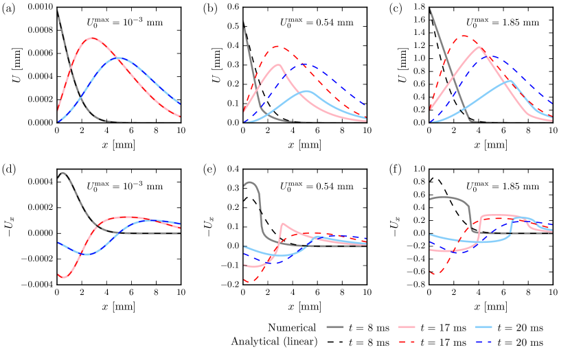
Figure 3: Displacement and compression profiles as a function of position $x$ for a few different fixed times. Results are shown for three different driving amplitudes $U_{0}^{\mathrm{max}}$ as indicated in the figure legends and for a fixed equilibrium area per lipid of $\bar{a}=88.4~{}\mathrm{\AA}^{2}$. Solid lines are obtained by numerical solution of the nonlinear fractional wave equation (II.3). Dashed lines denote analytical solutions of the linear fractional wave equation (17) with $\rho_{\mathrm{2D}}=0$. Compression profiles in the lower row are calculated according to eq. (28).

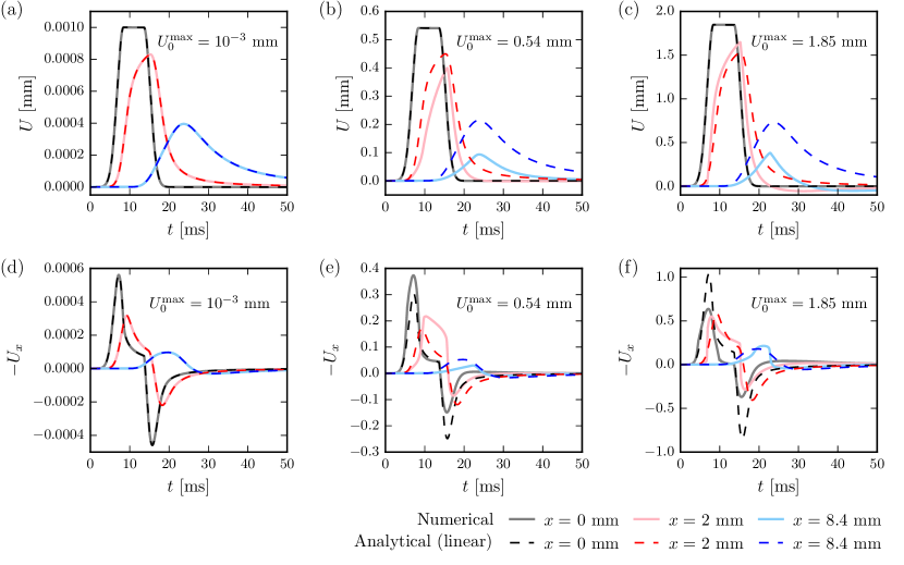
Figure 4: Displacement and compression profiles as a function of time $t$ for a few different fixed separations $x$ from the driven boundary. Results are shown for three different driving amplitudes $U_{0}^{\mathrm{max}}$ as indicated in the figure legends and for a fixed equilibrium area per lipid of $\bar{a}=88.4~{}\mathrm{\AA}^{2}$. Solid lines are obtained by numerical solution of the nonlinear fractional wave equation (II.3). Dashed lines denote analytical solutions of the linear fractional wave equation (17) with $\rho_{\mathrm{2D}}=0$. The dashed black curves for $x=0$ show the driving function $U_{0}(t)$ that is imposed as a boundary condition. Compression profiles in the lower row are calculated according to eq. (28).

We show in fig. 3 numerically calculated solutions of the nonlinear fractional wave equation eq. (II.3) for three different driving amplitudes $U_{0}^{\mathrm{max}}$ as solid colored lines. The equilibrium area per lipid is taken as $\bar{a}=88.4~{}\mathrm{\AA}^{2}$, corresponding to a monolayer that is quite far from the minimum in the area modulus, see fig. 2. The upper row of fig. 3 shows the displacement $U(x,t)$ as a function of position $x$ for a few different fixed times. The lower row shows the corresponding compression profiles $-U_{x}$, defined in eq. (28), which are just the negative spatial derivatives of the displacement profiles in the upper row. The three driving amplitudes $U_{0}^{\mathrm{max}}$ are chosen such as to illustrate the effects of the nonlinear term in eq. (II.3). For the smallest driving amplitude $U_{0}^{\mathrm{max}}=10^{-3}$ mm, the numerically calculated profiles in fig. 3(a) and (d) (solid colored lines) perfectly agree with the analytic solutions of the linearized fractional wave equation (17) (broken colored lines), see SI for details on this comparison Kappler et al. . We thus not only see that the numerical algorithm works, we also find that $U_{0}^{\mathrm{max}}=10^{-3}$ mm is in the linear regime. For the intermediate driving amplitude $U_{0}^{\mathrm{max}}=0.54$ mm in fig. 3(b) and (e) one can discern pronounced deviations between the nonlinear numerical results and the linear predictions, so a sub-millimeter driving amplitude already moves the system deep into the nonlinear regime. For the largest driving amplitude $U_{0}^{\mathrm{max}}=1.85$ mm in fig. 3(c) and (f) we see that the nonlinear equation predicts wave shapes that are completely different from the linear scenario, in particular, the compression profiles in fig. 3(f) exhibit rather sharp fronts.

In fig. 4 we show results for the same parameters, now plotted as a function of time $t$ and for a few different fixed separation $x$ from the source of excitation located at $x=0$. This way of presenting the data is in fact quite close to how nonlinear surface waves are studied experimentally Shrivastava and Schneider (2014). The upper row of fig. 4 again shows the displacement profiles $U(x,t)$ while the lower row shows the corresponding compression profiles $-U_{x}(x,t)$. The black curves for $x=0$ show the excitation pulse that is applied at the boundary $x=0$ which drives the surface wave. Again, we see that for the smallest driving amplitude $U_{0}^{\mathrm{max}}=10^{-3}$ mm in fig. 3(a) and (d) the agreement between the numerical profiles (solid colored lines) and the analytic linear solutions (broken colored lines) is perfect. The wave shape, which at the boundary $x=0$ resembles a pulse with rather sharp flanks, changes into a much smoother function as one moves away from the driven boundary. Distinct deviations between nonlinear and linear predictions occur for larger values of $U_{0}^{\mathrm{max}}$, as shown in the other figures.

Based on $-U_{x}(x,t)$, we consider two observables which are directly measured in our experiments. The first is the maximal local compression at a fixed separation $x$ from the excitation source,

$$-\frac{\Delta a^{\mathrm{min}}(x)}{\bar{a}} =-\min_{t}\left\{\,U_{x}(x,t)\,\right\}.$$ (29)

This maximal compression is in the experiments measured by the locally resolved fluorescence of pressure sensitive dyes that are incorporated into the monolayer Shrivastava and Schneider (2013), as will be further explained below.

The other important observable is the wave speed, defined by

$$c(x)=\frac{x}{t_{\mathrm{min}}(x)-t_{1}+\tau},$$ (30)

where $t_{\mathrm{min}}(x)$ is the time at which the maximal compression with a value of $-\Delta a^{\mathrm{min}}/\bar{a}$ arrives at position $x$, see fig. 5 for a schematic illustration. Note that the denominator in eq. (30) is a measure of the difference of the time at which the boundary excitation $U_{0}(t)$ has risen to $1/e$ of its maximal value, which happens at $t=t_{1}-\tau$, and the time at which the monolayer is maximally compressed at position $x$.

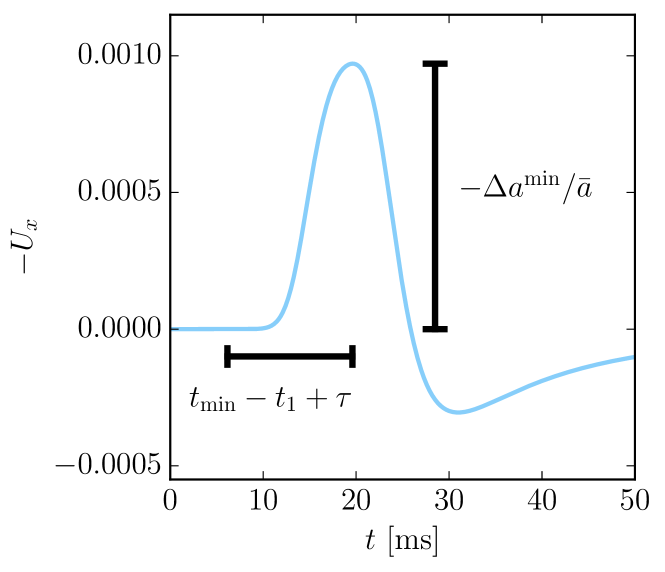
Figure 5: Illustration of the time it takes to observe maximal compression at a fixed position. The blue curve shows the compression field observed at $x=8.4$ mm for a driving amplitude $U_{0}^{\mathrm{max}}=10^{-3}$ mm. The vertical black line indicates the maximal compression $-\Delta a^{\mathrm{min}}/\bar{a}$ at $x=8.4$ mm, i.e. the value of the maximum of the blue curve. The horizontal black line indicates the time difference between the boundary condition rising to $1/e$ of its maximal value, which happens at time $t_{1}-\tau\approx 7$ ms, and the time when the maximal compression is observed at $x=8.4$ mm, $t_{\mathrm{min}}\approx 20$ ms. The difference between these times is used to calculate the wave speed in eq. (30).

In fig. 6(b) we show the maximal compression $-\Delta a^{\mathrm{min}}/\bar{a}$ as defined in eq. (29) as a function of the driving amplitude $U_{0}^{\mathrm{max}}$ at a fixed separation $x=8.4$ mm from the driving boundary, which is the same separation as used in the experiments Shrivastava and Schneider (2014). Different colors correspond to different values of the equilibrium area per lipid $\bar{a}$, all employed values of $\bar{a}$ are denoted in fig. 6(a) by spheres with matching colors, superimposed with the quadratic fit for the monolayer elastic modulus $K_{2D}$ used in the calculations. For small excitation amplitudes $U_{0}^{\mathrm{max}}$ linear behavior is obtained and the maximal compression $-\Delta a^{\mathrm{min}}/\bar{a}$, which in fig. 6(b) is divided by the driving amplitude $U_{0}^{\mathrm{max}}$, exhibits a plateau.

As $U_{0}^{\mathrm{max}}$ is increased, nonlinear effects are noticeable, meaning that the ratio $-\Delta a^{\mathrm{min}}/(\bar{a}U_{0}^{\mathrm{max}})$ depends on $U_{0}^{\mathrm{max}}$. This nonlinear behavior depends sensitively on the equilibrium area per lipid $\bar{a}$ and in particular on whether $\bar{a}$ is larger or smaller than $a_{0}\approx 75\,\mathrm{\AA^{2}}$ for which the elastic modulus $K_{\mathrm{2D}}$ is minimal. For $\bar{a}<a_{0}$ nonlinear effects lead to a monotonic increase of $-\Delta a^{\mathrm{min}}/(\bar{a}U_{0}^{\mathrm{max}})$ with rising $U_{0}^{\mathrm{max}}$, see the violet curve for $\bar{a}=70\,\mathrm{\AA^{2}}$ in fig. 6(b). In contrast, for $\bar{a}>a_{0}$, $-\Delta a^{\mathrm{min}}/(\bar{a}U_{0}^{\mathrm{max}})$ first decreases and then shows a sudden jump as $U_{0}^{\mathrm{max}}$ increases, see the red curve for $\bar{a}=90\,\mathrm{\AA^{2}}$ in fig. 6(b). The latter behavior is close to what has been seen experimentally Shrivastava and Schneider (2014).

The dependence of the wave speed $c$ in fig. 6(c) on the excitation amplitude shows an even more pronounced nonlinear behavior. For $\bar{a}<a_{0}$ nonlinear effects lead to a monotonic and smooth increase of the wave speed as a function of the driving amplitude $U_{0}^{\mathrm{max}}$, while for $\bar{a}>a_{0}$ the speed decreases slightly and then abruptly increases at a threshold amplitude of about $U_{0}^{\mathrm{max}}=2$ mm. These excitation amplitudes are easily reached experimentally and thus relevant to the experimentally observed nonlinear effects, as will be discussed later.

The nonlinear monolayer response can be rationalized in the following fashion: For an initial area $\bar{a}=70\mathrm{\AA^{2}}$, in the compressive part of the pulse, i.e. where $-U_{x}>0$, the monolayer is compressed and thus characterized by a smaller local area $a<\bar{a}$. From fig. 6(a) it becomes clear that since $\bar{a}$ is located to the left of the minimum at $a_{0}$, this compression increases the local area modulus. Within the linear Lucassen theory, the characteristic length that characterizes the damping along the wave propagation direction is given by

$$\lambda_{\parallel}=\frac{1}{\mathrm{Im}(k)}\sim\sqrt{K_{\mathrm{2D}}},$$ (31)

while the phase velocity follows as

$$c_{\parallel}=\frac{\omega}{\mathrm{Re}(k)}\sim\omega\sqrt{K_{\mathrm{2D}}},$$ (32)

where we used the result in eq. (14) for the wave number $k(\omega)$. We see that a larger elastic modulus $K_{\mathrm{2D}}$ not only leads to a larger damping length $\lambda_{\parallel}$ but also to a larger phase velocity $c_{\parallel}$. Thus, for $\bar{a}<a_{0}$, nonlinear effects are expected to increase the range and the speed of the surface waves, as indeed seen in fig. 6.

For initial areas $\bar{a}>a_{0}$, on the other hand, a small local compression will decrease $K_{\mathrm{2D}}$ and only beyond a certain threshold driving amplitude be expected to increase $K_{\mathrm{2D}}$. We can thereby explain the non-monotonic behavior of the maximal compression and the wave speed seen in the numerical data in figs. 6(b) and (c) in a quite simple manner. In physical terms, the minimum in range and velocity for $\bar{a}>a_{0}$ occurs when nonlinear compression effects are large enough to locally drive the membrane into the minimum in the area modulus $K_{\mathrm{2D}}$ located at $a_{0}$.

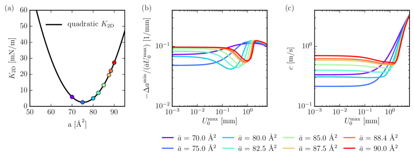
Figure 6: Numerical nonlinear results. (a) Black line: Quadratic fit to the elastic modulus shown in fig. 2. Colored dots: The different initial areas per lipid $\bar{a}$ used for generating subplots (b), (c). (b), (c) Numerical results for the boundary value problem given by eqs. (II.3-26), with the boundary condition given by eq. (27) and the quadratic $K_{\mathrm{2D}}$ shown in subplot (a), for different initial areas per molecule $\bar{a}$. Subplot (b) shows the maximal compression $-\Delta a^{\mathrm{min}}/\bar{a}$ at a distance $x=8.4$ mm from the excitation source, calculated using eq. (29) and divided by $U_{0}^{\mathrm{max}}$. Subplot (c) shows the corresponding wave velocity $c$ according to eq. (30).

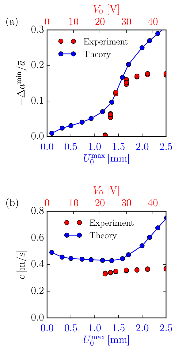
Figure 7: Comparison of numerical and experimental results at a distance $x=8.4$ mm from the excitation source as a function of the excitation amplitude. The numerical data is obtained by solution of the boundary value problem given by eqs. (II.3-26), with the boundary condition given by eq. (27) and the quadratic elastic modulus $K_{\mathrm{2D}}$ shown in fig. 2, and various driving amplitudes $U_{0}^{\mathrm{max}}$. The initial area per lipid $\bar{a}=88.4\,\mathrm{\AA}^{2}$ corresponds to an initial pressure $\pi=4.3\,\mathrm{mN/m}$, c.f. fig. 2. Observables are calculated using eqs. (29), (30), with $x=8.4$ mm. The experimental data is obtained by exciting waves in a DPPC monolayer on a Langmuir trough filled with water using various driving voltages $V_{0}$, and measuring the FRET efficiency of pressure sensitive fluorophores at distance $x=8.4$ mm away from the excitation source Shrivastava and Schneider (2014); Shrivastava et al. (2015). The equilibrium surface pressure of the DPPC monolayer is $\pi=4.3$ mN/m.

IV Comparison with experimental data

Nonlinear surface waves in a DPPC monolayer have been recently discovered experimentally Shrivastava and Schneider (2013, 2014); Shrivastava et al. (2015). In the experimental setup, a DPPC monolayer that contains a small amount of pressure-sensitive fluorophores is spread at the air-water interface. A razor blade is placed on top of the interface so that it touches the monolayer at a line. A piezo element is used to drive the blade laterally and thereby to compress the monolayer at one end. The excitation pulse shape resembles the smoothed rectangular pulse defined in eq. (27). At a fixed separation $x=8.4~{}{\mathrm{mm}}$ from the razor blade a fast camera records the fluorescence resonance energy transfer (FRET) efficiency of the fluorophores as a function of time. Using an independent measurement of the FRET efficiency as a function of the area per lipid for an equilibrium isothermal compression of a DPPC monolayer, the recorded time-dependent FRET efficiency is converted into the time-dependent area per lipid $a(t)$, as described in detail before Shrivastava et al. (2015). Waves are excited using different driving voltage amplitudes $V_{0}$ of the piezo element, for each value of $V_{0}$ the FRET efficiency as a function of time is recorded and converted to yield the compression $\Delta a(t)=a(t)-\bar{a}$. From the maximum of $\Delta a(t)$ the maximal compression $-\Delta a^{\mathrm{min}}$ at a separation $x=8.4\,\mathrm{mm}$ and the time shift $t_{\mathrm{min}}$ at which this maximal compression occurs are calculated Shrivastava et al. (2015). Figure 7(a) shows the experimental results for the relative maximal compression $-\Delta a^{\mathrm{min}}/\bar{a}$ (red spheres) as a function of the piezo driving potential $V_{0}$. The data show a steep increase at a threshold excitation amplitude and level off at a compression of roughly $-\Delta a^{\mathrm{min}}/\bar{a}\approx 0.2$. The wave velocity in fig. 7(b) slightly increases with rising driving voltage and is in the order $c\approx 0.35$ m/s.

To compare with our theoretical results we evaluate eqs. (II.3-26) at an equilibrium lipid area $\bar{a}=88.4~{}\mathrm{\AA^{2}}$, which corresponds to the experimental equilibrium surface pressure $\pi=4.3\,\mathrm{mN/m}$, see fig. 2. For different values of the excitation amplitude $U_{0}^{\mathrm{max}}$ we calculate the maximal compression and the wave velocity $c$ at a separation $x=8.4$ mm using eqs. (29) and (30). Figure 7 shows that our theory (blue data points connected by lines) is in reasonable agreement with the experiments, the only adjustable parameter in the comparison is a rescaling of the driving amplitude $U_{0}^{\mathrm{max}}$, which is necessary since the piezo voltage can not precisely be converted to the oscillation amplitude of the razor blade. The theoretical maximal relative compression $-\Delta a^{\mathrm{min}}/\bar{a}$ shows a quite sharp increase of the relative compression from around $-\Delta a^{\mathrm{min}}/\bar{a}\approx 0.1$ to $-\Delta a^{\mathrm{min}}/\bar{a}\approx 0.2$, while the experimental data seem to increase from $-\Delta a^{\mathrm{min}}/\bar{a}\approx 0$ to $-\Delta a^{\mathrm{min}}/\bar{a}\approx 0.2$. In both theory and experiment, at the threshold driving amplitude a slight increase in the wave velocity is obtained, the value of the wave velocity is quite similar in experiments and theory. This is remarkable, since no freely adjustable parameter is present in the theory.

One possible reason for the deviations between theory and experiments is that our theoretical model employs the isothermal elastic modulus extracted from the equilibrium pressure isotherm shown in fig. 2. This is an approximation, since the temperature is not expected to be strictly constant during the wave propagation, as mentioned before Kappler et al. . Indeed, it is well known that isotherms obtained from compressing a monolayer depend on the compression speed used Klopfer and Vanderlick (1996) and that the slowest relaxation modes in a lipid monolayer are on time scales comparable to those of the wave oscillation time Holzwarth (1989), so that the elastic modulus relevant for the non-equilibrium phenomenon of a propagating surface wave might differ significantly from the isothermal elastic modulus characterizing the quasi-static monolayer compression. In fact, our theory might be used to shed light on the transition of monolayer elasticity from the isothermal to the adiabatic regime, as will be explained below.

V Conclusions

We have derived a fractional wave equation for a compressible surface wave on a viscous liquid from classical hydrodynamic equations. This fractional wave equation has a simple physical interpretation in terms of the frequency-dependent penetration depth of the surface wave into the liquid subphase. Our derivation complements previous approaches where fractional wave equations were obtained by invoking response functions with fractional exponents Caputo (1966); Wismer (2006); Jaishankar and McKinley (2012); Wang (2016); Holm et al. (2013), and constitutes the first derivation of a fractional wave equation from first physical principles. Therefore, on a fundamental level, our theory sheds light on how fractional wave behavior emerges from the viscous coupling of an interface to the embedding bulk medium.

For the explicit system of a monolayer at the air-water interface, nonlinear behavior emerges naturally since large monolayer compression changes the local monolayer compressibility. Our theory describes the experimentally observed nonlinear acoustic wave propagation in a DPPC monolayer without adjustable fit parameters. In particular, the “all-or-nothing” response for the maximal compression of a monolayer as a function of the driving amplitude is reproduced and explained by the fact that the acoustic wave locally drives the monolayer through a phase transition.

Our theory reveals the origin of nonlinear behavior of pressure waves in compressible monolayers, which are fundamentally different from the nonlinear mechanism for action potential propagation. The connection between these two phenomena, which experimentally are always measured together, have fascinated researchers from different disciplines for a long time Tasaki et al. (1989); Heimburg and Jackson (2005); Griesbauer et al. (2012); Shrivastava and Schneider (2014); El Hady and Machta (2015).

Our theory might also be used to extract non-equilibrium mechanical properties of biomembranes: Experimental monolayer compressibilities depend on the compression speed employed in the measurement Klopfer and Vanderlick (1996), consequently the elastic modulus that enters the Lucassen wave theory is neither strictly isothermal nor adiabatic Kappler et al. . Our theory could via inversion be used to extract the elastic modulus from experimentally measured surface wave velocities and thereby help to bridge the gap from isothermal membrane properties to adiabatic membrane properties, which is relevant for membrane kinetics.

References

- Rabaud and Moisy (2013) M. Rabaud and F. Moisy, Physical Review Letters 110 (2013), 10.1103/PhysRevLett.110.214503.
- Likar and Razpet (2013) A. Likar and N. Razpet, American Journal of Physics 81, 245 (2013).
- Carcione (2007) J. J. M. Carcione, Wave Fields in Real Media: Wave Propagation in Anisotropic, Anelastic, Porous and Electromagnetic Media, Handbook of Geophysical Exploration: Seismic Exploration (Elsevier Science, 2007).
- Shapiro (2005) N. M. Shapiro, Science 307, 1615 (2005).
- Hess (2002) P. Hess, Physics Today 55, 42 (2002).
- Ben-Menahem and Singh (1981) A. Ben-Menahem and S. J. Singh, Seismic Waves and Sources (Springer New York, New York, NY, 1981) oCLC: 852790405.
- Craik (2004) A. D. D. Craik, Annual Review of Fluid Mechanics 36, 1 (2004).
- Thomson (1871) W. Thomson, Nature 5, 1 (1871).
- Rayleigh (1885) L. Rayleigh, Proceedings of the London Mathematical Society s1-17, 4 (1885).
- Airy (1841) G. B. Airy, Encyclopedia Metropolitana 3 (1841).
- Currie et al. (1977) P. K. Currie, M. A. Hayes, and P. O’Leary, Q. Appl. Math. 35, 35 (1977).
- Currie and O’Leary (1978) P. K. Currie and P. O’Leary, Q. Appl. Math. 36, 445 (1978).
- Borcherdt (2009) R. D. Borcherdt, Viscoelastic Waves Layered Media (Cambridge University Press, 2009).
- Harden et al. (1991) J. L. Harden, H. Pleiner, and P. A. Pincus, The Journal of Chemical Physics 94, 5208 (1991).
- Harden and Pleiner (1994) J. Harden and H. Pleiner, Physical Review E 49, 1411 (1994).
- Lucassen (1968a) J. Lucassen, Trans. Faraday Soc. 64, 2230 (1968a).
- Lucassen (1968b) J. Lucassen, Trans. Faraday Soc. 64, 2221 (1968b).
- Lucassen-Reynders and Lucassen (1970) E. Lucassen-Reynders and J. Lucassen, Advances in Colloid and Interface Science 2, 347 (1970).
- Lucassen and Tempel (1972) J. Lucassen and M. V. D. Tempel, Journal of Colloid and Interface Science 41, 491 (1972).
- Behroozi et al. (2003) F. Behroozi, B. Lambert, and B. Buhrow, ISA Transactions 42, 3 (2003).
- Monroy and Langevin (1998) F. Monroy and D. Langevin, Physical Review Letters 81, 3167 (1998).
- Behroozi et al. (2010) F. Behroozi, J. Smith, and W. Even, American Journal of Physics 78, 1165 (2010).
- Cinbis and Khuri?Yakub (1992) C. Cinbis and B. T. Khuri?Yakub, Review of Scientific Instruments 63, 2048 (1992).
- Kappler and Netz (2015) J. Kappler and R. R. Netz, EPL (Europhysics Letters) 112, 19002 (2015).
- Griesbauer et al. (2012) J. Griesbauer, S. B ssinger, A. Wixforth, and M. F. Schneider, Phys. Rev. Lett. 108, 198103 (2012).
- Shrivastava and Schneider (2014) S. Shrivastava and M. F. Schneider, Journal of The Royal Society Interface 11, 20140098 (2014).
- El Hady and Machta (2015) A. El Hady and B. B. Machta, Nature Communications 6, 6697 (2015).
- Heimburg and Jackson (2005) T. Heimburg and A. D. Jackson, Proceedings of the National Academy of Sciences 102, 9790 (2005).
- Appali et al. (2012) R. Appali, U. van Rienen, and T. Heimburg, in Advances in Planar Lipid Bilayers and Liposomes, Vol. 16 (Elsevier, 2012) pp. 275–299.
- Rvachev (2010) M. M. Rvachev, Biophysical Reviews and Letters 05, 73 (2010).
- Griesbauer et al. (2009) J. Griesbauer, A. Wixforth, and M. F. Schneider, Biophysical journal 97, 2710 (2009).
- Mosgaard et al. (2012) L. D. Mosgaard, A. D. Jackson, and T. Heimburg, in Advances in Planar Lipid Bilayers and Liposomes, Vol. 16 (Elsevier, 2012) pp. 51–74.
- Fichtl et al. (2016) B. Fichtl, S. Shrivastava, and M. F. Schneider, Scientific Reports 6, 22874 (2016).
- Martinac et al. (1987) B. Martinac, M. Buechner, A. H. Delcour, J. Adler, and C. Kung, Proceedings of the National Academy of Sciences 84, 2297 (1987).
- Coste et al. (2010) B. Coste, J. Mathur, M. Schmidt, T. J. Earley, S. Ranade, M. J. Petrus, A. E. Dubin, and A. Patapoutian, Science 330, 55 (2010).
- Kim et al. (2007) G. H. Kim, P. Kosterin, A. L. Obaid, and B. M. Salzberg, Biophysical journal 92, 3122 (2007).
- Tasaki et al. (1968) I. Tasaki, A. Watanabe, R. Sandlin, and L. Carnay, Proceedings of the National Academy of Sciences of the United States of America 61, 883 (1968).
- Tasaki (1995) I. Tasaki, Biochemical and biophysical research communications 215, 654 (1995).
- Coste et al. (2012) B. Coste, B. Xiao, J. S. Santos, R. Syeda, J. Grandl, K. S. Spencer, S. E. Kim, M. Schmidt, J. Mathur, A. E. Dubin, M. Montal, and A. Patapoutian, Nature 483, 176 (2012).
- Sukharev and Sachs (2012) S. Sukharev and F. Sachs, Journal of Cell Science 125, 3075 (2012).
- Acheson (1990) D. J. Acheson, Elementary fluid dynamics, Oxford applied mathematics and computing science series (Clarendon Press ; Oxford University Press, Oxford : New York, 1990).
- Villagran Vargas et al. (2011) E. Villagran Vargas, A. Ludu, R. Hustert, P. Gumrich, A. D. Jackson, and T. Heimburg, Biophysical Chemistry 153, 159 (2011).
- Mainardi (2010) F. Mainardi, Fractional Calculus and Waves in Linear Viscoelasticity: An Introduction to Mathematical Models (IMPERIAL COLLEGE PRESS, 2010).
- Holm and N sholm (2014) S. Holm and S. P. N sholm, Ultrasound in Medicine & Biology 40, 695 (2014).
- Caputo (1966) M. Caputo, Annals of Geophysics 19, 383 (1966).
- Wismer (2006) M. G. Wismer, The Journal of the Acoustical Society of America 120, 3493 (2006).
- Jaishankar and McKinley (2012) A. Jaishankar and G. H. McKinley, Proceedings of the Royal Society A: Mathematical, Physical and Engineering Sciences 469, 20120284 (2012).
- Wang (2016) Y. Wang, Geophysical Journal International 204, 1216 (2016).
- Holm et al. (2013) S. Holm, S. P. N sholm, F. Prieur, and R. Sinkus, Computers & Mathematics with Applications 66, 621 (2013).
- MacDonald and Simon (1987) R. C. MacDonald and S. A. Simon, Proceedings of the National Academy of Sciences 84, 4089 (1987).
- Hazel (1995) J. R. Hazel, Annual Review of Physiology 57, 19 (1995).
- Matsumoto and Tasaki (1977) G. Matsumoto and I. Tasaki, Biophysical Journal 20, 1 (1977).
- Ringkamp et al. (2010) M. Ringkamp, L. M. Johanek, J. Borzan, T. V. Hartke, G. Wu, E. M. Pogatzki-Zahn, J. N. Campbell, B. Shim, R. J. Schepers, and R. A. Meyer, PLoS ONE 5, e9076 (2010).
- Sanders and Whitteridge (1946) F. K. Sanders and D. Whitteridge, The Journal of Physiology 105, 152 (1946).
- Franz and Iggo (1968) D. N. Franz and A. Iggo, The Journal of Physiology 199, 319 (1968).
- Hodgkin and Huxley (1952) A. L. Hodgkin and A. F. Huxley, The Journal of Physiology 117, 500 (1952).
- (57) J. Kappler, S. Shrivastava, M. F. Schneider, and R. R. Netz, “See supplemental information for detailed derivations and the numerical algorithm,” .
- Caputo (1967) M. Caputo, Geophysical Journal International 13, 529 (1967).
- Schneider and Wyss (1989) W. R. Schneider and W. Wyss, Journal of Mathematical Physics 30, 134 (1989).
- Landau et al. (2008) L. D. Landau, E. M. Lif?ic, and L. D. Landau, Theory of elasticity, 3rd ed., Course of theoretical physics No. Vol. 7 (Elsevier, Amsterdam, 2008) oCLC: 934382464.
- Shrivastava et al. (2015) S. Shrivastava, K. H. Kang, and M. F. Schneider, Physical Review E 91 (2015), 10.1103/PhysRevE.91.012715.
- Li et al. (2011) C. Li, Z. Zhao, and Y. Chen, Computers & Mathematics with Applications 62, 855 (2011).
- Shrivastava and Schneider (2013) S. Shrivastava and M. F. Schneider, PLoS ONE 8, e67524 (2013).
- Klopfer and Vanderlick (1996) K. Klopfer and T. Vanderlick, Journal of Colloid and Interface Science 182, 220 (1996).
- Holzwarth (1989) J. F. Holzwarth, in The Enzyme Catalysis Process, edited by A. Cooper, J. L. Houben, and L. C. Chien (Springer US, Boston, MA, 1989) pp. 383–412.
- Tasaki et al. (1989) I. Tasaki, K. Kusano, and P. Byrne, Biophysical Journal 55, 1033 (1989).