Skyrmion Lattices in Electric Fields

Abstract

This paper studies the influence of electric fields on the skyrmion lattice (SkL) in insulating skyrmion compounds with weak magnetoelectric (ME) coupling. The ME coupling mechanism is an interaction between the external electric field $E$ and local magnetization in the sample. Physically, the $E$-field perturbs the spin modulation wave vectors resulting in the distortion of the SkL and the $E$-field induced shift in energy. Due to the relativistic smallness of ME coupling, the important physics is captured already in the elastic ($\propto$$E$) and inelastic ($\propto$$E^{2}$) responses. In this spirit, the effect of the fourth-order cubic anisotropy responsible for stabilization of the skyrmion phase is taken into account perturbatively. The shift in energy can be either positive or negative, – depending on the direction of electric field, – thus stabilizing or destabilizing the SkL phase. Understanding the $E$-field energetics is important from the viewpoint of creation (writing) and destruction (erasing) of skyrmion arrays over the bulk, which is paramount for developing skyrmion-based logical elements and data storage.

Introduction

Magnetic skyrmions are quasiparticles built from topologically protected vortices of spins in helimagnets. They were theoretically predicted by Bogdanov in 1989 as thermodynamically stable states of chiral magnets,Bogdanov1989 and discovered twenty years after in the form of a hexagonal skyrmion lattice in the helimagnetic conductor MnSi.Binz2006 ; Muhlbauer2009 The magnetic skyrmions gained their name after T. Skyrme, who introduced such field configurations in the context of low-energy physics of mesons and baryons Skyrme1961 to explain the stability of particles through topological protection against continuous field transformations. Currently, skyrmions in chiral magnets are compelling due to their nanoscale size and the mentioned topological protection: They are envisaged as promising information carriers, and the skyrmion racetrack memory was recently proposed, see e.g. Refs. Fert2013 ; Nagaosa2013 ; Racetrack1 ; Racetrack2 ; Racetrack3

As quasiparticles, skyrmions can form a crystalline state, and solid-state concepts, such as symmetry breaking, order parameter, elementary excitations etc., can be applied, therefore opening doors for simple but very efficient theoretical models. The skyrmion crystal was observed both in the reciprocal and real space in the form of a two-dimensional hexagonal lattice, Muhlbauer2009 ; Tonomura2012 as is sketched in Figure 1. The hallmark of the skyrmion lattice (SkL) as seen by SANS (small angle neutron scattering) is the appearance of a six-fold pattern in reciprocal space.Muhlbauer2009 ; Munzer2010 ; Tokunaga2015 ; Adams2012 ; White2014 The thermodynamical stability of skyrmion lattices is improved experimentally by continuous tuning of coupling parameters with hydrostatic pressure Levatic2016 or by perturbing the skyrmion lattice with electric fields. Okamura2016 The interest in the skyrmion lattices and their stability is justified by the solid-state concept that the lattice could be melted into individual skyrmions.

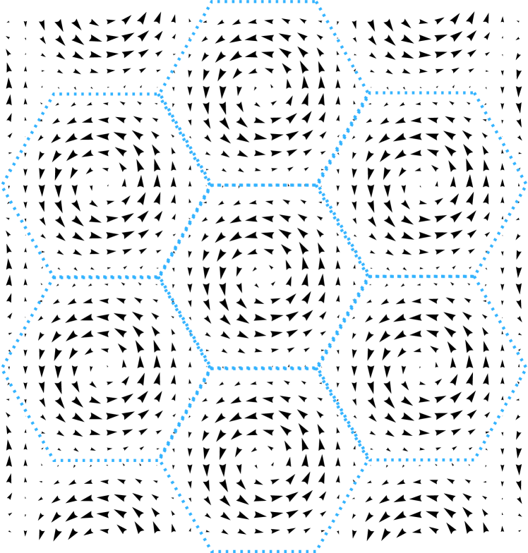
Figure 1: The hexagonal skyrmion lattice (real space), as a schematic projection of spins on the basal plane. The dotted lines (blue) denote the in-plane periodicities of the SkL vector order parameter.

Manipulation and control of skyrmions have become an active topic of skyrmionics. Recent experiments succeeded manipulation of skyrmions with moderate electric fields, electric currents , and thermal gradients. White2012 ; White2014 ; Jonietz2010 ; Yu2012 ; Jiang2015 ; Everschor2012 ; Mochizuki2014 ; Watanabe2016 To avoid the Ohmic heating effects which are undesirable for electronics, the application of moderate electric fields to insulating skyrmion-host compounds (such as ${\text{Cu}_{2}\text{O}\text{Se}\text{O}_{3}}$ Seki2012 ) is potentially more advantageous for the current-driven devices. These observations motivated theoretical proposals for creation (“writing”) skyrmions in insulating helimagnets with the help of external electric field, Mochizuki2015 ; Mochizuki2016 ; Okamura2016 ; Watanabe2016 and subsequent electric-field guiding. Upadhyaya2015 To date, a key experimental challenge in this direction is stabilization and control of the skyrmion lattice by an electric field. Therefore, there is an urge for simple theories of skyrmion lattice response to the E-field. In particular, what is of interest is the shift of skyrmion lattice energy in electric field, with subsequent stabilization of the skyrmion lattice.Okamura2016

In the present paper we discuss the physics of the skyrmion lattice upon application of $E$-field to an insulating skyrmion-host compound, such as ${\text{Cu}_{2}\text{O}\text{Se}\text{O}_{3}}$. In this material, the effect of magnetoelectric coupling arises due to a hybridization mechanism originating from relativistic spin-orbit interaction (see Refs. Seki2012 ; Liu2013 ; Nagaosa2007 ; Belesi2012 ), which gives rise to an electric dipole moment which can be expressed in terms of the local spin variables. The strength of the effect is however relativistically small, which allows us to build an accurate perturbation theory in $E$-fields.

In this paper, we treat the effect of electric field on skyrmion lattices in the two first orders of perturbation theory. The skyrmion lattice in electric fields becomes slightly distorted, and we introduce the elastic and inelastic distortion vectors. The shift of SkL energy comes from expectation values of the electromagnetic coupling and anisotropic contributions.

This paper is organized as follows. In Sec. I, we write down the effective coarse-grained energy functional, and make a rotation of quantization axes, as demanded by the experimental orientation of magnetic field. In Sec. II, we consider the mean-field treatment for the SkL energy density with the magnetic field applied. In Sec. III, we calculate the distortion of the skyrmion lattice by the electric field in an elastic approximation. In Sec. IV, we first calculate the mean-field expectation value of the electromagnetic coupling term, also taking into account the distortion-induced anisotropic contributions. To be consistent in the first two orders of perturbation expansion, we introduce the inelastic distortion vector, and write down all the terms in first and second orders in dimensionless electric field $\ae$. In the concluding section we highlight the main results and discuss the limitations of the model and possible applications.

I Energy density in a coarse-grained model

The Skyrmion Lattice (SkL) is a long-range-order spin configuration which can be visualized as a hexagonal array of vortices (see Fig. 1). Experimentally, the hallmark of the SkL phase is appearance of a six-fold reflection pattern in reciprocal space, as sketched in Fig. 2, each of the wave vectors are rotated by $2\pi/3$ (see e.g. Refs. Muhlbauer2009 ; White2014 for SANS patterns). In this study, we describe the skyrmion lattice by a coarse-grained magnetization $\mathbf{S}({\mathbf{r}})$, which can be built on the three $\mathbf{Q}$-vectors (Fig. 2). With a good accuracy,Muhlbauer2009 ; Binz2008 the SkL phase can be approximated by the multispiral spin structure,

$$\begin{split}\begin{gathered}\mathbf{S}({\mathbf{r}})=\mathbf{m}+\mu\sum_{\mathbf{Q}_{n}}\mathbf{S}_{\mathbf{Q}_{n}}e^{i\mathbf{Q}_{n}{\mathbf{r}}+i\varphi_{n}}+\mathbf{S}^{*}_{\mathbf{Q}_{n}}e^{-i\mathbf{Q}_{n}{\mathbf{r}}-i\varphi_{n}},\end{gathered}\end{split}$$ (1)

where $\mathbf{m}\equiv\langle\mathbf{S}({\mathbf{r}})\rangle$ is a uniform magnitization, with (spatial) average defined as $\langle...\rangle=\int\frac{dV}{V}(...)$ throughout the study, and $\mu$ is the weight of the SkL helical modulations. The sum in (1) runs over the “3Q-structure” (Fig. 2), the relative phases $\varphi_{n}$ in (1) are important for minimization of the SkL energy. The expectation of energy density in the coarse-grained model is given by calculating the spatial average $\langle\mathcal{H}\rangle$ with spin function

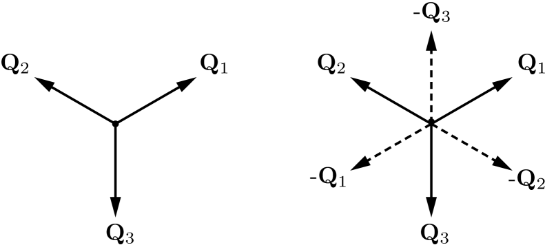
Figure 2: The multispiral (”3Q”) SkL structure in reciprocal space. Right-hand side of the figure shows the auxiliary negative reflexes, so that the hexagonal real-space SkL is built on the six wave vectors $\{\mathbf{Q}_{1},\text{-}\mathbf{Q}_{3},\mathbf{Q}_{2},\text{-}\mathbf{Q}_{1},\mathbf{Q}_{3},\text{-}\mathbf{Q}_{2}\}$, see the main text.

$$\mathcal{H}=\mathcal{H}_{JDh}+\mathcal{H}_{A}+\mathcal{H}_{\alpha E},$$ (2)

where the helimagnetic term

$$\mathcal{H}_{JDh}=J(\nabla\mathbf{S})^{2}+D\mathbf{S}\cdot(\nabla\times\mathbf{S})-\mathbf{h}\cdot\mathbf{S}$$ (3)

takes into account Heisenberg interaction ($J$), Dzialoshinskiy-Moriya interaction ($D$) and the Zeeman coupling to the external magnetic field $\mathbf{h}$. This coarse-grained model works when the following hierarchy of energies is respected: (1) the strongest is Heisenberg exchange parameter $J$ which favors the ferromagnetic alignment; (2) the Dzialoshinskiy-Moriya interaction (DMI) is slightly tilting two adjacent spins thus resulting helical modulations. (3) The cubic magnetocrystalline anisotropy $\mathcal{H}_{A}$ is considered the weakest in this hierarchy. Finally, the weak magnetoelectric term $\mathcal{H}_{\alpha E}$ is perturbatively small as estimated further. The spatial modulation of the ordered phase (the wavelength of the helices in the ground state) is given by a wave length of order $\lambda/a\sim J/D\gg 1$, i.e. much larger than the crystal lattice parameter $a$: for example, in ${\text{Cu}_{2}\text{O}\text{Se}\text{O}_{3}}$, $\lambda=630\,\text{\AA}$, $a=8.9\,\text{\AA}$, which gives $\lambda/a\sim 70$. In such case, the magnetization on neighboring lattice sites is varying very slowly and the physics of the system in the ordered phase is appropriately described by a continuous-limit model as assumed in (3).

In this study, we consider the fourth-order anisotropy as it represents the essential physics of the problem by stabilizing the SkL phase.White2014 ; Muhlbauer2009 The symmetry of ${\text{Cu}_{2}\text{O}\text{Se}\text{O}_{3}}$ is described by the $P2_{1}3$ space group, which allows a fourth-order magneto-crystalline anisotropy of the form $A_{1}(S_{x}^{4}+S_{y}^{4}+S_{z}^{4})+A_{2}(S_{x}^{2}S_{y}^{2}+S_{y}^{2}S_{z}^{2}+S_{z}^{2}S_{x}^{2})$, which can be reduced to

$$\mathcal{H}_{A}=A(S_{x}^{4}+S_{y}^{4}+S_{z}^{4}).$$ (4)

Indeed, proceeding to the unitary parametrization $\mathbf{S}/|\mathbf{S}|=(\sin\theta\cos\psi,\sin\theta\sin\psi,\cos\theta)$, one obtains $S_{x}^{2}S_{y}^{2}+S_{y}^{2}S_{z}^{2}+S_{z}^{2}S_{x}^{2}=-\frac{1}{2}(S_{x}^{4}+S_{y}^{4}+S_{z}^{4})+\frac{1}{2}$, thus $A=A_{1}-A_{2}/2$.

The magneto-electric coupling arises due to the weak $p$-$d$ hybridization mechanism(see Refs. Seki2012 ; Liu2013 ; Nagaosa2007 ; Belesi2012 ), which gives rise to an electric dipole moment $\mathbf{P}=\alpha_{\lambda}(S_{y}S_{z},S_{z}S_{x},S_{x}S_{y})$, i.e. the electric dipole moment coupled to the spin variables $S_{x},S_{y},S_{z}$. Therefore, in external electric fields the ordered phase is perturbed by $-\mathbf{P}\cdot\mathbf{E}$, or

$$\mathcal{H}_{\ae}=\alpha E_{x}S_{y}S_{z}+\text{cyclic permutations},$$ (5)

where $\mathbf{E}=(E_{x},E_{y},E_{z})$ is the external electric field and for simplicity we absorbed the minus sign into $\alpha=-\alpha_{\lambda}$. For ${\text{Cu}_{2}\text{O}\text{Se}\text{O}_{3}}$ the strength of magneto-electric coupling is estimated as $|\alpha|\sim 10^{-33}\,\text{Jm}/\text{V}$, see Ref.Omrani2014 .

The above expressions (3)-(5) are written in the natural frame. Experimentally, one often needs to apply magnetic and electric fields along directions where particular properties of the system are better revealed. In particular, in some $E$-field rotation experiments,White2014 the magnetic field $\mathbf{h}$ is parallel to $[1\,\bar{1}\,0]$, while the electric field is parallel to $[111]$ or $[\bar{1}\bar{1}\bar{1}]$, with $|E_{x}|=|E_{y}|=|E_{z}|\equiv E$ for simplicity of notations (thus the magnitude is $|\mathbf{E}|=\sqrt{3}E$). It is easier to carry out calculations in the rotated spin frame $(x^{\prime},y^{\prime},z^{\prime})$, with $\hat{z}^{\prime}$ set by the direction of magnetic field $\mathbf{h}$, see Fig. 3. In the case of above-mentioned geometry (Fig. 3), the transformation of the rotated spin frame is given by the rotation matrix

$$\begin{split}\begin{gathered}\mathcal{R}=\frac{1}{\sqrt{2}}\left(\begin{array}[]{ccc}1&0&1\\ 1&0&{\text{-}}1\\ 0&\sqrt{2}&0\end{array}\right).\end{gathered}\end{split}$$ (6)

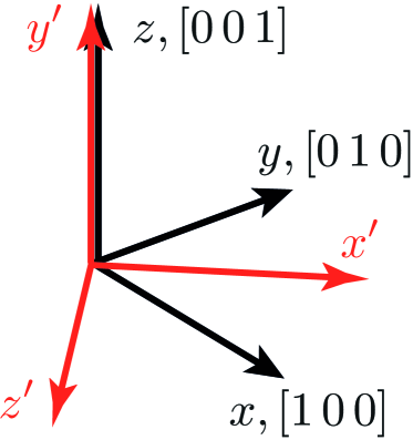
Figure 3: Rotated spin frame (red) for the magnetic field orientation $[1\,\bar{1}\,0]$.

While the helimagnetic term (3) is a Lifshitz invariant, the fourth-order anisotropy (4) is transformed under rotation (6) into

$$\begin{split}\begin{gathered}\mathcal{H}_{A}=A\left(\frac{1}{2}S_{x^{\prime}}^{4}+S_{y^{\prime}}^{4}+3S_{x^{\prime}}^{2}S_{z^{\prime}}^{2}+\frac{1}{2}S_{z^{\prime}}^{4}\right),\end{gathered}\end{split}$$ (7)

The $E$-field perturbation (5) also transforms under rotation ${\mathcal{R}}$,

$$\begin{split}\begin{gathered}\mathcal{H}_{\ae}=\frac{\alpha E}{2}\left(S_{x^{\prime}}^{2}+2\sqrt{2}S_{x^{\prime}}S_{y^{\prime}}-S_{z^{\prime}}^{2}\right),\end{gathered}\end{split}$$ (8)

and the electric field is directed along $\hat{e}_{x^{\prime}}+\hat{e}_{y^{\prime}}$. For simplicity, we drop the prime signs in the subsequent calculations.

We make a remark on the importance of the fourth-order magnetocrystalline anisotropy (4). The appearance of the $3{\mathbf{Q}}$-structure with ${\mathbf{Q}}_{1}+{\mathbf{Q}}_{2}+{\mathbf{Q}}_{3}=0$ with helices phased in a way to form the two-dimensional skyrmion crystalline occur only due to higher-order energy terms represented in the model. In chiral ferromagnets, the anisotropy of at least the fourth order can be considered as the source of the SkL order parameter. Indeed, we can consider the fourth order anisotropy which contains - fully or partially - the term $\mathbf{S}^{4}({\mathbf{r}})=S_{x}^{4}+S_{y}^{4}+S_{z}^{4}+2(S_{x}^{2}S_{y}^{2}+S_{y}^{2}S_{z}^{2}+S_{z}^{2}S_{x}^{2})$. Introducing now new variable without uniform magnetization $\mathbf{s}(\mathbf{r})=\mathbf{S}(\mathbf{r})-\mathbf{m}$, the fourth-order term will contain a cubic term

$$\begin{split}\begin{gathered}\mathbf{S}^{4}({\mathbf{r}})=\left[\mathbf{s}({\mathbf{r}})+\mathbf{m}\right]^{4}=...+4\mathbf{s}^{2}({\mathbf{r}})\,\mathbf{s}({\mathbf{r}})\cdot\mathbf{m}+...,\end{gathered}\end{split}$$ (9)

where we have not mentioned the other terms (linear, quadratic, quartic). The spatial average of the cubic term in the left-hand side of (9) can be Fourier-transformed as

$$\mathbf{m}\langle\mathbf{s}^{2}({\mathbf{r}})\,\mathbf{s}({\mathbf{r}})\rangle =\sum_{\mathbf{k}_{1,2,3}}(\mathbf{S}_{{\mathbf{k}}_{1}}\cdot\mathbf{S}_{{\mathbf{k}}_{2}})(\mathbf{m}\cdot\mathbf{S}_{{\mathbf{k}}_{3}})e^{i(\varphi_{{\mathbf{k}}_{1}}+\varphi_{{\mathbf{k}}_{2}}+\varphi_{{\mathbf{k}}_{3}})}$$ (10)

$$\times\mu^{3}\,\delta({\mathbf{k}}_{1}+{\mathbf{k}}_{2}+{\mathbf{k}}_{3}),$$ (11)

where $S_{{\mathbf{k}}}$ and their phases are defined as in Eq.(1), and ${\mathbf{k}}_{1,2,3}$ can be in principle any wave vector. If we define parameters in such a way that $\mu>0$, $(\mathbf{S}_{{\mathbf{k}}_{1}}\cdot\mathbf{S}_{{\mathbf{k}}_{2}})(\mathbf{m}\cdot\mathbf{S}_{{\mathbf{k}}_{3}})>0$, the hexagonal phase will be minimized if only $\varphi_{{\mathbf{k}}_{1}}+\varphi_{{\mathbf{k}}_{2}}+\varphi_{{\mathbf{k}}_{3}}=\pi$ and ${\mathbf{k}}_{1}+{\mathbf{k}}_{2}+{\mathbf{k}}_{3}=0$. The latest condition gives the so called $3\mathbf{Q}$ structure, ${\mathbf{Q}}_{1}+{\mathbf{Q}}_{2}+{\mathbf{Q}}_{3}=0$, with the three wave vectors equirotated by $2\pi/3$ due to symmetry.Muhlbauer2009 ; Binz2006 This situation is shown on Fig. 1.

II Skyrmion lattice in zero electric field: mean-field treatment

In this section we consider the mean-field treatment of the skyrmion lattice. First, we find the single-helix eigenstates, which give rise to a modulated spin structures with wave length $\lambda=2\pi/k_{0}=4\pi J/D$. After that, we construct the skyrmion lattice order parameter, and calculate the mean-field energy of the skyrmion lattice.

We start from considering the interplay between the Heisenberg term and the DMI coupling,

$$W_{0}=\langle J\left[\nabla\mathbf{S({\mathbf{r}})}\right]^{2}+D\,\mathbf{S}({\mathbf{r}})\cdot\left[\nabla\times\mathbf{S}({\mathbf{r}})\right]\rangle=\sum_{\mathbf{k}}\mathbf{S}_{{\mathbf{k}}}^{{\dagger}}\hat{\mathcal{H}}_{0}\mathbf{S}_{{\mathbf{k}}},$$ (12)

where in we used the Fourier transform of the spatial average to reciprocal space. Here $\hat{\mathcal{H}}_{0}$ is written in spin representation $\mathbf{S}_{{\mathbf{k}}}=(S_{\mathbf{k}}^{x},S_{\mathbf{k}}^{y},S_{\mathbf{k}}^{z})^{T}$ as a matrix operator

$$\begin{split}\begin{gathered}\hat{\mathcal{H}}_{0}=\left(\begin{array}[]{ccc}Jk^{2}&\text{-}iDk_{z}&iDk_{y}\\ iDk_{z}&Jk^{2}&\text{-}iDk_{x}\\ \text{-}iDk_{y}&iDk_{x}&Jk^{2}\end{array}\right).\end{gathered}\end{split}$$ (13)

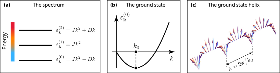
Figure 4: Appearance of the helical modulation: (a) The spectrum of $3\times 3$ energy matrix $\hat{\cal{H}}_{0}$. (b) Minimization of the state with lowest energy $\varepsilon^{(0)}_{{\mathbf{k}}}=Jk^{2}-Dk$ gives helix wave vector $k_{0}=D/2J$. (c) Real-space visualization of the helix with $\lambda=2\pi/k_{0}$.

The propagation vectors skyrmion lattice lie in the plane which is perpendicular to the magnetic field $\mathbf{h}$. Consequently, each of the six helices of the skyrmion lattice is parametrized as ${\mathbf{k}}=(k_{z},k_{y},0)$ in the rotated frame, thus the problem is effectively two-dimensional. The energy matrix (”hamiltonian”) (13) is

$$\begin{split}\begin{gathered}\hat{\mathcal{H}}_{0}=\left(\begin{array}[]{ccc}Jk^{2}&0&iDk_{y}\\ 0&Jk^{2}&\text{-}iDk_{x}\\ \text{-}iDk_{y}&iDk_{x}&Jk^{2}\end{array}\right),\end{gathered}\end{split}$$ (14)

and is diagonalized on the eigenstates

$$|\mathbf{S}^{(0)}_{{\mathbf{k}}}\rangle =\frac{1}{\sqrt{2}}\left(\text{-}i\hat{k}_{y},i\hat{k}_{x},1\right)^{\intercal},$$ (15)

$$|\mathbf{S}^{(1)}_{{\mathbf{k}}}\rangle =\left(\hat{k}_{x},\hat{k}_{y},0\right)^{\intercal},$$ (16)

$$|\mathbf{S}^{(2)}_{{\mathbf{k}}}\rangle =\frac{1}{\sqrt{2}}\left(i\hat{k}_{y},\text{-}i\hat{k}_{x},1\right)^{\intercal},$$ (17)

where $\hat{k}_{x,y,z}=k_{x,y,z}/|\mathbf{k}|$ and we introduced ”bra” and ”ket” notations as shortcuts to write the perturbation formulas of the matrix mechanics Green1965 in a familiar way. Consistent with our previous notations, we denote $\langle\mathbf{S}_{\mathbf{k}}|...|\mathbf{S}_{\mathbf{k}}\rangle=\sum_{\mathbf{k}}\mathbf{S}_{{\mathbf{k}}}^{{\dagger}}...\mathbf{S}_{{\mathbf{k}}}$, which is just a Fourier-transform of the corresponding spatial averaging $\langle...\rangle$ as in Eq.(12).

The spectrum of matrix $\hat{\mathcal{H}}_{0}$ consists of the three equidistant energy solutions, with the energy separation $\pm Dk$, see Fig. 4a,

$$\varepsilon^{(0)}_{{\mathbf{k}}}=Jk^{2}-Dk,\ \ \ \ \varepsilon^{(1)}_{{\mathbf{k}}}=Jk^{2},\ \ \ \ \varepsilon^{(2)}_{{\mathbf{k}}}=Jk^{2}+Dk,$$ (18)

For the positive $J$, $D$ the lowest energy solution is the helix

$$\begin{split}\begin{gathered}|\mathbf{S}^{(0)}_{{\mathbf{k}}}\rangle=\frac{1}{\sqrt{2}}\left(\begin{array}[]{c}\text{-}i\hat{k}_{y}\\ i\hat{k}_{x}\\ 1\end{array}\right),\end{gathered}\end{split}$$ (19)

which corresponds to the eigenvalue $\varepsilon^{(0)}_{{\mathbf{k}}}$. The modulation vector $k_{0}$ is determined by further minimization of the energy, ${\partial\varepsilon^{(0)}_{{\mathbf{k}}}}/{\partial k}=0$. Consequently, the minimum of the dispersion $\varepsilon^{(0)}_{{\mathbf{k}}}=Jk^{2}-Dk$ is satisfied if

$$k_{0}=\frac{D}{2J},$$ (20)

see also Fig. 3a,b. Finally, it is instructive to rewrite one more time the eigenspectrum of $\mathcal{H}_{0}$ as we use it in perturbation formulas further,

$$\varepsilon^{(0)}_{{\mathbf{k}}_{0}}=-Dk_{0}/2,\ \ \ \varepsilon^{(1)}_{{\mathbf{k}}_{0}}=Dk_{0}/2,\ \ \ \varepsilon^{(2)}_{{\mathbf{k}}_{0}}=3Dk_{0}/2.$$ (21)

As a remark, it is usually convenient to measure the energy of the system in units of $Dk_{0}$.

Next we consider the superposition of helices into a skyrmion lattice. Neglecting higher-order harmonics, the skyrmion lattice is approximated as uniform magnetization $m\hat{e}_{z}$ along magnetic field and a 3$Q$ multispiral configuration,

$$\mathbf{S}({\mathbf{r}})\simeq\mu\sum_{i=1}^{3}\left(\mathbf{S}_{\mathbf{Q}_{i}}e^{\mathbf{Q}_{i}{\mathbf{r}}}+c.c.\right)+m\,\hat{e}_{z}.$$ (22)

In the ”braket” notation, the real-space skyrmion phase has a shortcut notation

$$\begin{split}\begin{gathered}|\mathbf{S}({\mathbf{r}})\rangle=\mu\sum_{{\mathbf{k}}}^{\{\pm{\mathbf{Q}}_{1}...\pm{\mathbf{Q}}_{3}\}}|\mathbf{S}^{(0)}_{{\mathbf{k}}}\rangle e^{i{\mathbf{k}}{\mathbf{r}}+i\varphi_{{\mathbf{k}}}}+m|\mathbf{S}_{0}\rangle,\end{gathered}\end{split}$$ (23)

where $|\mathbf{S}^{(0)}_{{\mathbf{k}}}\rangle$ is given by Eq.(19) and the ferromagnetic component is $|\mathbf{S}_{0}\rangle\equiv(0\,0\,1)^{\intercal}$.

The skyrmion lattice possess some interesting properties. First, using the explicit form (22), the first-order moments are

$$\begin{split}\begin{gathered}\langle S_{x}({\mathbf{r}})\rangle=0,\ \ \ \langle S_{y}({\mathbf{r}})\rangle=0,\ \ \ \langle S_{z}({\mathbf{r}})\rangle=m,\end{gathered}\end{split}$$ (24)

so the uniform magnetization (the ”ferromagnetic component”) $\mathbf{m}\equiv\langle\mathbf{S}({\mathbf{r}})\rangle=m\,\hat{e}_{z}$ is the only non-vanishing first-order moment. The second-order in-plane moments are

$$\langle S_{x}^{2}({\mathbf{r}})\rangle =\sum^{\left\{{\mathbf{q}}_{1}...{\mathbf{q}}_{6}\right\}}_{{\mathbf{k}}}S^{x}_{{\mathbf{k}}}S^{x}_{-{\mathbf{k}}}=3\mu^{2}/2,$$ (25)

$$\langle S_{y}^{2}({\mathbf{r}})\rangle =\sum^{\left\{{\mathbf{q}}_{1}...{\mathbf{q}}_{6}\right\}}_{{\mathbf{k}}}S^{y}_{{\mathbf{k}}}S^{y}_{-{\mathbf{k}}}=3\mu^{2}/2,$$ (26)

while the longitudinal (z) second-order moment is

$$\begin{split}\begin{gathered}\langle S_{z}^{2}({\mathbf{r}})\rangle=m^{2}+\sum^{\left\{{\mathbf{q}}_{1}...{\mathbf{q}}_{6}\right\}}_{{\mathbf{k}}}S^{z}_{{\mathbf{k}}}S^{z}_{-{\mathbf{k}}}=m^{2}+3\mu^{2}.\end{gathered}\end{split}$$ (27)

One can verify that all the mixed moments vanish,

$$\langle S_{\alpha}S_{\beta}\rangle=0,\ \ \ \alpha\neq\beta,$$ (28)

so, in general, one has

$$\langle S_{\alpha}S_{\beta}\rangle=\frac{3}{2}\mu^{2}\delta_{\alpha,\beta}[1+(1+2m^{2}/3\mu^{2})\delta_{\alpha,z}],$$ (29)

where $\alpha,\beta={x,y,z}$. Formula (29) is handy for further expectation value calculations. For a fixed temperature one can use normalization $\langle\mathbf{S}^{2}({\mathbf{r}})\rangle=1$, thus the following constraint holdsWhite2014

$$\langle\mathbf{S}^{2}\rangle=m^{2}+6\mu^{2}=1.$$ (30)

Finally, it is interesting to note that in this approximation the fourth-order moment for the skyrmion lattice is surprisingly $\langle\mathbf{S}^{4}\rangle\neq\langle\mathbf{S}^{2}\rangle^{2}$, i.e. the magnetization field is “soft”.

Now we consider the skyrmion lattice in finite magnetic fields by adding the source term $-\mathbf{h}\cdot\mathbf{S}$,

$$W^{(h)}_{0} =\langle J\left[\nabla\mathbf{S({\mathbf{r}})}\right]^{2}+D\,\mathbf{S}({\mathbf{r}})\cdot\left[\nabla\times\mathbf{S}({\mathbf{r}})\right]-\mathbf{h}\cdot\mathbf{S}({\mathbf{r}})\rangle$$ (31)

$$=\sum^{\left\{{\mathbf{q}}_{1}...{\mathbf{q}}_{6}\right\}}_{\mathbf{k}}\mathbf{S}_{{\mathbf{k}}}^{{\dagger}}\ \hat{\mathcal{H}}_{0}\ \mathbf{S}_{{\mathbf{k}}}-h\,m,$$

which however doesn’t change the mean-field eigenstates (15)-(17) as it contains no spatial derivatives. Thus the expectation value (31) is modified only in terms of elongating the ferromagnetic component $m$, but the topology of the skyrmion order parameter is not affected. The mean-field treatment of the SkL energy (31) yields

$$\begin{split}\begin{gathered}W^{(h)}_{0}=-3Dk_{0}\,\mu^{2}-h\,m.\end{gathered}\end{split}$$ (32)

In the mean-field treatment, one may minimize the total energy with respect to all the components of the magnetic moment, including $m$ and $\mu$, if a comparison between two phases is needed. For example, minimizing now Eq.(32) with constraint (30), one gets the mean-field estimates $m_{\text{MF}}=h/Dk_{0}$ and $\mu_{\text{MF}}=\sqrt{(1-m_{\text{MF}}^{2})/6}$. The corresponding energy is therefore given as $W^{(h)}_{0}=-Dk_{0}\left(m^{2}_{\text{MF}}+1\right)/2$.

Finally, we calculate perturbatively the anisotropic contribution around the mean-field. For the anisotropy of form (4) (without spatial derivatives), the wave vectors of helices are not renormalized. Therefore, the contribution of anisotropy to the energy of the skyrmion lattice is calculated by using the same order parameter (23). Decoupling the ferromagnetic contribution $\mathbf{m}$ from Eq.(7), one obtains

$$\langle{\cal H}_{A}\rangle =\frac{1}{2}Am^{4}+A\langle\frac{1}{2}s_{x}^{4}+s_{y}^{4}+3s_{x}^{2}s_{z}^{2}+\frac{1}{2}s_{z}^{4}\rangle$$ (33)

$$+Am\langle 6s_{x}^{2}s_{z}+2s_{z}^{3}\rangle+Am^{2}\langle 3s_{x}^{2}+3s_{z}^{2}\rangle.$$

A direct calculation within the unperturbed state Eq.(23) gives

$$\langle{\cal H}_{A}\rangle =\frac{1}{2}Am^{4}+\frac{27}{2}Am^{2}\mu^{2}+\frac{963}{32}A\mu^{4}$$ (34)

$$+\frac{21}{\sqrt{2}}A\mu^{3}m\cos(\varphi_{1}+\varphi_{2}+\varphi_{3}).$$

Note that the term containing $\mu^{3}$, is responsible for the minimization of the $3Q$ structure, as was discussed in Section I. For $A>0$, $m>0$, $\mu>0$, expression (34) is minimized for $\varphi_{1}+\varphi_{2}+\varphi_{3}=\pi$, which gives

$$\langle{\cal H}_{A}\rangle_{0}=\frac{1}{2}Am^{4}+\frac{27}{2}Am^{2}\mu^{2}-\frac{21}{\sqrt{2}}A\mu^{3}m+\frac{963}{32}A\mu^{4}.$$ (35)

The energy of the skyrmion lattice in the absence of electric field is thus given by (32) and (35) in the mean-field approximation.

III Skyrmion Lattice in Electric Fields: Elastic distortion

In this section we consider the shift in the SkL energy caused by distortion of the skyrmion vectors. We start by re-writing the magneto-electric coupling in the rotated frame (8) in symmetrized form, which in units $Dk_{0}$ is simply

$$\begin{split}\begin{gathered}\hat{\mathcal{H}}_{\ae}/Dk_{0}=2\ae\left(\begin{array}[]{ccc}1&\sqrt{2}&0\\ \sqrt{2}&0&0\\ 0&0&\text{-}1\end{array}\right),\end{gathered}\end{split}$$ (36)

where we have introduced the dimensionless electric field æ,

$$\begin{split}\begin{gathered}\ae\equiv\frac{\alpha E}{4Dk_{0}},\end{gathered}\end{split}$$ (37)

which plays the role of the small parameter of the theory. To illustrate its smallness, we use typical electric fields $E=5\times 10^{6}\,\text{V/m}$, and ${\text{Cu}_{2}\text{O}\text{Se}\text{O}_{3}}$ parameters as $J=4.85\times 10^{-23}\,\text{Jm}/\text{A}$, $k_{0}=D/2J=10^{8}\,\text{m}$, and ME couplingMochizuki2015 is $\alpha\sim 10^{-14}\,\text{J}/\text{m}^{2}\text{V}$. This gives $\ae\sim 0.01$. Thus throughout this study, we build the perturbation theory in orders of $\ae^{1}$ and $\ae^{2}$, which is sufficient for describing both the symmetric and asymmetric responses in $E$-fields.

First, we consider the helix vectors in external electric field. Considering $E$-field as a small perturbation (36) on top of the $JD$-matrix (14), matrix perturbation theory givesGreen1965

$$\begin{split}\begin{gathered}|{\mathbf{S}}^{(\ae)}_{\mathbf{k}}\rangle=|{\mathbf{S}}^{(0)}_{\mathbf{k}}\rangle+\sum_{n\neq 0}|{\mathbf{S}}^{(n)}_{\mathbf{k}}\rangle\frac{\langle{\mathbf{S}}^{(n)}_{\mathbf{k}}|\hat{\mathcal{H}}_{\ae}|{\mathbf{S}}^{(0)}_{\mathbf{k}}\rangle}{\varepsilon^{(0)}_{\mathbf{k}}-\varepsilon^{(n)}_{{\mathbf{k}}}}+{\mathcal{O}}(\ae^{2}).\end{gathered}\end{split}$$ (38)

where $\varepsilon^{(n)}_{{\mathbf{k}}}$ are given by Eq.(21) and $|{\mathbf{S}}^{(n)}_{\mathbf{k}}\rangle$, $n=0,1,2$, are eigenstates of $\mathcal{H}_{0}$ as given by Eqs.(14-16). The perturbed helix (38) is by construction normalized on unity up to terms of order ${\mathcal{O}}(\ae^{2})$,

$$\langle{\mathbf{S}}^{(\ae)}_{\mathbf{k}}|{\mathbf{S}}^{(\ae)}_{\mathbf{k}}\rangle=1+\mathcal{O}(\ae^{2}).$$ (39)

A direct calculation for the new helix, using formulas (38), (36), (15)-(17), gives

$$\begin{split}\begin{gathered}|{\mathbf{S}}^{(\ae)}_{\mathbf{k}}\rangle=|{\mathbf{S}}^{(0)}_{\mathbf{k}}\rangle-\ae\,|{\mathbf{F}}_{{\mathbf{k}}}\rangle+{\mathcal{O}}(\ae^{2}),\end{gathered}\end{split}$$ (40)

where ${\mathbf{F}}_{{\mathbf{k}}}={\mathbf{F}}(\hat{k}_{x},\hat{k}_{y})\equiv{\mathbf{F}}_{\mathbf{k}}(\phi)$ is the elastic distortion vector (here for each helix $\hat{k}_{x}=\cos\phi$, $\hat{k}_{y}=\sin\phi$, that is $\phi$ is angle between $\mathbf{k}$ and $\hat{x}$), so that

$$\begin{split}\begin{gathered}|{\mathbf{F}}_{\mathbf{k}}\rangle=\left(iF^{x}_{{\mathbf{k}}}(\phi),iF^{y}_{{\mathbf{k}}}(\phi),F^{z}_{{\mathbf{k}}}(\phi)\right)^{\intercal},\end{gathered}\end{split}$$ (41)

with angle-dependent components

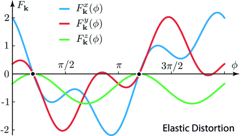
Figure 5: Components of elastic distortion vector $\mathbf{F}_{{\mathbf{k}}}$ as functions of the helix angle $\phi$. $F_{{\mathbf{k}}}^{x,y}$ are $2\pi$-periodic while $F_{{\mathbf{k}}}^{z}$ is $\pi$-periodic. The dots denote stationary points which are not effected by $E$-field.

$$F^{x}_{{\mathbf{k}}}(\phi) =-\frac{\sin\phi}{\sqrt{2}}+2\cos^{3}\phi-\frac{3\sin\phi\cos^{2}\phi}{2\sqrt{2}}-\sin^{2}\phi\,\cos\phi,$$ (42)

$$F^{y}_{{\mathbf{k}}}(\phi) =\frac{\cos\phi}{2\sqrt{2}}-2\sin^{3}\phi+\sin\phi\cos^{2}\phi-\frac{3\sin^{2}\phi\,\cos\phi}{2\sqrt{2}},$$ (43)

$$F^{z}_{{\mathbf{k}}}(\phi) =-\frac{1}{2\sqrt{2}}-\frac{\sin^{2}\phi}{2\sqrt{2}}+\sin\phi\cos\phi.$$ (44)

The components $F^{x}_{{\mathbf{k}}}$, $F^{y}_{{\mathbf{k}}}$, $F^{x}_{{\mathbf{k}}}$ of the elastic distortion vector are $\pi$ and $2\pi$ periodic functions, and are illustrated in Fig. 6. Note that the $x$ and $y$ components of both ${\mathbf{S}}^{(0)}_{\mathbf{k}}$ and ${\mathbf{S}}^{(\ae)}_{\mathbf{k}}$ are imaginary, and $z$ component is real for both ${\mathbf{S}}^{(0)}_{\mathbf{k}}$ and ${\mathbf{S}}^{(\ae)}_{\mathbf{k}}$. Physically it means that the field-induced distortion of the skyrmion lattice does not change the orientation of the skyrmion plane. One can verify both analytically and numerically that Eqs.(42)-(43) together with (41) satisfy normalization (39).

IV Energy shift of the Skyrmion Lattice in Electric Fields

In this section, we calculate the shift of the SkL energy in the first two orders in terms of dimensionless electric field $\ae$. This shift is contributed by the expectation value of the magnetoelectric coupling, and the anisotropic contributions due to the skyrmion lattice distortion.

IV.1 Magneto-Electric Response

The first contribution to the energy shift of the skyrmion lattice in electric field comes from taking the expectation value of (36) in the appropriate order in $\ae$. In this study, we consider $\ae$ to be small, thus the second order is sufficient for capturing the essential physics in both antisymmetric (field reversion $E\to-E$ gives the energy shifts of different signs) and symmetric (field reversion $E\to-E$ gives the energy shifts of same signs) cases of interest. Using the explicit expression (40)–(44), one obtains

$$\begin{split}\begin{gathered}\langle\hat{\mathcal{H}}_{\ae}\rangle/Dk_{0}=-(2m^{2}+3\mu^{2})\,\ae-\frac{189}{4}\mu^{2}\ae^{2}+\mathcal{O}(\ae^{3}).\end{gathered}\end{split}$$ (45)

The expression (45) is the leading contribution in case if the anisotropy of the system is small. Restoring the dimensional units, the shift of the SkL energy $W$ in electric field $E$ is therefore given by

$$\Delta W_{1}(E)= -\frac{\alpha(2m^{2}+3\mu^{2})M_{s}^{2}a^{3}}{4}E$$ (46)

$$-\frac{189\,\alpha^{2}\mu^{2}M_{s}^{2}a^{3}}{64\,Dk_{0}}E^{2}+\mathcal{O}(E^{3}).$$

where $M_{s}$ is saturation magnetization (in $\text{A}/\text{m}$), $a$ is the lattice constant. Note that the helimagnetic term $H_{JDh}$ is not giving shift contributions to this order.

IV.2 Anisotropy response

Now, we calculate the direct contribution of anisotropy to the energy shift. The main physical mechanism here is the distortion of SkL in electric field, which results to perturbation in the anisotropic energy. To proceed, we explicitly use formulas (40)–(44) to calculate the expectation value of the anisotropic term in the new ground state. In the leading order one therefore obtains

$$\langle{\cal H}_{A}\rangle_{1}=\langle\mathbf{S}^{(\ae)}|\hat{\cal H}_{A}|\mathbf{S}^{(\ae)}\rangle\simeq\frac{9}{8}Am^{2}\mu^{2}\,\ae+\frac{99}{32}A\mu^{4}\,\ae$$ (47)

$$+\frac{81}{64}A\mu^{4}\,\ae\,(\cos 6\phi_{0}+2\sqrt{2}\sin 6\phi_{0})$$

$$+\frac{27}{4\sqrt{2}}A\,\ae\,m\mu^{3}\cos(\varphi_{1}+\varphi_{2}+\varphi_{3}).$$

Here $\phi_{0}$ is the angle between the first skyrmion helix and $\hat{x}$ (note that due to $2\pi/3$ symmetry in SkL rotation, and $6\phi$-arguments in Eq.(47), one can take $\phi_{0}$ as the angle between any of the skyrmion helices and $\hat{x}$). The same angular dependence [third term in Eq.(47)] were reported in study White2014 , where the minimization of SkL energy in electric fields leads to the SkL rotation in real space with respect to $\hat{x}$, if six-order anisotropy is considered, however all the angular-independent anisotropic contributions were there neglected.White2014 We notice that expression (47) is dependent on the relative phases of the helices $\varphi_{i}$. The same situation occurs in (34), when the mean-field energy is dependent on phase. We take again $\cos(\varphi_{1}+\varphi_{2}+\varphi_{3})=-1$, which minimizes the mean-field energy for fixed positive $m$, $\mu$, therefore

$$\langle{\cal H}_{A}\rangle_{1} =\frac{9}{8}A\mu^{4}\left(\frac{11}{4}-3\sqrt{2}\frac{\mu}{m}+\frac{\mu^{2}}{m^{2}}\right)\ae$$ (48)

$$+\frac{81}{64}A\mu^{4}(\cos 6\phi_{0}+2\sqrt{2}\sin 6\phi_{0})\,\ae+\mathcal{O}(\ae^{2}).$$

This contribution gives the linear anisotropic response to the external field. However, for the completeness of discussion, we need to take into account further terms $\mathcal{O}(\ae^{2})$, which come both from the elastic distortion of the SkL and the inelastic (quadratic in $\ae$) distortion of the SkL.

IV.2.1 Mixed Inelastic response

To consider the nonlinear anisotropic response, we re-define the perturbed helix eigenstates up to the second order, which are given by a perturbative expansion

$$|{\mathbf{S}}^{(\ae)}_{\mathbf{k}}\rangle=|{\mathbf{S}}^{(0)}_{\mathbf{k}}\rangle+\sum_{n\neq 0}|{\mathbf{S}}^{(n)}_{\mathbf{k}}\rangle\frac{\langle{\mathbf{S}}^{(n)}_{\mathbf{k}}|\hat{\mathcal{H}}_{PE}|{\mathbf{S}}^{(0)}_{\mathbf{k}}\rangle}{\varepsilon^{(0)}_{\mathbf{k}}-\varepsilon^{(n)}_{{\mathbf{k}}}}$$ (49)

$$+\sum_{n,m\neq 0}|{\mathbf{S}}^{(n)}_{\mathbf{k}}\rangle\frac{\langle{\mathbf{S}}^{(n)}_{\mathbf{k}}|\hat{\mathcal{H}}_{\ae}|{\mathbf{S}}^{(m)}_{\mathbf{k}}\rangle\langle{\mathbf{S}}^{(m)}_{\mathbf{k}}|\hat{\mathcal{H}}_{\ae}|{\mathbf{S}}^{(0)}_{\mathbf{k}}\rangle}{(\varepsilon^{(0)}_{\mathbf{k}}-\varepsilon^{(n)}_{{\mathbf{k}}})\,(\varepsilon^{(0)}_{\mathbf{k}}-\varepsilon^{(m)}_{{\mathbf{k}}})}$$

$$-\sum_{n\neq 0}|{\mathbf{S}}^{(n)}_{\mathbf{k}}\rangle\frac{\langle{\mathbf{S}}^{(n)}_{\mathbf{k}}|\hat{\mathcal{H}}_{\ae}|{\mathbf{S}}^{(0)}_{\mathbf{k}}\rangle\langle{\mathbf{S}}^{(0)}_{\mathbf{k}}|\hat{\mathcal{H}}_{\ae}|{\mathbf{S}}^{(0)}_{\mathbf{k}}\rangle}{(\varepsilon^{(0)}_{\mathbf{k}}-\varepsilon^{(n)}_{{\mathbf{k}}})^{2}}$$

$$-\frac{1}{2}\sum_{n\neq 0}|{\mathbf{S}}^{(0)}_{\mathbf{k}}\rangle\frac{\langle{\mathbf{S}}^{(0)}_{\mathbf{k}}|\hat{\mathcal{H}}_{\ae}|{\mathbf{S}}^{(n)}_{\mathbf{k}}\rangle\langle{\mathbf{S}}^{(n)}_{\mathbf{k}}|\hat{\mathcal{H}}_{\ae}|{\mathbf{S}}^{(0)}_{\mathbf{k}}\rangle}{(\varepsilon^{(0)}_{\mathbf{k}}-\varepsilon^{(n)}_{{\mathbf{k}}})^{2}}$$

$$+{\mathcal{O}}(\ae^{3}).$$

This expansion leads to re-definition of (40) by adding a nonelastic distortion of the skyrmion lattice,

$$\begin{split}\begin{gathered}|{\mathbf{S}}^{(\ae)}_{\mathbf{k}}\rangle=|{\mathbf{S}}^{(0)}_{\mathbf{k}}\rangle-\ae\,|{\mathbf{F}}_{{\mathbf{k}}}\rangle+\ae^{2}\,|{\mathbf{G}}_{{\mathbf{k}}}\rangle+{\mathcal{O}}(\ae^{3}),\end{gathered}\end{split}$$ (50)

where ${\mathbf{G}}_{{\mathbf{k}}}={\mathbf{G}}(\hat{k}_{x},\hat{k}_{y})\equiv{\mathbf{G}}_{\mathbf{k}}(\phi)$ is the main inelastic distortion vector,

$$\begin{split}\begin{gathered}|{\mathbf{G}}_{\mathbf{k}}\rangle=\left(iG^{x}_{{\mathbf{k}}}(\phi),iG^{y}_{{\mathbf{k}}}(\phi),G^{z}_{{\mathbf{k}}}(\phi)\right)^{T}.\end{gathered}\end{split}$$ (51)

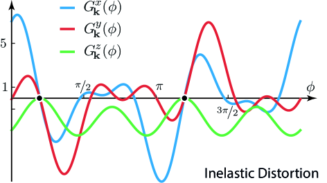
Figure 6: Components of the nonelastic distortion vector $\mathbf{G}_{\mathbf{k}}$ as a function of the helix direction angle $\phi$. $G_{{\mathbf{k}}}^{x,y}$ are $2\pi$-periodic while $G_{{\mathbf{k}}}^{z}$ is $\pi$-periodic. The dots denote stationary points which are not effected by $E$-field.

The direct calculation of the inelastic distortion vector, by using (49), (36), (15)-(17), gives

$$G^{x}_{{\mathbf{k}}}(\phi) =-\frac{39}{64\sqrt{2}}\sin\phi+\frac{131}{128\sqrt{2}}\sin 3\phi+\frac{273}{128\sqrt{2}}\sin 5\phi$$ (52)

$$+\frac{33}{16}\cos\phi+\frac{119}{32}\cos 3\phi+\frac{39}{32}\cos 5\phi,$$

$$G^{y}_{{\mathbf{k}}}(\phi) =-\frac{33}{16}\sin\phi+\frac{37}{32}\sin 3\phi+\frac{39}{32}\sin 5\phi$$

$$-\frac{93}{64\sqrt{2}}\cos\phi+\frac{443}{128\sqrt{2}}\cos 3\phi-\frac{273}{128\sqrt{2}}\cos 5\phi,$$

$$G^{z}_{{\mathbf{k}}}(\phi) =\frac{3}{8}\sin 2\phi+\frac{15}{16}\sin 4\phi+\frac{3}{16\sqrt{2}}\cos 2\phi$$

$$-\frac{105}{64\sqrt{2}}\cos 4\phi-\frac{171}{64\sqrt{2}}.$$

These dependencies are shown in Fig.6. The comparison between the elastic and inelastic distortion vectors is shown on Figure 7. Finally, for the numerical consistence of calculations, one can verify that the new ground state is normalized on unity,

$$\langle{\mathbf{S}}^{(\ae)}_{\mathbf{k}}|{\mathbf{S}}^{(\ae)}_{\mathbf{k}}\rangle=1+\mathcal{O}(\ae^{3}).$$ (53)

Therefore, the mixed elastic-inelastic response $\mathcal{O}(\ae^{2})$ is obtained by calculating the expectation value in the new basis (50). The direct calculation gives

$$\langle{\cal H}_{A}\rangle_{2}=\frac{27}{64}A\mu^{4}\left(f_{0}+f_{1}\cos 6\phi_{0}+f_{2}\sin 6\phi_{0}\right)\ae^{2},$$ (54)

where we have introduced the following dimensionless factors

$$f_{0} =-\frac{191}{8}+62\sqrt{2}\,\frac{m}{\mu}-16\frac{m^{2}}{\mu^{2}},$$ (55)

$$f_{1} =29-14\sqrt{2}\,\frac{m}{\mu}+56\frac{m^{2}}{\mu^{2}},$$ (56)

$$f_{2} =-59\sqrt{2}+16\frac{m}{\mu}-32\sqrt{2}\,\frac{m^{2}}{\mu^{2}}.$$ (57)

The mixed elastic-inelastic contribution (54) gives the second-order correction in $\ae$ which may be important in some particular cases, for example, when the first order correction vanishes. Then, the electric field response does not depend on the field polarity ($\pm E$ is absorbed in $E^{2}$).

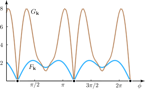
Figure 7: Comparison between magnitudes of elastic $F_{{\mathbf{k}}}=\left|\mathbf{F}_{{\mathbf{k}}}\right|$ and nonelastic $G_{{\mathbf{k}}}=\left|\mathbf{G}_{{\mathbf{k}}}\right|$ distortion vectors as the function of the helix angle $\phi$. There $\pi$-periodic stationary points, which indicate the direction along which the helices are not disturbed, $F_{k}=G_{k}=0$.

Therefore, we have three contributions to the shift in the SkL mean-field energy:

$$\Delta W_{1}(E)=-\frac{\alpha(2m^{2}+3\mu^{2})M_{s}^{2}a^{3}}{4}E-\frac{189\,\alpha^{2}\mu^{2}M_{s}^{2}a^{3}}{64\,Dk_{0}}E^{2},$$ (58)

$$\Delta W_{2}(E)=\frac{9\alpha\,A\mu^{4}M_{s}^{2}a^{3}}{32Dk_{0}}E\left[\frac{11}{4}-3\sqrt{2}\frac{\mu}{m}+\frac{\mu^{2}}{m^{2}}\right.$$ (59)

$$\left.+\frac{9}{8}(\cos 6\phi_{0}+2\sqrt{2}\sin 6\phi_{0})\right],$$

$$\Delta W_{3}(E) =\frac{27\alpha^{2}A\mu^{4}M_{s}^{2}a^{3}}{1024\,D^{2}k_{0}^{2}}E^{2}$$ (60)

$$\times\left(f_{0}+f_{1}\cos 6\phi_{0}+f_{2}\sin 6\phi_{0}\right).$$

Together, formulas (58)-(60) give the contribution up to the second order in electric field $E$. In case of the weak anisotropy $A\ll D^{2}/J$, the term (60) can be usually neglected. Note also that in the main-order approximation ($\ae^{1}$) the $E$-field induced shift in energy is also the shift in free energy of the skyrmion lattice for a fixed temperature near $T_{C}$.

It is therefore possible to stabilize (if $\Delta W_{\text{total}}<0$) or destabilize (if $\Delta W_{\text{total}}>0$) the skyrmion lattice by choosing the appropriate magnitudes and polarities of electric fields. This coincides with the previous idea of Mochizuki Mochizuki2016 of creating single magnetic skyrmions with external $E$-fields in multiferroic ${\text{Cu}_{2}\text{O}\text{Se}\text{O}_{3}}$. The present study is therefore a bridge towards this idea in the bulk samples, where the skyrmions usually exist in the form of long-range-ordered or partially-disordered skyrmion arrays. The experimental research into writing and erasing skyrmions with electric fields in bulk ${\text{Cu}_{2}\text{O}\text{Se}\text{O}_{3}}$ is on the final stage in our lab and will be published elsewhere.

V Summary

The present model describes the shift of the mean-field energy of the SkL, which is either positive or negative depending on the direction of the electric field. In a particular situation, when the first order terms vanish, the energy shift is of the same sign for both field polarities.

An interesting output of the calculation is the existence of the stationary points if a helix is directed in a proper way (Fig. 7). This feature comes both in the elastic and nonelastic distortions of the skyrmion lattice. However, as the SkL is constructed on the three helices, the mean-field energy of the SkL is still shifted.

Finally, we sketch the limitations of the calculation. First, this study describes the first two perturbative corrections to the mean-field energy of the skyrmion lattice in the multispiral approximation, without comparing the free energies of different possible phases (helical, conical) in the system. Second, the energy functional is taken in the quasiclassical continuous-field limit, which limits the use of the model only to the sufficiently low DMI parameter ($D/J\ll 1$) and excludes the quantum regime (low $T$). Third, the effect of electric field on critical fluctuations on top of the mean-field SkL solution is not considered as it comes as a higher-order contribution in the critical correlation length.

The main physical consequence of the phenomenon under study is the field-induced stabilization of the skyrmion phase in the bulk, which has been so far indirectly observed in ${\text{Cu}_{2}\text{O}\text{Se}\text{O}_{3}}$. Okamura2016 This mechanism if further developed would allow one either to write or erase the skyrmion array over the full sample if it is properly placed in the $H$, $T$ phase diagram, and thus opens further routes for skyrmion-based racetrack logical elements and data storage devices.

Acknowledgments. - The work was supported by the Swiss National Science Foundation, its Sinergia network Mott Physics Beyond the Heisenberg Model (MPBH). The authors would like to thank Achim Rosch and Jiadong Zang for useful discussion.

References

- (1) A. N. Bogdanov and D. A. Yablonskii, Sov. Phys. JETP, 95 (1989).
- (2) B. Binz, A. Vishwanath, V. Aji, Phys. Rev. Lett. 96, 207202 (2006).
- (3) S. Muhlbauer, B. Binz, F. Jonietz, C. Pfleiderer, A. Rosch, A. Neubauer, R. Georgii, P. Boni, Science 323, 5916 (2009)
- (4) T. H. R. Skyrme, Proc. Roy. Soc. Lon. 260, 127 (1961).
- (5) A. Fert, V. Cros and J. Sampaio, Nature Nanotechnology 8, 152156 (2013).
- (6) N. Nagaosa and Y. Tokura, Nature Nanotechnology 8, 899911 (2013).
- (7) R. Tomasello, E. Martinez, R. Zivieri, L. Torres, M. Carpentieri and G. Finocchio, Scientific Reports 4, 6784 (2014).
- (8) X. Zhang, G. P. Zhao, Hans Fangohr, J. Ping Liu, W. X. Xia, J. Xia, F. J. Morvan, Scientific Reports 5, 7643 (2015).
- (9) X. Zhang, M. Ezawa and Y. Zhou, Scientific Reports 5, 9400 (2015).
- (10) A. Tonomura, X. Yu, K. Yanagisawa, T. Matsuda, Y. Onose, N. Kanazawa, H. S. Park, and Y. Tokura, Nano Lett., 12 (3), (2012).
- (11) W. Munzer, A. Neubauer, T. Adams, S. Muhlbauer, C. Franz, F. Jonietz, R. Georgii, P. Boni, B. Pedersen, M. Schmidt, A. Rosch, and C. Pfleiderer, Phys. Rev. B 81, 041203(R) (2010).
- (12) Y. Tokunaga, X. Z. Yu, J. S. White, H. M. Ronnow, D. Morikawa, Y. Taguchi and Y. Tokura, Nature Communications 6, 7638 (2015).
- (13) T. Adams, A. Chacon, M. Wagner, A. Bauer, G. Brandl, B. Pedersen, H. Berger, P. Lemmens, and C. Pfleiderer, Phys. Rev. Lett. 108, 237204 (2012).
- (14) J. S. White, I. Levatic, A. A. Omrani, N. Egetenmeyer, K. Prsa, I Zivkovic, J. L. Gavilano, J. Kohlbrecher, M. Bartkowiak, H. Berger and and H. M. Rønnow, Journal of Physics: Condensed Matter, 24, 43 (2012).
- (15) J. S. White, K. Prsa, P. Huang, A. A. Omrani, I. Zivkovic, M. Bartkowiak, H. Berger, A. Magrez, J. L. Gavilano, G. Nagy, J. Zang, and H. M. Ronnow, Phys. Rev. Lett. 113, 107203 (2014).
- (16) I. Levatic, P. Popcevic, V. Surija, A. Kruchkov, H. Berger, A. Magrez, J. S. White, H. M. Ronnow, I. Zivkovic, Scientific Reports 6, 21347 (2016).
- (17) Y. Okamura, F. Kagawa, S. Seki, and Y. Tokura, Nature Communications 7, 12669 (2016).
- (18) F. Jonietz, S. Muhlbauer, C. Pfleiderer, A. Neubauer, W. Munzer, A. Bauer, T. Adams, R. Georgii, P. Bni, R. A. Duine, et al., Science 330, 1648 (2010).
- (19) X. Z. Yu, N. Kanazawa, W. Z. Zhang, T. Nagai, T. Hara, K. Kimoto, Y. Matsui, Y. Onose, and Y. Tokura, Nature Communications 3, 988 (2012).
- (20) W. Jiang, P. Upadhyaya, W. Zhang, G. Yu, M. B. Jungfleisch, F. Y. Fradin, J. E. Pearson, Y. Tserkovnyak, K. L. Wang, O. Heinonen, et al., Science 349, 283 (2015).
- (21) K. Everschor, M. Garst, B. Binz, F. Jonietz, S. Muhlbauer, C. Pfleiderer and A. Rosch, Phys. Rev. B 86, 054432 (2012).
- (22) H. Watanabe, A. Vishwanath, J. Phys. Soc. Jpn. 85, 064707 (2016)
- (23) M. Mochizuki, X. Z. Yu, S. Seki, N. Kanazawa, W. Koshibae, J. Zang, M. Mostovoy, Y. Tokura, and N. Nagaosa, Nature Materials 13, 241 (2014).
- (24) S. Seki, X.Z. Yu, S. Ishiwata, and Y. Tokura, Science, 336 (6078), 198-201 (2012).
- (25) M. Mochizuki and Y. Watanabe, Applied Physics Letters 107, 082409 (2015).
- (26) M. Mochizuki, Advanced Electronic Materials 2 (2016).
- (27) A. A. Omrani, J. S. White, K. Prsa, I. Zivkovic, H. Berger, A. Magrez, Ye-Hua Liu, J. H. Han, and H. M. Ronnow Phys. Rev. B 89, 064406 (2014).
- (28) M. Mochizuki and Y. Watanabe, Appl. Phys. Lett. 107, 082409 (2015).
- (29) P. Upadhyaya, G. Yu, P. K. Amiri, and K. L. Wang Phys. Rev. B 92, 134411 (2015)
- (30) S. Seki, S. Ishiwata, and Y. Tokura, Phys. Rev. B 86, 060403(R) (2012).
- (31) Y.-H. Liu, Y.-Q. Li, and J. H. Han, Phys. Rev. B 87, 100402 (2013).
- (32) M. Belesi, I. Rousochatzakis, M. Abid, U. K. Rossler, H. Berger, and J.-Ph. Ansermet, Phys. Rev. B 85, 224413 (2012).
- (33) C. Jia, S. Onoda, N. Nagaosa, and J. H. Han, Phys. Rev. B 76, 144424 (2007).
- (34) B. Binz and A. Vishwanath, Physica B: Cond. Matt. 403, 5 (2008).
- (35) H.S. Green, Matrix mechanics, P. Noordhoff, (1965).
- (36) M. Janoschek, M. Garst, A. Bauer, P. Krautscheid, R. Georgii, P. Boni, and C. Pfleiderer, Phys. Rev. B 87, 134407 (2013).