Millimeter Wave Beam-Selection Using Out-of-Band Spatial Information

Abstract

Millimeter wave (mmWave) communication is one feasible solution for high data-rate applications like vehicular-to-everything communication and next generation cellular communication. Configuring mmWave links, which can be done through channel estimation or beam-selection, however, is a source of significant overhead. In this paper, we propose to use spatial information extracted at sub-$6\text{\,}\mathrm{GHz}$ to help establish the mmWave link. First, we review the prior work on frequency dependent channel behavior and outline a simulation strategy to generate multi-band frequency dependent channels. Second, assuming: (i) narrowband channels and a fully digital architecture at sub-$6\text{\,}\mathrm{GHz}$; and (ii) wideband frequency selective channels, OFDM signaling, and an analog architecture at mmWave, we outline strategies to incorporate sub-$6\text{\,}\mathrm{GHz}$ spatial information in mmWave compressed beam-selection. We formulate compressed beam-selection as a weighted sparse signal recovery problem, and obtain the weighting information from sub-$6\text{\,}\mathrm{GHz}$ channels. In addition, we outline a structured precoder/combiner design to tailor the training to out-of-band information. We also extend the proposed out-of-band aided compressed beam-selection approach to leverage information from all active OFDM subcarriers. The simulation results for achievable rate show that out-of-band aided beam-selection can reduce the training overhead of in-band only beam-selection by $4$x.

I Introduction

Millimeter wave (mmWave) communication systems use large antenna arrays and directional beamforming/precoding to provide sufficient link margin [2, 3]. Large arrays are feasible at mmWave as antennas can be packed into small form factors. Configuring these arrays, however, is not without challenges. First, the high power consumption of RF components makes fully digital baseband precoding difficult [2]. Second, the precoder design usually relies on channel state information, which is difficult to acquire at mmWave due to large antenna arrays and low pre-beamforming signal-to-noise ratio (SNR). Thus, mmWave link establishment has received considerable research interest [4, 5, 6, 7, 8]. The usual strategy is to exploit some sort of structure in the unknown channel that aids in link establishment, e.g., sparsity [4, 5] or channel dynamics [6].

Beyond leveraging the structure in the mmWave channel, it is possible to exploit out-of-band (OOB) information extracted from sub-6 $\text{\,}\mathrm{GHz}$ channels for mmWave link establishment. This is relevant as mmWave systems will likely be deployed in conjunction with lower frequency systems: (i) to provide wide area control signals; and/or (ii) for multi-band communications [9, 10]. In this work, we propose to use the sub-6 $\text{\,}\mathrm{GHz}$ spatial information as OOB side information about the mmWave channel. This is feasible as the spatial characteristics of sub-6 $\text{\,}\mathrm{GHz}$ and mmWave channels are similar [11]. Extracting spatial information from sub-6 $\text{\,}\mathrm{GHz}$ is also enticing due to favorable receive SNR in comparison with mmWave. The benefit of using sub-6 $\text{\,}\mathrm{GHz}$ information in mmWave link establishment has been demonstrated through measurements in [12].

OOB information has the potential to reduce the training overhead of mmWave link establishment (be it through channel estimation [4] or beam-selection [5]). As such, using OOB information can have a positive impact on all mmWave communication applications. It is, however, especially interesting in high mobility scenarios where frequent link reconfiguration is required. Here, we highlight the benefits in two specific use cases i.e., vehicle-to-everything (V2X) communication and mmWave cellular.

To increase driving automation, next generation vehicles will boast more and better sensors. The sensing ability of a vehicle can be supplemented by exchanging sensor data with other vehicles and infrastructure. Such exchange, however, is data-rate hungry, as sensors may generate up to hundreds of $\text{\,}\mathrm{Mbps}$ [13]. The current vehicular communication mechanisms do not support such data-rates. For example, dedicated short-range communication (DSRC) [14] operates at 2-6 $\text{\,}\mathrm{Mbps}$, and practical rates of LTE-A are limited to several $\text{\,}\mathrm{Mbps}$ [15]. An amendment of the mmWave WLAN standard IEEE 802.11ad could provide a future framework for a high data-rate V2X communication system, in a similar way as IEEE 802.11p was considered for DSRC. There is also a growing body of research on mmWave vehicular communications (see e.g., [16, 17] and the references therein). The highly dynamic nature of V2X channels, however, requires frequent link configuration and OOB-aided link establishment can play an important role in unlocking the potential of mmWave V2X. As an example, the OOB information for mmWave V2X links could come from the DSRC channels or automotive sensors.

Due to the large bandwidths available in the mmWave spectrum and the directional nature of mmWave communications, implying less interference and high data-rate gains, mmWave frequencies are also promising for future outdoor cellular systems [18, 2, 19]. Channel measurements have confirmed that mmWave is feasible for both access and backhaul links [8, 3]. In addition, the system level evaluation of mmWave network performance has indicated that mmWave cellular systems achieve a spectral efficiency similar to sub-6 $\text{\,}\mathrm{GHz}$ [20]. Understanding these benefits, the Federal Communications Commission (FCC) has proposed rules to make mmWave spectrum available for mobile cellular services [21]. At large distances, e.g., cell edges, the pre-beamforming SNR is very low and establishing a reliable mmWave link is particularly challenging. As SNR for sub-6 $\text{\,}\mathrm{GHz}$ sytems is more favorable, reliable OOB information from sub-6 $\text{\,}\mathrm{GHz}$ can be used to aid the mmWave link establishment.

In this work, we use the sub-6 $\text{\,}\mathrm{GHz}$ spatial information for mmWave link establishment. Specifically, we consider the problem of finding the optimal transmit/receive beam-pair for analog mmWave systems. We assume wideband frequency selective MIMO channels and OFDM signaling for the analog mmWave system. For sub-6 $\text{\,}\mathrm{GHz}$, we assume narrowband MIMO channels and a fully digital architecture. Both sub-6 $\text{\,}\mathrm{GHz}$ and mmWave systems use uniform linear arrays (ULAs) at the transmitter (TX) and the receiver (RX). The main contributions of this work are:

• Based on the review of prior work, we draw conclusions about the expected degree of congruence between sub-6 $\text{\,}\mathrm{GHz}$ and mmWave systems. The term “spatial congruence” is used to describe the similarity in the power distribution of arrival/departure angles of the channels. We outline a simulation strategy to generate multi-band frequency dependent channels that are consistent with frequency-dependent channel behavior observed in prior work.

• We propose a procedure to leverage OOB spatial information in compressed beam-selection [5] for an analog mmWave architecture. Specifically, exploiting the limited scattering nature of mmWave channels and using the training on one OFDM subcarrier, we formulate the beam-selection as a weighted sparse signal recovery problem [22]. The weights are chosen based on the OOB information. Further, we suggest a structured random codebook design. The proposed design enforces the training precoder/combiner patterns to have high gains in the strong channel directions based on OOB information.

• We formulate the compressed beam-selection as a multiple measurement vector (MMV) sparse recovery problem [23] to leverage training from all active subcarriers. The MMV based sparse recovery improves the beam-selection by a simultaneous recovery of multiple sparse signals with common support. We extend the weighted sparse recovery and structured codebook design to the MMV case.

Prior work on using OOB information in communication systems primarily targets beamforming reciprocity in frequency division duplex (FDD) systems. Based on the observation that the spatial information in the uplink (UL) and downlink (DL) is congruent [24, 25], several correlation translation strategies were proposed to estimate DL correlation from UL measurements (see e.g., [26, 27] and references therein). The estimated correlation was in turn used for DL beamforming. Along similar lines, in [28] the multi-paths in the UL channel were estimated and subsequently the DL channel was constructed using the estimated multi-paths. In [29], the UL measurements were used as partial support information in compressed sensing based DL channel estimation. The frequency separation between UL and DL is typically small. As an example, there is $9.82\%$ frequency separation between $1935\text{\,}\mathrm{MHz}$ UL and $2125\text{\,}\mathrm{MHz}$ DL [25]. The aforementioned strategies were tailored for the case when the percent frequency separation of the channels under consideration is small and spatial information is congruent. In this work, we consider channels that can have frequency separation of several hundred percent, and hence some degree of spatial disagreement is expected.

There is some prior work on leveraging OOB information for mmWave communications. In [12], the directional information from legacy WiFi was used to reduce the beam-steering overhead of $60\text{\,}\mathrm{GHz}$ WiFi. The measurement results presented in [12] confirm the value of OOB information for mmWave link establishment. This work is distinguished from [12] as the techniques developed in this work are applicable to non line-of-sight (NLOS) channels, whereas [12] primarily considered LOS channels. In [30], correlation translation strategies were presented to estimate mmWave correlation using sub-6 $\text{\,}\mathrm{GHz}$ correlation. The estimated correlation was in turn used for linear channel estimation in SIMO systems. In contrast with [30], we consider MIMO systems and focus on compressed beam-selection in an analog architecture. The concept of radar aided mmWave communication was introduced in [31]. The information extracted from a mmWave radar was used to configure the mmWave communication link. Unlike [31], we use sub-6 $\text{\,}\mathrm{GHz}$ communication system’s information for mmWave link establishment.

This work is an extension of [1] and provides a detailed treatment of the problem. Herein, we propose and use a frequency dependent clustered channel model, where each cluster contributes multiple rays. The clustered behavior is observed in recent mmWave channel modeling studies [32]. In contrast, [1] assumed that each cluster contributes a single ray. Further, this work considers frequency selective wideband channels for mmWave, whereas [1] assumed a narrowband channel. Finally, we present a structured random codebook design that is not present in [1].

The rest of the paper is organized as follows: In Section II, we review the prior work on frequency dependent channel behavior and outline a simulation strategy to generate multi-band frequency dependent channels. In Section III, we provide the system and channel models for sub-6 $\text{\,}\mathrm{GHz}$ and mmWave systems. In Section IV, we outline strategies to incorporate the OOB information in compressed beam-selection. The simulation results are presented in Section V, and Section VI concludes the paper.

Notation: We use the following notation throughout the paper. Bold lowercase ${\mathbf{x}}$ is used for column vectors, bold uppercase ${\mathbf{X}}$ is used for matrices, non-bold letters $x$, $X$ are used for scalars. $[{\mathbf{x}}]_{m}$, $[{\mathbf{X}}]_{m,n}$, $[{\mathbf{X}}]_{m,:}$, and $[{\mathbf{X}}]_{:,n}$, denote $m$th entry of ${\mathbf{x}}$, entry at the $m$th row and $n$th column of ${\mathbf{X}}$, $m$th row of ${\mathbf{X}}$, and $n$th column of ${\mathbf{X}}$, respectively. Superscript ${\sf T}$ and $\ast$ represent the transpose and conjugate transpose. ${\mathbf{0}}$ and ${\mathbf{I}}$ denote the zero vector and identity matrix respectively. $\mathcal{C}\mathcal{N}({\mathbf{x}},{\mathbf{X}})$ denotes a complex circularly symmetric Gaussian random vector with mean ${\mathbf{x}}$ and correlation ${\mathbf{X}}$. We use ${\mathbb{E}}[\cdot]$, $\|\!\cdot\!\|_{p}$, and $\|\!\cdot\!\|_{\mathrm{F}}$ to denote expectation, $p$ norm and Frobenius norm, respectively. ${\mathbf{X}}\otimes{\mathbf{Y}}$ is the Kronecker product of ${\mathbf{X}}$ and ${\mathbf{Y}}$. Calligraphic letter $\mathcal{X}$ denotes sets and $[X]$ represents the set $\{1,2,\cdots,X\}$. Finally, $|\!\cdot\!|$ is the absolute value of its argument or the cardinality of a set, and ${\rm vec}(\cdot)$ yields a vector for a matrix argument. The sub-6 $\text{\,}\mathrm{GHz}$ variables are underlined, as $\underline{{\mathbf{x}}}$, to distinguish them from mmWave.

II Multi-band channel characteristics and simulation

The OOB-aided mmWave beam-selection strategies proposed in this work rely on the information extracted at sub-6 $\text{\,}\mathrm{GHz}$. Therefore, it is essential to understand the similarities and differences between sub-6 $\text{\,}\mathrm{GHz}$ and mmWave channels. Furthermore, to assess the performance of proposed OOB-aided mmWave link establishment strategies, a simulation strategy is required to generate multi-band frequency dependent channels. In this section, we review a representative subset of prior work to draw conclusions about the expected degree of spatial congruence between sub-6 $\text{\,}\mathrm{GHz}$ and mmWave channels. Based on these results, we outline a strategy to simulate multi-band frequency dependent channels.

Due to the differences in the wavelength of sub-6 $\text{\,}\mathrm{GHz}$ and mmWave frequencies, it is possible that the Fresnel zone clarity criterion for LOS is satisfied at sub-6 $\text{\,}\mathrm{GHz}$ but not for mmWave. It is expected that the OOB-aided link establishment will not perform well in such scenarios as the spatial information in a LOS sub-6 $\text{\,}\mathrm{GHz}$ and NLOS mmWave may be different. One can venture to detect such scenarios and revert to in-band only link establishment. The authors defer this issue to future work.

II-A Review of multi-band channel characteristics

The material properties change with frequency, e.g., the relative conductivity and the average reflection increase with frequency [33, 34]. Hence, some characteristics of the channel are expected to vary with frequency. It was reported that the delay spread decreases [35, 36, 37, 38], the number of angle-of-arrival (AoA) clusters increase [32], the shadow fading increases [37], and the angle spread (AS) of clusters decreases [38, 36] with frequency. Further, it was observed that the late arriving multi-paths have more frequency dependence due to higher interactions with the environment [39, 40].

Not all channel characteristics vary greatly with frequency. As an example, the existence of spatial congruence between the UL and DL channels is well established [24, 25]. In [24], it was noted that though the propagation channels in UL and DL are not reciprocal, the spatial information is congruent. It was observed in measurements (for $1935\text{\,}\mathrm{MHz}$ UL and $2125\text{\,}\mathrm{MHz}$ DL) that the deviation in AoAs of dominant paths of UL and DL is small with high probability [25]. Prior work has exploited the spatial congruence between UL and DL channels to reduce/eliminate the feedback in FDD systems, see e.g., [26, 27, 28, 29].

Some channel characteristics are congruent for larger frequency separations. In [11], the directional power distribution of $5.8$ $\text{\,}\mathrm{GHz}$, $14.8$ $\text{\,}\mathrm{GHz}$, and $58.7$ $\text{\,}\mathrm{GHz}$ LOS channels were reported to be almost identical. The number of resolvable paths, the decay constants of the clusters, the decay constants of the subpaths within the clusters, and the number of angle-of-departure (AoD) clusters were found to be similar in $28$ and $73$ $\text{\,}\mathrm{GHz}$ channels [32]. In [41], similar power delay profiles (PDP)s were reported for $10$ $\text{\,}\mathrm{GHz}$ and $30$ $\text{\,}\mathrm{GHz}$ channels. The received power as a function of distance was found to be similar for $5.8$ $\text{\,}\mathrm{GHz}$ and $14.8$ $\text{\,}\mathrm{GHz}$ in [11]. Only minor differences were observed in the CDFs of delay spread, azimuth AoA/AoD spread, and elevation AoA/AoD spread of six different frequencies between $2\leavevmode\nobreak\ $\text{\,}\mathrm{GHz}$$ and $60$ $\text{\,}\mathrm{GHz}$ in [42].

In conclusion, the prior work confirms that there is substantial similarity between channels at different frequencies, even with large separations. Hence, it is likely that there is significant, albeit not perfect, congruence between sub-6 $\text{\,}\mathrm{GHz}$ and mmWave channels. This observation is leveraged by prior work that used legacy WiFi measurements to configure $60\leavevmode\nobreak\ $\text{\,}\mathrm{GHz}$$ WiFi links [12].

II-B Simulation of multi-band frequency dependent channels

The following observations are made about the frequency dependent channel behavior from the review of the prior work:

• The channel characteristics differ with frequency, and the differences increase as the percent separation between center frequencies of the channels increase.

• The late arriving multi-paths have more frequency dependence [39, 40], and some paths may be present at one frequency but not at the other [43].

The proposed multi-band frequency dependent channel simulation algorithm takes the aforementioned observations into consideration. It takes the parameters of the channels at two frequencies as input and outputs a random realization for each of the two channels. The input parameters include the number of clusters, the number of paths within a cluster, maximum delay spread, root mean squared (RMS) time spread of the paths within clusters, center frequency, and the RMS AS of the paths within clusters. The output random realizations of the two channels are consistent in the sense that one of the channels is a perturbed version of the other, where the perturbation model respects the frequency dependent channel behavior. Before discussing the proposed simulation algorithm, we present the required preliminaries.

The following exposition is applicable to the channels at two frequencies $f_{1}$ and $f_{2}$ (not necessarily sub-6 $\text{\,}\mathrm{GHz}$ and mmWave). Therefore, we use subscript index $i\in[I]$, where $I=2$, to distinguish the parameters of the channel at center frequency $f_{1}$ from the parameters of the channel at center frequency $f_{2}$. In subsequent sections, we use underlined and non-underlined analogs of the variables defined here for sub-6 $\text{\,}\mathrm{GHz}$ and mmWave, respectively. We assume that there are $C_{i}$ clusters in the channel $i$. Each cluster has a mean time delay $\tau_{c,i}\in[0,\tau_{\max,i}]$ and mean physical AoA/AoD $\{\theta_{c,i},\phi_{c,i}\}\in[0,2\pi)$. Each cluster $c_{i}$ is further assumed to contribute $R_{c,i}$ rays/paths between the TX and the RX. Each ray $r_{c,i}\in[R_{c,i}]$ has a relative time delay $\tau_{r_{c,i}}$, relative AoA/AoD shift $\{\vartheta_{r_{c,i}},\varphi_{r_{c,i}}\}$, and complex path gain $\alpha_{r_{c,i}}$. If $\rho_{{\mathrm{p}}{\mathrm{l}},i}$ represents the path-loss, then the omni-directional impulse response of the channel $i$ can be written as

$$h_{{\mathrm{o}}{\mathrm{m}}{\mathrm{n}}{\mathrm{i}},i}(t,\theta,\phi)=\dfrac{1}{\sqrt{\rho_{{\mathrm{p}}{\mathrm{l}},i}}}\sum_{c_{i}=1}^{C_{i}}\sum_{r_{c,i}=1}^{R_{c,i}}\alpha_{r_{c,i}}\delta(t-\tau_{c,i}-\tau_{r_{c,i}})\times\delta(\theta-\theta_{c,i}-\vartheta_{r_{c,i}})\times\delta(\phi-\phi_{c,i}-\varphi_{r_{c,i}}).$$ (1)

The continuous time channel impulse response given in (1) is not band-limited. The impulse response convolved with pulse shaping filter, however, is band-limited and can be sampled to obtain the discrete time channel as in Section III. Further, in (1) we have only considered the azimuth AoAs/AoDs for simplicity. The general formulation with both azimuth and elevation angles is a straightforward extension, see [32]. A detailed discussion on the choice of the channel parameters is beyond the scope of this paper. The reader is directed to prior work e.g., [44] for discussions on suitable channel parameters. A cursory guideline can be established, however, based on the literature review presented earlier. Assuming $f_{1}\leq f_{2}$ it is expected that $C_{1}\geq C_{2}$ [32], $R_{c,1}\geq R_{c,2}$ [32], $\tau_{\max,1}\geq\tau_{\max,2}$ [35, 36, 37, 38], $\sigma_{\vartheta_{c,1}}\geq\sigma_{\vartheta_{c,2}}$, and $\sigma_{\varphi_{c,1}}\geq\sigma_{\varphi_{c,2}}$ [38, 36]. Furthermore, the parameters used for numerical evaluations in Section V are an example of the parameters that comply with the observations of the prior work.

The proposed channel simulation strategy is based on a two-stage algorithm. In the first stage, the mean time delays $\tau_{c,i}$ and mean AoAs/AoDs $\{\theta_{c,i},\phi_{c,i}\}$ of the clusters are generated for both frequencies in a coupled manner, while respecting the frequency dependent behavior. In the second stage, the paths within the clusters are generated independently for both frequencies. The first stage of the proposed channel simulation algorithm is outlined in Algorithm 1.

II-B1 First Stage

The number of clusters $C_{i}$, the maximum delay spreads $\tau_{\max,i}$, and the center frequencies $f_{i}$ for channels $i\in[I]$ are fed to the first-stage of the proposed algorithm as inputs. The first stage has three parts. In the first part, the clusters for both the channels are generated independently. In the second part, we replace several clusters in one of the channels by the clusters of the other channel. The first two parts ensure that there are a few common as well as a few uncommon clusters in the channels. Finally, in the third part frequency dependent perturbations are added to the clusters of one of the channels. This is to imitate the effect that the common clusters in the two channels may have a time/angle offset.

Part 1: (Generation) The algorithm initially generates the mean time delays and mean AoAs/AoDs for the clusters i.e., $\{\tau_{c,i},\theta_{c,i},\phi_{c,i}\}$, $\forall c_{i}\in[C_{i}],\forall i\in[I]$. The set of the three parameters $\{\tau_{c,i},\theta_{c,i},\phi_{c,i}\}$ corresponding to a cluster is referred to as the cluster parameter set. The clusters for both channels are generated independently.

Part 2: (Replacement) We replace several clustes in one channel with the clusters of the other to esnure common clusters in the channels. This step is to be carried in accordance with the following observations: (i) the late arriving clustered paths are more likely to fade independently across the two channels [39, 40]; and (ii) independent clustered paths are more likely as the percent frequency separation increases. In other words, for fixed percent frequency separation, the early arriving clustered paths have a higher likelihood of co-occurrence in both channels. We store the indices of co-occuring clusters in sets $\mathcal{R}_{i},\forall i\in[I]$, henceforth called the replacement index sets. As an example, the index sets can be created by sorting the cluster parameter sets in an ascending order with respect to $\tau_{c,i}$ and populating $\mathcal{R}_{i}=\{i:\xi>\frac{|f_{i}-f_{[[I]\setminus i]}|}{\max(f_{i},f[[I]\setminus i])}\frac{\tau_{c,i}}{\tau_{\max,i}}\}$. Here $\xi$ is a standard Uniform random variable, i.e., $\xi\sim U[0,1]$. For the candidate indices that appear in $\mathcal{R}_{1}$ and $\mathcal{R}_{2}$, we replace the corresponding clusters in one channel with those of the other. Without loss of generality, we replace the clusters of the channel with larger delay spread. Hence, we update the cluster parameters sets $\{\tau_{c,b},\theta_{c,b},\phi_{c,b}\}\leavevmode\nobreak\ \forall c_{b}\in\mathcal{R}_{b}\cap\mathcal{R}_{[I]\setminus b}$ with $\{\tau_{c,[I]\setminus b},\theta_{c,[I]\setminus b},\phi_{c,[I]\setminus b}\}\leavevmode\nobreak\ \forall c_{[I]\setminus b}\in\mathcal{R}_{b}\cap\mathcal{R}_{[I]\setminus b}$, where $b=\underset{i}{\arg\max}\leavevmode\nobreak\ \tau_{\max,i}$.

Part 3: (Perturbation) So far we have simulated the effect that there will be common as well as uncommon clusters in the channels at two frequencies. Now we need to add frequency dependent perturbation in the clusters of one of the channels to simulate the behavior that co-occurring clusters can have some time/angle offset. The perturbation should be: (i) proportional to the mean time delay of the cluster [39, 40]; and (ii) proportional to percent center frequency separation. We continue by assuming that the clusters of the channel $b$ are perturbed. A scalar perturbation $\Delta_{c,b}$ is generated $\forall c_{b}\in[C_{b}]$. The perturbation $\Delta_{c,b}$ is then modified for delays and AoAs/AoDs using deterministic modifiers $g_{\tau}(\cdot)$, $g_{\theta}(\cdot)$ and $g_{\phi}(\cdot)$, respectively. The rationale of using deterministic modifications of the same perturbation for delays and angles is the coupling of these parameters in the physical channels. This is to say that the amount of variation in the mean delay of the cluster, from one frequency to another, is not expected to be independent of the variation in AoA/AoD. Let us define the function

$$q(x,w,y,z)=\begin{cases}1&\text{if }x-w<y,\\ -1&\text{if }x+w>z,\\ \pm 1\leavevmode\nobreak\ \text{with equal probability}&\text{otherwise}.\\ \end{cases}$$ (2)

With this definition, an example perturbation model could be $\Delta_{c,b}\sim U[0,1]$, $g_{\tau}(\Delta_{c,b})=q(\tau_{c,b},\Delta_{c,b},0,\tau_{\max,b})\frac{|f_{b}-f_{[I]\setminus b}|}{\max(f_{b},f_{[I]\setminus b})}\tau_{c,b}\Delta_{c,b}$ and $g_{\theta}(\Delta_{c,b})=q(\theta_{c,b},\Delta_{c,b},0,2\pi)\frac{|f_{b}-f_{[I]\setminus b}|}{\max(f_{b},f_{[I]\setminus b})}\frac{\tau_{c,b}}{\tau_{\max,b}}\Delta_{c,b}$. The modifier $g_{\phi}$ can be chosen similar to $g_{\theta}$. The modified perturbations $g_{\tau}(\Delta_{c,b})$, $g_{\theta}(\Delta_{c,b})$, and $g_{\phi}(\Delta_{c,b})$ are added in $\tau_{c,b}$, $\theta_{c,b}$, and $\phi_{c,b}$, respectively, to obtain the cluster parameters for channel $b$. Finally, the cluster parameter sets for both channels are returned.

Algorithm 1 Mean time delays $\tau_{c,i}$ and mean AoAs/AoDs $\{\theta_{c,i},\phi_{c,i}\}$ generation

1:$C_{i},\tau_{\max,i},f_{i},\leavevmode\nobreak\ \forall i\in[I]$

2:$\{\tau_{c,i},\theta_{c,i},\phi_{c,i}\}\leavevmode\nobreak\ \forall c_{i}\in[C_{i}],\forall i\in[I]$

3:Draw $\tau_{c,i}\sim U[0,\tau_{\max,i}],\{\theta_{c,i},\phi_{c,i}\}\sim U[0,2\pi)\leavevmode\nobreak\ \forall c_{i}\in[C_{i}],\forall i\in[I]$ to get the cluster parameter sets $\{\tau_{c,i},\theta_{c,i},\phi_{c,i}\}\leavevmode\nobreak\ \forall c_{i}\in[C_{i}],\forall i\in[I]$.

4:Populate replacement index sets $\mathcal{R}_{i},\forall i\in[I]$ using a suitable replacement model, and update $\{\tau_{c,b},\theta_{c,b},\phi_{c,b}\}\leavevmode\nobreak\ \forall c_{b}\in\mathcal{R}_{b}\cap\mathcal{R}_{[I]\setminus b}\leftarrow\{\tau_{c,[I]\setminus b},\theta_{c,[I]\setminus b},\phi_{c,[I]\setminus b}\}\leavevmode\nobreak\ \forall c_{[I]\setminus b}\in\mathcal{R}_{b}\cap\mathcal{R}_{[I]\setminus b}$, where $b=\underset{i}{\arg\max}\leavevmode\nobreak\ \tau_{\max,i}$.

5:Generate $C_{b}$ perturbations $\Delta_{c,b}$ and update $\tau_{c,b}\leftarrow\tau_{c,b}+g_{\tau}(\Delta_{c,b})$, $\theta_{c,b}\leftarrow\theta_{c,b}+g_{\theta}(\Delta_{c,b})$, and $\phi_{c,b}\leftarrow\phi_{c,b}+g_{\phi}(\Delta_{c,b})$.

II-B2 Second Stage

Once the parameters $\{\tau_{c,i},\theta_{c,i},\phi_{c,i}\},\forall c_{i}\in[C_{i}],\forall i\in[I]$ are available, the paths/rays within the clusters are generated independently for both channels in the second stage of the proposed algorithm. The second stage requires the number of paths per cluster $R_{c,i}$, the RMS time spread of the paths within clusters $\sigma_{\tau_{r_{c,i}}}$, and the RMS AS of the relative arrival and departure angle offsets $\{\sigma_{\vartheta_{c,i}},\sigma_{\varphi_{c,i}}\}$, as input. The output of the second stage are the sets $\{\alpha_{r_{c,i}},\tau_{r_{c,i}},\vartheta_{r_{c,i}},\varphi_{r_{c,i}}\},\leavevmode\nobreak\ \forall r_{c,i}\in R_{c,i},\forall i\in[I]$. The relative time delays $\tau_{r_{c,i}}$ are generated according to a suitable intra-cluster PDP (e.g., Exponential or Uniform), the relative angle shifts $\{\vartheta_{r_{c,i}},\varphi_{r_{c,i}}\}$ according to a suitable azimuth power spectrum (APS) (e.g., uniform, truncated Gaussian or truncated Laplacian), and the complex coefficients $\alpha_{r_{c,i}}$ according to a suitable fading model (e.g., Rayleigh or Ricean).

III System and channel model

We consider a multi-band MIMO system shown in Fig. 1, where ULAs of isotropic point sources are used at the TX and the RX. The ULAs are considered for ease of exposition, whereas, the proposed strategies can be extended to other array geometries with suitable modifications. We assume that the sub-6 $\text{\,}\mathrm{GHz}$ and mmWave arrays are co-located, aligned, and have comparable apertures. Both sub-6 $\text{\,}\mathrm{GHz}$ and mmWave systems operate simultaneously.

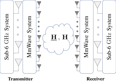
Figure 1: The multi-band MIMO system with co-located sub-6 $\text{\,}\mathrm{GHz}$ and mmWave antenna arrays. The sub-6 $\text{\,}\mathrm{GHz}$ channel is $\underline{{\mathbf{H}}}$ and the mmWave channel is ${\mathbf{H}}$.

III-A Sub-6 $\text{\,}\mathrm{GHz}$ system and channel model

The sub-6 $\text{\,}\mathrm{GHz}$ system is shown in Fig. 2. Note that, we underline all sub-6 $\text{\,}\mathrm{GHz}$ variables to distinguish them from the mmWave variables. The sub-6 $\text{\,}\mathrm{GHz}$ system has one RF chain per antenna and as such, fully digital precoding is possible. We assume narrowband signaling at sub-6 $\text{\,}\mathrm{GHz}$. Extending the proposed approach to wideband sub-6 $\text{\,}\mathrm{GHz}$ systems is straight forward because only the directional information is retrieved from sub-6 $\text{\,}\mathrm{GHz}$, which is not expected to vary much across the channel bandwidth. We adopt a geometric channel model for $\underline{{\mathbf{H}}}$ based on (1). The MIMO channel matrix for sub-6 $\text{\,}\mathrm{GHz}$ can be written as

$$\underline{{\mathbf{H}}}=\sqrt{\dfrac{\underline{M}_{{\mathrm{R}}{\mathrm{X}}}\underline{M}_{{\mathrm{T}}{\mathrm{X}}}}{\underline{\rho}_{{\mathrm{p}}{\mathrm{l}}}}}\sum_{\underline{c}=1}^{\underline{C}}\sum_{r_{\underline{c}}=1}^{\underline{R}_{\mathrm{c}}}\underline{\alpha}_{r_{\underline{c}}}p(-\underline{\tau}_{\underline{c}}-\underline{\tau}_{r_{\underline{c}}})\underline{{\mathbf{a}}}_{{\mathrm{R}}{\mathrm{X}}}(\underline{\theta}_{\underline{c}}+\underline{\vartheta}_{r_{\underline{c}}})\underline{{\mathbf{a}}}_{{\mathrm{T}}{\mathrm{X}}}^{\ast}(\underline{\phi}_{\underline{c}}+\underline{\varphi}_{r_{\underline{c}}}),$$ (3)

where $p(\tau)$ denotes a pulse shaping function evaluated at $\tau$ seconds, $\underline{{\mathbf{a}}}_{{\mathrm{R}}{\mathrm{X}}}(\theta)$ and $\underline{{\mathbf{a}}}_{{\mathrm{T}}{\mathrm{X}}}(\phi)$ are the antenna array response vectors of the RX and the TX, respectively. The array response vector of the RX is

$$\underline{{\mathbf{a}}}_{{\mathrm{R}}{\mathrm{X}}}(\theta)=\frac{1}{\sqrt{\underline{M}_{{\mathrm{R}}{\mathrm{X}}}}}[1,e^{{\rm j}2\pi\underline{d}\sin(\theta)},\cdots,e^{{\rm j}2\pi(\underline{M}_{{\mathrm{R}}{\mathrm{X}}}-1)\underline{d}\sin(\theta)}]^{\sf T},$$ (4)

where $\underline{d}$ is the inter-element spacing in wavelength. The array response vector of the TX is defined in a similar manner. The normalized spatial AoA of the sub-6 $\text{\,}\mathrm{GHz}$ system is $\underline{\nu}\triangleq\underline{d}\sin(\theta)$ and the spatial AoD is $\underline{\omega}\triangleq\underline{d}\sin(\phi)$.

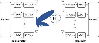
Figure 2: The sub-6 $\text{\,}\mathrm{GHz}$ system with digital precoding.

III-B Millimeter wave system and channel model

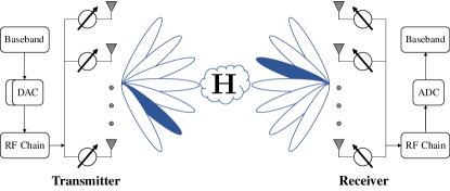
Figure 3: The mmWave system with phase-shifters based analog beamforming.

The mmWave system is shown in Fig. 3. The TX has $M_{{\mathrm{T}}{\mathrm{X}}}$ antennas and the RX has $M_{{\mathrm{R}}{\mathrm{X}}}$ antennas. Both the TX and the RX are equipped with a single RF chain, hence only analog beamforming is possible. The idea of using OOB information can also be applied to hybrid analog/digital and fully digital low-resolution mmWave architectures, an interesting direction for future work. The mmWave system uses OFDM signaling with $K$ subcarriers. The data symbols on each subcarrier ${\mathsf{s}}[k],\leavevmode\nobreak\ \forall k\in[K]$ are transformed to the time-domain using a $K$-point IDFT. A cyclic prefix (CP) of length $L_{{\mathrm{c}}}$ is then prepended to the time-domain samples before applying the analog precoder ${\mathbf{f}}$. The length $L_{{\mathrm{c}}}$ CP followed by the $K$ time-domain samples constitute one OFDM block. The effective transmitted signal on subcarrier $k$ is ${\mathbf{f}}{\mathsf{s}}[k]$. The data symbols follow ${\mathbb{E}}[{\mathsf{s}}[k]{\mathsf{s}}^{\ast}[k]]=\dfrac{P_{{\mathrm{t}}}}{K}$, where $P_{{\mathrm{t}}}$ is the total average power in the useful part, i.e., ignoring the CP, per OFDM block. Since ${\mathbf{f}}$ is implemented using analog phase-shifters, it has constant modulus entries i.e., $|[{\mathbf{f}}]_{m}|^{2}=\frac{1}{M_{{\mathrm{T}}{\mathrm{X}}}}$. Further, we assume that the angles of the analog phase-shifters are quantized and have a finite set of possible values. With these assumptions, $[{\mathbf{f}}]_{m}=\frac{1}{\sqrt{M_{{\mathrm{T}}{\mathrm{X}}}}}e^{{\rm j}\zeta_{m}}$, where $\zeta_{m}$ is the quantized angle.

We assume perfect time and frequency synchronization at the receiver. The received signal is first combined using an analog combiner ${\mathbf{q}}$. The CP is then removed and the time-domain samples are converted back to the frequency-domain using a $K$-point DFT. If the $M_{{\mathrm{R}}{\mathrm{X}}}\times M_{{\mathrm{T}}{\mathrm{X}}}$ MIMO channel at the subcarrier $k$ is denoted as $\boldsymbol{\mathsf{H}}[k]$, the received signal on subcarrier $[k]$ after processing can be expressed as

$$\check{\mathsf{y}}[k]={\mathbf{q}}^{\ast}\boldsymbol{\mathsf{H}}[k]{\mathbf{f}}{\mathsf{s}}[k]+{\mathbf{q}}^{\ast}\check{\boldsymbol{\mathsf{v}}}[k],$$ (5)

where $\check{\boldsymbol{\mathsf{v}}}[k]\sim\mathcal{C}\mathcal{N}({\mathbf{0}},\sigma_{\check{\boldsymbol{\mathsf{v}}}}^{2}{\mathbf{I}}),\forall k\in[K]$.

Several parameters used in the mmWave channel model are analogous to the sub-6 $\text{\,}\mathrm{GHz}$ counterparts in (3). As such, in the sequel we only discuss the parameters that have some distinction from sub-6 $\text{\,}\mathrm{GHz}$. Due to the wideband nature of mmWave communications, the channel is assumed to be frequency selective. We assume that the channel has $L$ taps where $L\leq L_{{\mathrm{c}}}+1$. Under this model, the delay-$\ell$ MIMO channel matrix ${\mathbf{H}}[\ell]$ can be written as

$${\mathbf{H}}[\ell]=\sqrt{\dfrac{M_{{\mathrm{R}}{\mathrm{X}}}M_{{\mathrm{T}}{\mathrm{X}}}}{\rho_{{\mathrm{p}}{\mathrm{l}}}}}\sum_{c=1}^{C}\sum_{r_{c}=1}^{R_{c}}\alpha_{r_{c}}p(\ell T_{\mathrm{s}}-\tau_{c}-\tau_{r_{c}}){\mathbf{a}}_{{\mathrm{R}}{\mathrm{X}}}(\theta_{c}+\vartheta_{r_{c}}){\mathbf{a}}_{{\mathrm{T}}{\mathrm{X}}}^{\ast}(\phi_{c}+\varphi_{r_{c}}),$$ (6)

where $T_{\mathrm{s}}$ is the signaling interval. With the delay-$\ell$ MIMO channel matrix given in (6), the channel at subcarrier $k$, $\boldsymbol{\mathsf{H}}[k]$ can be expressed as

$$\boldsymbol{\mathsf{H}}[k]=\sum_{\ell=0}^{L-1}{\mathbf{H}}[\ell]e^{-{\rm j}\tfrac{2\pi k}{K}\ell}.$$ (7)

IV Compressed beam-selection with out-of-band information

We begin this section by formulating the compressed beam-selection problem. We initially formulate the problem using training from a single subcarrier. We then proceed to incorporate OOB information in the compressed beam-selection strategy by using a weighted sparse recovery algorithm and structured codebooks. Finally, we use the MMV formulation to extend the proposed OOB-aided compressed beam-selection to leverage training data from all active subcarriers.

IV-A Problem formulation

In the training phase, if the TX uses a training precoding vector ${\mathbf{f}}_{m}$ and the RX uses a training combining vector ${\mathbf{q}}_{n}$, then by the mmWave system model (5), the received signal on the $k$th subcarrier is

$$\check{\mathsf{y}}_{n,m}[k]={\mathbf{q}}_{n}^{\ast}\boldsymbol{\mathsf{H}}[k]{\mathbf{f}}_{m}{\mathsf{s}}_{m}[k]+{\mathbf{q}}_{n}^{\ast}\check{\boldsymbol{\mathsf{v}}}_{n,m}[k],$$ (8)

where ${\mathbf{f}}_{m}{\mathsf{s}}_{m}[k]$ is the precoded training symbol on subcarrier $k$. The TX transmits the training OFDM blocks on $N_{{\mathrm{T}}{\mathrm{X}}}$ distinct precoding vectors. For each precoding vector, the RX uses $N_{{\mathrm{R}}{\mathrm{X}}}$ distinct combining vectors. The number of total training blocks is $N_{{\mathrm{R}}{\mathrm{X}}}\times N_{{\mathrm{T}}{\mathrm{X}}}$. For simplicity we assume that the transmitter uses ${\mathsf{s}}_{m}[k]={\mathsf{s}}[k]$ throughout the training period. Collecting the received signals and dividing through by the training, we get an $N_{{\mathrm{R}}{\mathrm{X}}}\times N_{{\mathrm{T}}{\mathrm{X}}}$ matrix

$$\boldsymbol{\mathsf{Y}}[k]={\mathbf{Q}}^{\ast}\boldsymbol{\mathsf{H}}[k]{\mathbf{F}}+\boldsymbol{\mathsf{V}}[k],$$ (9)

where ${\mathbf{Q}}=[{\mathbf{q}}_{1},{\mathbf{q}}_{2},\cdots,{\mathbf{q}}_{N_{{\mathrm{R}}{\mathrm{X}}}}]$ is the $M_{{\mathrm{R}}{\mathrm{X}}}\times N_{{\mathrm{R}}{\mathrm{X}}}$ combining matrix, ${\mathbf{F}}=[{\mathbf{f}}_{1},{\mathbf{f}}_{2},\cdots,{\mathbf{f}}_{N_{{\mathrm{T}}{\mathrm{X}}}}]$ is the $M_{{\mathrm{T}}{\mathrm{X}}}\times N_{{\mathrm{T}}{\mathrm{X}}}$ precoding matrix, and $\boldsymbol{\mathsf{V}}[k]$ is the $N_{{\mathrm{R}}{\mathrm{X}}}\times N_{{\mathrm{T}}{\mathrm{X}}}$ post-processing noise matrix after combining and division by the training.

For analog beamforming, the phase of the signal transmitted from each antenna is controlled by a network of analog phase-shifters. If $D_{{\mathrm{T}}{\mathrm{X}}}=\log_{2}(M_{{\mathrm{T}}{\mathrm{X}}})$ bit phase-shifters are used at the TX, and similarly $D_{{\mathrm{R}}{\mathrm{X}}}=\log_{2}(M_{{\mathrm{R}}{\mathrm{X}}})$, then the DFT codebooks can be realized. If we define $\nu_{m}=\tfrac{2m-1-M_{{\mathrm{R}}{\mathrm{X}}}}{2M_{{\mathrm{R}}{\mathrm{X}}}}$ and $\theta_{m}=\arcsin(\frac{\nu_{m}}{d})$, then the $m$th codeword in the codebook for the RX is ${\mathbf{a}}_{{\mathrm{R}}{\mathrm{X}}}(\theta_{m})$. The DFT codebook for the TX is similarly defined using $\omega_{m}\triangleq\tfrac{2m-1-M_{{\mathrm{T}}{\mathrm{X}}}}{2M_{{\mathrm{T}}{\mathrm{X}}}}$ and $\phi_{m}=\arcsin(\frac{\omega_{m}}{d})$. We denote the DFT codebook for the RX as ${\mathbf{A}}_{{\mathrm{R}}{\mathrm{X}}}$ and for the TX as ${\mathbf{A}}_{{\mathrm{T}}{\mathrm{X}}}$. If the DFT codebooks are used in the training phase, then (9) (in the absence of noise) can be written as

$$\boldsymbol{\mathsf{G}}[k]={\mathbf{A}}_{{\mathrm{R}}{\mathrm{X}}}^{\ast}\boldsymbol{\mathsf{H}}[k]{\mathbf{A}}_{{\mathrm{T}}{\mathrm{X}}}.$$ (10)

The matrix $\boldsymbol{\mathsf{G}}[k]$ in (10) is the beamspace or virtual representation of the channel $\boldsymbol{\mathsf{H}}[k]$ [45]. From the unitary nature of DFT matrices we can also write $\boldsymbol{\mathsf{H}}[k]={\mathbf{A}}_{{\mathrm{R}}{\mathrm{X}}}\boldsymbol{\mathsf{G}}[k]{\mathbf{A}}_{{\mathrm{T}}{\mathrm{X}}}^{\ast}$. We give the vectorized form of the channel $\boldsymbol{\mathsf{H}}[k]$ below, that will come in handy in the subsequent developments.

$${\rm vec}(\boldsymbol{\mathsf{H}}[k])=({\mathbf{A}}_{{\mathrm{T}}{\mathrm{X}}}^{\mathrm{c}}\otimes{\mathbf{A}}_{{\mathrm{R}}{\mathrm{X}}}){\rm vec}(\boldsymbol{\mathsf{G}}[k])=({\mathbf{A}}_{{\mathrm{T}}{\mathrm{X}}}^{\mathrm{c}}\otimes{\mathbf{A}}_{{\mathrm{R}}{\mathrm{X}}})\boldsymbol{\mathsf{g}}[k].$$ (11)

Due to limited scattering of the mmWave channel, the virtual representation of every channel tap is sparse [45] if the grid offset related leakage is ignored. If the impact of the grid offset is considered, the virtual matrix for every delay tap is less sparse due to leakage [46]. Moreover, the frequency domain channel matrices $\boldsymbol{\mathsf{H}}[k]$ result by the summation of the MIMO matrices for all the channel taps, see (7). The sparsity pattern in the virtual representations of different delays is not the same. Hence, the number of active coefficients of the frequency domain MIMO channel at any subcarrier is larger than the number of active coefficients in the virtual representation of a single delay tap MIMO channel. With large enough antenna arrays at the transmitter and receiver and a few clusters with small AS in the mmWave channel, however, the virtual representation of the MIMO channel corresponding to any subcarrier can be considered approximately sparse. As such, we proceed by assuming that $\boldsymbol{\mathsf{G}}[k]$ is a sparse matrix. In beam-selection, we seek only the largest entry of $\boldsymbol{\mathsf{g}}[k]$. A slight modification of the subsequent formulation, however, can also be used for channel estimation [47]. The index of the largest absolute entry in $\boldsymbol{\mathsf{g}}[k]$, i.e., $r^{\star}=\underset{1\leq r\leq M_{{\mathrm{R}}{\mathrm{X}}}M_{{\mathrm{T}}{\mathrm{X}}}}{\arg\max}|[\boldsymbol{\mathsf{g}}[k]]_{r}|$, determines the best beam-pair (or codewords). Specifically, the best transmit beam index is $j^{\star}=\lceil\frac{r^{\star}}{M_{{\mathrm{R}}{\mathrm{X}}}}\rceil$, and the best receive beam index is $i^{\star}=r^{\star}-(j^{\star}-1)M_{{\mathrm{R}}{\mathrm{X}}}$. The receiver needs to feedback the best transmit beam index to the transmitter, which can be achieved using the active sub-6 $\text{\,}\mathrm{GHz}$ link. Note that we did not keep the index $[k]$ with $r$ as the analog transmit and receive beams are independent of the subcarrier.

Reconstructing $\boldsymbol{\mathsf{G}}[k]$ (or $\boldsymbol{\mathsf{g}}[k]$) by exhaustive-search as in (10) incurs a training overhead of $M_{{\mathrm{T}}{\mathrm{X}}}\times M_{{\mathrm{R}}{\mathrm{X}}}$ blocks. The training burden can be reduced by exploiting the sparsity of $\boldsymbol{\mathsf{g}}[k]$. The resulting framework, called compressed beam-selection, uses a few random measurements of the space to estimate $r^{\star}$. The training codebooks that randomly sample the space while respecting the analog beamforming constraints were reported in [47], where TX designs its $M_{{\mathrm{T}}{\mathrm{X}}}\times N_{{\mathrm{T}}{\mathrm{X}}}$ training codebook such that $[{\mathbf{F}}]_{n,m}=\frac{1}{\sqrt{M_{{\mathrm{T}}{\mathrm{X}}}}}e^{{\rm j}\zeta_{n,m}}$, where $\zeta_{n,m}$ is randomly and uniformly selected from the set of quantized angles $\{0,\frac{2\pi}{2^{D_{{\mathrm{T}}{\mathrm{X}}}}},\cdots,\frac{2\pi(2^{D_{{\mathrm{T}}{\mathrm{X}}}}-1)}{2^{D_{{\mathrm{T}}{\mathrm{X}}}}}\}$. The RX similarly designs its $M_{{\mathrm{R}}{\mathrm{X}}}\times N_{{\mathrm{R}}{\mathrm{X}}}$ training codebook ${\mathbf{Q}}$. To formulate the compressed beam-selection problem (9) is vectorized to get

$$\boldsymbol{\mathsf{y}}[k]={\rm vec}(\boldsymbol{\mathsf{Y}}[k]) =({\mathbf{F}}^{\sf T}\otimes{\mathbf{Q}}^{\ast}){\rm vec}(\boldsymbol{\mathsf{H}}[k])+{\rm vec}(\boldsymbol{\mathsf{V}}[k]),$$

$$\overset{(a)}{=}({\mathbf{F}}^{\sf T}\otimes{\mathbf{Q}}^{\ast})({\mathbf{A}}_{{\mathrm{T}}{\mathrm{X}}}^{\mathrm{c}}\otimes{\mathbf{A}}_{{\mathrm{R}}{\mathrm{X}}})\boldsymbol{\mathsf{g}}[k]\!+{\rm vec}(\boldsymbol{\mathsf{V}}[k]),$$

$$\overset{(b)}{=}\boldsymbol{\Psi}\boldsymbol{\mathsf{g}}[k]+{\rm vec}(\boldsymbol{\mathsf{V}}[k]).$$ (12)

In (12), $(a)$ follows from (11) and $(b)$ follows by introducing the sensing matrix $\boldsymbol{\Psi}=({\mathbf{F}}^{\sf T}\otimes{\mathbf{Q}}^{\ast})({\mathbf{A}}_{{\mathrm{T}}{\mathrm{X}}}^{\mathrm{c}}\otimes{\mathbf{A}}_{{\mathrm{R}}{\mathrm{X}}})$. Exploiting the sparsity of $\boldsymbol{\mathsf{g}}[k]$, $r^{\star}$ can be estimated reliably, even when $N_{{\mathrm{T}}{\mathrm{X}}}\ll M_{{\mathrm{T}}{\mathrm{X}}}$ and $N_{{\mathrm{R}}{\mathrm{X}}}\ll M_{{\mathrm{R}}{\mathrm{X}}}$. The system (12) can be solved for sparse $\boldsymbol{\mathsf{g}}[k]$ using any of the sparse signal recovery techniques. In this work, we use the orthogonal matching pursuit (OMP) algorithm [48]. We outline the working principle of OMP here and refer the interested readers to [48] for details. The OMP algorithm uses a greedy approach in which the support is constructed in an incremental manner. At each iteration, the OMP algorithm adds to the support estimate the column of $\boldsymbol{\Psi}$ that is most highly correlated with the residual. The measurement vector $\boldsymbol{\mathsf{y}}[k]$ is used as the first residual vector, and subsequent residual vectors are calculated as $\tilde{\boldsymbol{\mathsf{y}}}[k]=\boldsymbol{\mathsf{y}}[k]-\boldsymbol{\Psi}\hat{\boldsymbol{\mathsf{g}}}[k]$, where $\hat{\boldsymbol{\mathsf{g}}}[k]$ is the least squares estimate of $\boldsymbol{\mathsf{g}}[k]$ on the support estimated so far. As we are interested only in $r^{\star}$, we can find the approximate solution in a single step using the OMP framework, i.e.,

$$r^{\star}=\underset{1\leq r\leq M_{{\mathrm{R}}{\mathrm{X}}}M_{{\mathrm{T}}{\mathrm{X}}}}{\arg\max}|[\boldsymbol{\Psi}]_{:,r}^{\ast}\boldsymbol{\mathsf{y}}[k]|.$$ (13)

IV-B Proposed two-stage OOB-aided compressed beam-selection

The proposed OOB-aided compressed beam-selection is a two-stage procedure. In the first stage, the spatial information is extracted from sub-6 $\text{\,}\mathrm{GHz}$ channel. In the second stage, the extracted information is used for compressed beam-selection.

IV-B1 First stage (spatial information retrieval from sub-6 $\text{\,}\mathrm{GHz}$)

The spatial information sought from sub-6 $\text{\,}\mathrm{GHz}$ is the dominant spatial directions i.e., AoAs/AoDs. Prior work has considered the specific problem of estimating both the AoAs/AoDs (see e.g.,[49]) and the AoAs/AS (see e.g., [50]) from an empirically estimated spatial correlation matrix. The generalization of these strategies to joint AoA/AoD/AS estimation, however, is not straightforward. Further, for rapidly varying channels, a reliable estimate of the channel correlation is also difficult to acquire. Therefore, we seek a methodology that can provide reliable spatial information for rapidly varying channels with minimal overhead. For the application at hand, the demand on the accuracy of the direction estimates, however, is not particularly high. Due to the inherent differences between sub-6 $\text{\,}\mathrm{GHz}$ and mmWave channels, the extracted spatial information will have an unavoidable mismatch. Consequently, we only need a coarse estimate of the angular information from sub-6 $\text{\,}\mathrm{GHz}$.

The earlier work on AoA/AoD estimation was primarily inspired by spectrum estimation. Fourier analysis is perhaps the most basic spectral estimation approach. In this work, we use the spatial Fourier transform of the MIMO channel $\underline{{\mathbf{H}}}$ (i.e., spatial spectrum) to obtain a coarse estimate of the dominant directions. The MIMO channel $\underline{{\mathbf{H}}}$ is required for the operation of sub-6 $\text{\,}\mathrm{GHz}$ system itself. Hence, the direction estimation based on Fourier analysis does not incur any additional training overhead from OOB information retrieval point of view.

In the sub-6 $\text{\,}\mathrm{GHz}$ channel training phase, the TX transmits $\underline{N}_{{\mathrm{t}}{\mathrm{r}}}\geq\underline{M}_{{\mathrm{T}}{\mathrm{X}}}$ training vectors. By collecting the training vectors in a matrix $\underline{{\mathbf{T}}}=[\underline{{\mathbf{t}}}_{1}\leavevmode\nobreak\ \underline{{\mathbf{t}}}_{2}\leavevmode\nobreak\ \cdots\leavevmode\nobreak\ \underline{{\mathbf{t}}}_{\underline{N}_{{\mathrm{t}}{\mathrm{r}}}}]$, we can write the collective received sub-6 $\text{\,}\mathrm{GHz}$ signal as $\underline{{\mathbf{R}}}=\underline{{\mathbf{H}}}\leavevmode\nobreak\ \!\underline{{\mathbf{T}}}+\underline{{\mathbf{V}}}$, where $\underline{{\mathbf{V}}}$ is the $\underline{M}_{{\mathrm{R}}{\mathrm{X}}}\times\underline{N}_{{\mathrm{t}}{\mathrm{r}}}$ noise matrix with IID entries $[\underline{{\mathbf{V}}}]_{m,n}\sim\mathcal{C}\mathcal{N}(0,\sigma_{\underline{{\mathbf{v}}}}^{2})$ . The least squares estimate of the channel is $\hat{\underline{{\mathbf{H}}}}=\underline{{\mathbf{R}}}\leavevmode\nobreak\ \!{\underline{{\mathbf{T}}}}^{\dagger}$, where ${\underline{{\mathbf{T}}}}^{\dagger}=\underline{{\mathbf{T}}}^{\ast}(\underline{{\mathbf{T}}}\leavevmode\nobreak\ \!\underline{{\mathbf{T}}}^{\ast})^{-1}$ is the pseudo inverse of $\underline{{\mathbf{T}}}$. If the sub-6 $\text{\,}\mathrm{GHz}$ channel correlation matrix and the noise variance are known at the receiver, the least squares estimate can be replaced with the minimum mean squared error estimate. Using the channel estimate, we get

$$\hat{\underline{{\mathbf{G}}}}=\underline{{\mathbf{A}}}_{{\mathrm{R}}{\mathrm{X}}}^{\ast}\hat{\underline{{\mathbf{H}}}}\leavevmode\nobreak\ \!\underline{{\mathbf{A}}}_{{\mathrm{T}}{\mathrm{X}}},$$ (14)

where $\underline{{\mathbf{A}}}_{{\mathrm{R}}{\mathrm{X}}}$ is the $\underline{M}_{{\mathrm{R}}{\mathrm{X}}}\times\underline{M}_{{\mathrm{R}}{\mathrm{X}}}$ DFT matrix and $\underline{{\mathbf{A}}}_{{\mathrm{T}}{\mathrm{X}}}$ is the $\underline{M}_{{\mathrm{T}}{\mathrm{X}}}\times\underline{M}_{{\mathrm{T}}{\mathrm{X}}}$ DFT matrix. We refer to $|\hat{}\underline{{\mathbf{G}}}|$ as the spatial spectrum. Example normalized spatial spectrums for $8\times 8$ and $64\times 64$ MIMO channels are shown in Fig. 4. We suppose that the $8\times 8$ channel corresponds to sub-6 $\text{\,}\mathrm{GHz}$, and the $64\times 64$ channel corresponds to mmWave. The figure shows that the Fourier analysis on sub-6 $\text{\,}\mathrm{GHz}$ channel can give a coarse estimate of the directional information at mmWave.

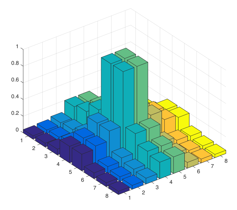
(a) Normalized spatial spectrum for $8$x$8$ MIMO channel

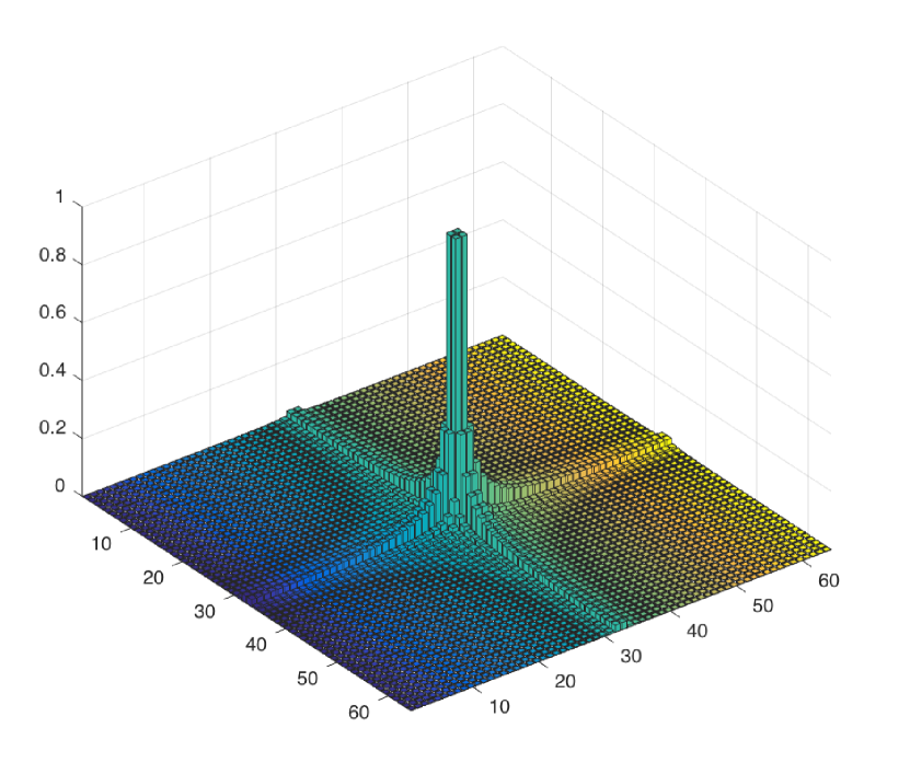
(b) Normalized spatial spectrum for $64$x$64$ MIMO channel

Figure 4: Normalized spatial spectrum for $8$x$8$ and $64$x$64$ MIMO channels.

The spatial spectrum $|\underline{{\mathbf{G}}}|$ (the $\hat{}$ accent is removed for notational convenience) is directly used in weighted sparse signal recovery. The structured random codebook design, however, requires the indices of the dominant sub-6 $\text{\,}\mathrm{GHz}$ AoA and AoD directions. The indices of the dominant direction can be found as

$$\{\underline{i}^{\star},\underline{j}^{\star}\}=\underset{1\leq\underline{i}\leq\underline{M}_{{\mathrm{R}}{\mathrm{X}}},1\leq\underline{j}\leq\underline{M}_{{\mathrm{T}}{\mathrm{X}}}}{\arg\max}|[{\mathbf{G}}]_{\underline{i},\underline{j}}|.$$ (15)

IV-B2 Second stage (OOB-aided compressed beam-selection)

We explain the OOB-aided compressed beam-selection in three parts. The first part is the weighted sparse recovery using information from a single subcarrier, the second is the structured random codebook design, and the third is the joint weighted sparse recovery using information from all active subcarriers.

Weighted sparse recovery: The OMP based sparse recovery assumes that the prior probability of the support is uniform, i.e., all elements of the unknown can be active with the same probability $p$. If some prior information about the non-uniformity in the support is available, the OMP algorithm can be modified to incorporate this prior information. In [22] a modified OMP algorithm called logit weighted - OMP (LW-OMP) was proposed for non-uniform prior probabilities. Assume that ${\mathbf{p}}\in{\mathbb{R}}^{M_{{\mathrm{T}}{\mathrm{X}}}M_{{\mathrm{R}}{\mathrm{X}}}}$ is the vector of prior probabilities. Specifically, the $r$th element of $\boldsymbol{\mathsf{g}}[k]$ can be active with prior probability $0\leq[{\mathbf{p}}]_{r}\leq 1$. Then $r^{\star}$ can be found using LW-OMP as

$$r^{\star}=\underset{1\leq r\leq M_{{\mathrm{R}}{\mathrm{X}}}M_{{\mathrm{T}}{\mathrm{X}}}}{\arg\max}|[\boldsymbol{\Psi}]_{:,r}^{\ast}\boldsymbol{\mathsf{y}}[k]|+w([{\mathbf{p}}]_{r}),$$ (16)

where $w([{\mathbf{p}}]_{r})$ is an additive weighting function. The authors refer the interested reader to [22] for the details of LW-OMP and the selection of $w([{\mathbf{p}}]_{r})$. The general form of $w([{\mathbf{p}}]_{r})$ can be given as $w([{\mathbf{p}}]_{r})=J_{{\mathrm{w}}}\log\dfrac{[{\mathbf{p}}]_{r}}{1-[{\mathbf{p}}]_{r}}$, where $J_{{\mathrm{w}}}$ is a constant that depends on sparsity level, the amplitude of the unknown coefficients, and the noise level. In the absence of prior information, (16) can be solved using uniform probability ${\mathbf{p}}=\delta{\mathbf{1}}$, where $0<\delta<=1$, which is equivalent to solving (13).

The spatial information from sub-6 $\text{\,}\mathrm{GHz}$ can be used to obtain a proxy for ${\mathbf{p}}$. The probability vector ${\mathbf{p}}\in{\mathbb{R}}^{M_{{\mathrm{R}}{\mathrm{X}}}M_{{\mathrm{T}}{\mathrm{X}}}}$ is obtained using $|\underline{{\mathbf{G}}}|\in{\mathbb{R}}^{\underline{M}_{{\mathrm{R}}{\mathrm{X}}}\times\underline{M}_{{\mathrm{T}}{\mathrm{X}}}}$. To obtain ${\mathbf{p}}$, we remove the dimensional discrepancy and find a scaled spatial spectrum $|\underline{{\mathbf{G}}}_{\mathrm{s}}|=g_{{\mathrm{s}}}(|\underline{{\mathbf{G}}}|)$, where $g_{{\mathrm{s}}}(\cdot):{\mathbb{R}}^{\underline{M}_{{\mathrm{R}}{\mathrm{X}}}\times\underline{M}_{{\mathrm{T}}{\mathrm{X}}}}\rightarrow{\mathbb{R}}^{M_{{\mathrm{R}}{\mathrm{X}}}\times M_{{\mathrm{T}}{\mathrm{X}}}}$ is a two-dimensional scaling function. As an example, the scaling function can be implemented using bi-cubic interpolation [51]. The scaled spatial spectrum $|\underline{{\mathbf{G}}}_{\mathrm{s}}|$ corresponding to Fig. 4(a) is shown in Figure 5. A simple proxy of the probability vector based on the scaled spectrum $|\underline{{\mathbf{G}}}_{s}|$ can be

$${\mathbf{p}}=J_{{\mathrm{p}}}\dfrac{|\underline{{\mathbf{g}}}_{\mathrm{s}}-\min(\underline{{\mathbf{g}}}_{\mathrm{s}})|}{\max(\underline{{\mathbf{g}}}_{\mathrm{s}}-\min(\underline{{\mathbf{g}}}_{\mathrm{s}}))},$$ (17)

where $J_{\mathrm{p}}$ is an appropriately chosen constant and $\underline{{\mathbf{g}}}_{\mathrm{s}}={\rm vec}(\underline{{\mathbf{G}}}_{\mathrm{s}})$. Initially the minimum of the spectrum $\underline{{\mathbf{g}}}_{\mathrm{s}}$ is subtracted to ensure all entries are non-negative. Then the spectrum is normalized to meet the probability constraint $0\leq[{\mathbf{p}}]_{r}\leq 1$. The scaling constant $J_{\mathbf{p}}\in(0,1]$ captures the reliability of the OOB-information. The reliability is a function of the sub-6 $\text{\,}\mathrm{GHz}$ and mmWave spatial congruence, and operating SNR. For highly reliable information, a higher value can be used for $J_{\mathrm{p}}$.

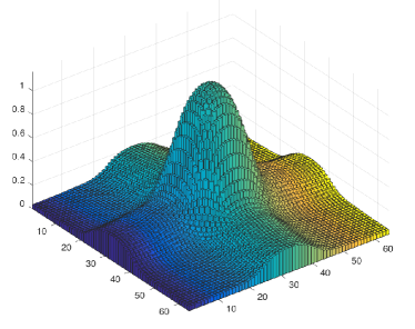
Figure 5: The $64$x$64$ scaled spatial spectrum of the $8$x$8$ spatial spectrum in Fig. 4(a).

Structured random codebooks: So far we have considered random codebooks that respect the analog hardware constraints, i.e., constant modulus and quantized phase-shifts. The random codebooks used for training, however, can be tailored to OOB information. We describe the design of structured codebooks for precoders, but it also applies to the combiners.

Note that the beamspace representation of the channel divides the spatial AoD range into $\underline{M}_{{\mathrm{T}}{\mathrm{X}}}$ intervals of width $\frac{1}{\underline{M}_{{\mathrm{T}}{\mathrm{X}}}}$ each. We call these intervals angle bins. Recall from (15) that $\underline{j}^{\star}$ is the index associated with the dominant AoD. Thus, the interval $[\underline{\omega}_{\underline{j}^{\star}}-\frac{1}{2\underline{M}_{{\mathrm{T}}{\mathrm{X}}}},\underline{\omega}_{\underline{j}^{\star}}+\frac{1}{2\underline{M}_{{\mathrm{T}}{\mathrm{X}}}})$ is the estimated dominant sub-6 $\text{\,}\mathrm{GHz}$ spatial angle bin. Due to a large number of antennas at mmWave in comparison with sub-6 $\text{\,}\mathrm{GHz}$, the mmWave anlge bins have a smaller width, and several mmWave angle bins fall in one sub-6 $\text{\,}\mathrm{GHz}$ angle bin. We create a set $\mathcal{J}$ using the mmWave angle bins that fall in the interval $[\underline{\omega}_{\underline{j}^{\star}}-\frac{1}{2\underline{M}_{{\mathrm{T}}{\mathrm{X}}}},\underline{\omega}_{\underline{j}^{\star}}+\frac{1}{2\underline{M}_{{\mathrm{T}}{\mathrm{X}}}})$, i.e., $\mathcal{J}=\{\phi_{j}:\phi_{j}=\arcsin(\frac{\omega_{j}}{d}),\omega_{j}\in[\underline{\omega}_{\underline{j}^{\star}}-\frac{1}{2\underline{M}_{{\mathrm{T}}{\mathrm{X}}}},\underline{\omega}_{\underline{j}^{\star}}+\frac{1}{2\underline{M}_{{\mathrm{T}}{\mathrm{X}}}}),j\in[M_{{\mathrm{T}}{\mathrm{X}}}]\}$. Using the set $\mathcal{J}$, we obtain a deterministic codebook ${\mathbf{D}}={\mathbf{a}}_{{\mathrm{T}}{\mathrm{X}}}(\mathcal{J})$, where ${\mathbf{a}}_{{\mathrm{T}}{\mathrm{X}}}(\mathcal{J})$ is the array response vector ${\mathbf{a}}_{{\mathrm{T}}{\mathrm{X}}}$ evaluated at the elements of $\mathcal{J}$. Next, we construct a super-codebook $\bar{\mathbf{F}}$ containing $\bar{N}_{{\mathrm{T}}{\mathrm{X}}}$ codewords according to [47]. The desired codebook then consists of the $N_{{\mathrm{T}}{\mathrm{X}}}$ codewords from the super codebook that have the highest correlation with the deterministic codebook ${\mathbf{D}}$. The procedure to generate structured precoding codebooks is summarized in Algorithm 2. The LW-OMP algorithm with structured codebooks is referred to as structured LW-OMP.

Algorithm 2 Structured random codebook design

1:$\underline{j}^{\star}$

2:${\mathbf{F}}$

3:Construct a deterministic codebook ${\mathbf{D}}={\mathbf{a}}_{{\mathrm{T}}{\mathrm{X}}}(\mathcal{J})$, where $\mathcal{J}=\{\phi_{j}:\phi_{j}=\arcsin(\frac{\omega_{j}}{d}),\omega_{j}\in[\underline{\omega}_{\underline{j}^{\star}}-\frac{1}{2\underline{M}_{{\mathrm{T}}{\mathrm{X}}}},\underline{\omega}_{\underline{j}^{\star}}+\frac{1}{2\underline{M}_{{\mathrm{T}}{\mathrm{X}}}}),j\in[M_{{\mathrm{T}}{\mathrm{X}}}]\}$.

4:Construct a super-codebook $\bar{\mathbf{F}}$ using $\bar{N}_{{\mathrm{T}}{\mathrm{X}}}$ random codewords generated according to [47].

5:Let ${\mathbf{N}}=\bar{\mathbf{F}}^{\ast}{\mathbf{D}}$. Populate the index set $\mathcal{M}$ with the indices of $N_{{\mathrm{T}}{\mathrm{X}}}$ rows of ${\mathbf{N}}$ that have the largest 2-norms.

6:Create the precoding matrix ${\mathbf{F}}=[\bar{\mathbf{F}}]_{:,\mathcal{M}}$.

Joint weighted sparse recovery: If the unknowns $\boldsymbol{\mathsf{g}}[k]$ were recovered on all subcarriers, a suitable criterion for choosing $r^{\star}$ could be $r^{\star}=\underset{1\leq r\leq M_{{\mathrm{R}}{\mathrm{X}}}M_{{\mathrm{T}}{\mathrm{X}}}}{\arg\max}\sum_{k\in[K]}|[\boldsymbol{\mathsf{g}}[k]]_{r}|$. One can recover the vectors $\boldsymbol{\mathsf{g}}[k]\leavevmode\nobreak\ \forall k\in K$ individually on each subcarrier and then find $r^{\star}$. Instead, we note that the unknown sparse vectors have a similar sparsity pattern i.e., they share an approximately common support [52]. To exploit the common support property, we formulate the problem of recovering $\boldsymbol{\mathsf{g}}[k]\leavevmode\nobreak\ \forall k\in K$ jointly using measurements from all subcarriers. Formally, we collect all vectors $\boldsymbol{\mathsf{y}}[k]\leavevmode\nobreak\ \forall k\in[K]$ in a matrix $\bar{\boldsymbol{\mathsf{Y}}}$, which can be written as

$$\bar{\boldsymbol{\mathsf{Y}}} =\left[\boldsymbol{\mathsf{y}}[1]\leavevmode\nobreak\ \boldsymbol{\mathsf{y}}[2]\leavevmode\nobreak\ \cdots\leavevmode\nobreak\ \boldsymbol{\mathsf{y}}[K]\right],$$

$$=\boldsymbol{\Psi}\left[\boldsymbol{\mathsf{g}}[1]\leavevmode\nobreak\ \boldsymbol{\mathsf{g}}[2]\leavevmode\nobreak\ \cdots\leavevmode\nobreak\ \boldsymbol{\mathsf{g}}[K]\right]+[\boldsymbol{\mathsf{v}}[1]\leavevmode\nobreak\ \boldsymbol{\mathsf{v}}[2]\leavevmode\nobreak\ \cdots\leavevmode\nobreak\ \boldsymbol{\mathsf{v}}[K]],$$

$$=\boldsymbol{\Psi}\bar{\boldsymbol{\mathsf{G}}}+\bar{\boldsymbol{\mathsf{V}}}.$$ (18)

The columns of $\bar{\boldsymbol{\mathsf{G}}}$ are approximately jointly sparse, i.e., $\bar{\boldsymbol{\mathsf{G}}}$ has only a few non-zero rows. The sparse recovery problems of the form (18) are referred to as MMV problems. The simultaneous OMP (SOMP) algorithm [23] is an OMP variant tailored for MMV problems. Using SOMP, $r^{\star}$ can be found as

$$r^{\star}=\underset{1\leq r\leq M_{{\mathrm{R}}{\mathrm{X}}}M_{{\mathrm{T}}{\mathrm{X}}}}{\arg\max}\sum_{k\in[K]}|[\boldsymbol{\Psi}]_{:,r}^{\ast}\boldsymbol{\mathsf{y}}[k]|.$$ (19)

The OOB information can be incorporated in SOMP algorithm via logit weighting and structured codebooks. Specifically, the logit weighted - SOMP (LW-SOMP) algorithm [53] finds $r^{\star}$ by

$$r^{\star}=\underset{1\leq r\leq M_{{\mathrm{R}}{\mathrm{X}}}M_{{\mathrm{T}}{\mathrm{X}}}}{\arg\max}\sum_{k\in[K]}|[\boldsymbol{\Psi}]_{:,r}^{\ast}\boldsymbol{\mathsf{y}}[k]|+w([{\mathbf{p}}]_{r}).$$ (20)

The LW-SOMP algorithm used with structured random codebooks is termed structured LW-SOMP.

V Simulation Results

In this section, we present simulation results to test the performance of the proposed OOB-aided mmWave beam-selection strategies. The sub-6 $\text{\,}\mathrm{GHz}$ system operates at $\underline{f}=3.5\leavevmode\nobreak\ $\text{\,}\mathrm{GHz}$$ with $1\leavevmode\nobreak\ $\text{\,}\mathrm{MHz}$$ bandwidth and $\underline{M}_{{\mathrm{R}}{\mathrm{X}}}=\underline{M}_{{\mathrm{T}}{\mathrm{X}}}=4$ antennas. The mmWave system operates at $f=28\leavevmode\nobreak\ $\text{\,}\mathrm{GHz}$$ with $320\leavevmode\nobreak\ $\text{\,}\mathrm{MHz}$$ bandwidth and $M_{{\mathrm{R}}{\mathrm{X}}}=M_{{\mathrm{T}}{\mathrm{X}}}=32$ antennas. Both systems use ULAs with half wavelength spacing $\underline{d}=d=1/2$. The number of OFDM subcarriers is $K=256$, and the CP length is $L_{{\mathrm{c}}}=K/4=64$. With the chosen operating frequencies, the number of antennas, and the inter-element spacing, the array aperture for sub-6 $\text{\,}\mathrm{GHz}$ and mmWave arrays is the same. Further, as $K+L_{{\mathrm{c}}}=320$, the chosen sub-6 $\text{\,}\mathrm{GHz}$ and mmWave bandwidths imply that the mmWave OFDM block has the same time duration as the sub-6 $\text{\,}\mathrm{GHz}$ symbol. The transmission power for sub-6 $\text{\,}\mathrm{GHz}$ and mmWave systems is $\underline{P}_{{\mathrm{t}}}=P_{{\mathrm{t}}}=37\leavevmode\nobreak\ $\text{\,}\mathrm{dB}${\mathrm{m}}$, and the path-loss coefficient at sub-6 $\text{\,}\mathrm{GHz}$ and mmWave is $3$. The sub-6 $\text{\,}\mathrm{GHz}$ channel is frequency flat, whereas the mmWave channel is frequency selective with $L=63$ taps. The number of quantization bits for analog phase-shifters are $D_{{\mathrm{R}}{\mathrm{X}}}=D_{{\mathrm{T}}{\mathrm{X}}}=\log_{2}(32)=5$ to realize the DFT codebooks. The raised cosine filter with a roll off factor of $1$ is used as a pulse shaping filter.

To study the performance of OOB-aided compressed beam-selection, we fix the channel parameters of sub-6 $\text{\,}\mathrm{GHz}$ and mmWave in the first experiment. The performance of OOB-aided beam-selection with varying degrees of spatial congruence between sub-6 $\text{\,}\mathrm{GHz}$ and mmWave is studied in the second experiment. The sub-6 $\text{\,}\mathrm{GHz}$ and mmWave channels have $\underline{C}=4$ and $C=3$ clusters respectively, each contributing $\underline{R}_{\mathrm{c}}=R_{\mathrm{c}}=10$ rays. We assume that the clusters are distributed uniformly in time and space. Hence, $\underline{\tau}_{\underline{c}}\sim U[0,\underline{\tau}_{\max}]$ and $\tau_{c}\sim U[0,\tau_{\max}]$. As the maximum delay spread of sub-6 $\text{\,}\mathrm{GHz}$ channel is expected to be larger than the maximum delay spread of mmWave [35, 36, 37, 38], we choose $\underline{\tau}_{\max}\approx 57\leavevmode\nobreak\ $\text{\,}\mathrm{ns}$$ and $\tau_{\max}\approx 48\leavevmode\nobreak\ $\text{\,}\mathrm{ns}$$ i.e., approximately $20\%$ larger maximum delay spread for sub-6 $\text{\,}\mathrm{GHz}$. The mean AoAs/AoDs of the clusters are distributed as $\{\underline{\theta}_{c},\underline{\phi}_{c}\}\sim U[-\frac{\pi}{2},\frac{\pi}{2})$ and $\{\theta_{c},\phi_{c}\}\sim U[-\frac{\pi}{2},\frac{\pi}{2})$. The relative time delays of the paths within the clusters are drawn from zero mean uniform distributions with RMS AS $\underline{\sigma}_{\underline{\tau}_{r_{\underline{c}}}}=\frac{\underline{\tau}_{\max}}{20\sqrt{12}}$ and $\sigma_{\tau_{r_{c}}}=\frac{\tau_{\max}}{20\sqrt{12}}$. The relative AoA/AoD shifts come from zero mean uniform distributions with AS $\{\underline{\sigma}_{\underline{\vartheta}_{\underline{c}}},\underline{\sigma}_{\underline{\varphi}_{\underline{c}}}\}=2.4^{\circ}\approx$0.042\text{\,}\mathrm{rad}$$ and $\{\sigma_{\vartheta_{c}},\sigma_{\varphi_{c}}\}=2^{\circ}\approx$0.035\text{\,}\mathrm{rad}$$. We use the replacement and perturbation models described in Section II with the angle modifier adjusted to limit the angles in $[-\frac{\pi}{2},\frac{\pi}{2})$.

The metric used for performance comparison is the effective achievable rate $R_{\rm{eff}}$ defined as

$$R_{\rm{eff}}=\dfrac{\eta}{EK}\sum_{e=1}^{E}\sum_{k=1}^{K}\log_{2}\left(1+\frac{P_{{\mathrm{t}}}}{K\sigma_{\check{\boldsymbol{\mathsf{v}}}}^{2}}|{\mathbf{a}}_{{\mathrm{R}}{\mathrm{X}}}^{\ast}(\nu_{\hat{i}})\boldsymbol{\mathsf{H}}[k]{\mathbf{a}}_{{\mathrm{T}}{\mathrm{X}}}(\omega_{\hat{j}})|^{2}\right),$$ (21)

where $\{\hat{i},\hat{j}\}$ are the estimated transmit and receive codeword indices, $E$ is the number of independent trials for ensemble averaging, $\eta\triangleq\max(0,1-\frac{N_{{\mathrm{R}}{\mathrm{X}}}\times N_{{\mathrm{T}}{\mathrm{X}}}}{T_{{\mathrm{c}}}})$, and $T_{{\mathrm{c}}}$ is the channel coherence time in OFDM blocks. With the channel coherence of $T_{{\mathrm{c}}}$ blocks and a training of $N_{{\mathrm{R}}{\mathrm{X}}}\times N_{{\mathrm{T}}{\mathrm{X}}}$ blocks, $1-\frac{N_{{\mathrm{R}}{\mathrm{X}}}\times N_{{\mathrm{T}}{\mathrm{X}}}}{T_{{\mathrm{c}}}}$ is the fraction of time/blocks that are used for data transmission. Thus, $\eta$ captures the loss in achievable rate due to the training.

V-A OOB-aided compressed beam-selection

In this experiment, we test the performance of OOB-aided compressed beam-selection in comparison with in-band only compressed beam-selection. The TX-RX separation for this experiment is fixed at $40\text{\,}\mathrm{m}$. The compressed beam-selection is performed using information on a single subcarrier, chosen uniformly at random from the $K$ subcarriers. The number of independent trials is $E=2000$. The number of measurements for exhaustive-search are fixed at $32\times 32=1024$. The rate results as a function of the number of measurements $N_{{\mathrm{R}}{\mathrm{X}}}\times N_{{\mathrm{T}}{\mathrm{X}}}$ are shown in Fig. 6. It can be observed that throughout the range of interest the OOB-aided compressed beam-selection using LW-OMP has a better effective rate in comparison with OMP. Further structured LW-OMP improves on the performance of LW-OMP, validating the benefit of using structured random codebooks.

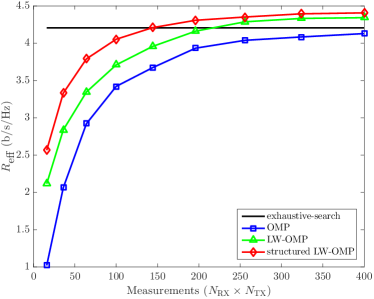
Figure 6: Effective rate of the structured LW-OMP approach versus the number of measurements $N_{{\mathrm{R}}{\mathrm{X}}}\times N_{{\mathrm{T}}{\mathrm{X}}}$ with $40\text{\,}\mathrm{m}$ TX-RX separation and $T_{{\mathrm{c}}}=6(M_{{\mathrm{R}}{\mathrm{X}}}\times M_{{\mathrm{T}}{\mathrm{X}}})=6144$ blocks.

It is observed from Fig. 6 that the effective rate of structured LW-OMP only slightly improves on the rate of exhaustive-search. This, however, is true for large channel coherence $T_{{\mathrm{c}}}$ values. We plot the effective rate of the proposed structured LW-OMP based compressed beam-selection for three channel coherence values in Fig. 7. As the coherence time of the channel decreases, the advantage of the proposed approach becomes significant. As an example, for a medium channel coherence time i.e., $4(M_{{\mathrm{R}}{\mathrm{X}}}\times M_{{\mathrm{T}}{\mathrm{X}}})$, the proposed structured LW-OMP based compressed beam-selection can reduce the training overhead of exhaustive-search by over $20$x and the overhead of LW-OMP by $4$x. The gains for smaller channel coherence times are more pronounced. Therefore, the proposed approach is suitable for applications with rapidly varying channels e.g., V2X communications.

To study the fraction of times the proposed approach recovers the best beam-pair, we define and evaluate the success percentage of the proposed approach. The success percentage is defined as

$$\mathrm{SP}=\dfrac{1}{E}\sum_{e=1}^{E}|\hat{r}^{\star}\cap\mathcal{B}_{N}|,$$ (22)

where $\hat{r}^{\star}$ is the index estimated by the proposed approach and $\mathcal{B}_{N}$ is the set containing the actual indices corresponding to the $N$ best TX/RX beam-pairs. When $N=1$, the set $\mathcal{B}_{1}$ has only one element and that is the index corresponding to the beam-pair with the highest receive power. For $N>1$, the set has $N$ entries that are indices corresponding to the $N$ beam-pairs with the highest receive power. Using a set of indices, instead of the index corresponding to the best beam-pair, generalizes the study and reveals an interesting behavior about selecting one of the better beam-pairs in comparison with selecting the best beam-pair. For now, note that due to grid offset and the presence of multiple clusters in the mmWave channel, it is possible that the proposed approach does not recover the best beam-pair and still manages to provide a decent effective rate. We populate the set $\mathcal{B}_{N}$ by performing exhaustive-search in a noiseless channel. We do so as the exhaustive-search in a noisy channel is itself subject to errors. This behavior is revealed in Fig. 8, where the exhaustive-search succeeds $\approx 74\%$ of the times for $\mathcal{B}_{1}$ and $\approx 80\%$ of the times for $\mathcal{B}_{5}$. The success percentage of the proposed structured LW-OMP algorithm is $\approx 50\%$ for $\mathcal{B}_{1}$ and $\approx 75\%$ for $\mathcal{B}_{5}$. The high success percentage for $\mathcal{B}_{5}$ is a ramification of having several strong candidate beam-pairs due to grid offset and the presence of multiple clusters. Note that even though the proposed approach has a (slightly) inferior success percentage for $\mathcal{B}_{5}$ compared with the exhaustive-search, the training overhead of the proposed approach is significantly lower. With the overhead factored in, the proposed approach is advantageous compared to exhaustive-search as evidenced by the effective rate results in Fig. 7.

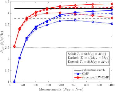
Figure 7: Effective rate of the structured LW-OMP approach versus the number of measurements $N_{{\mathrm{R}}{\mathrm{X}}}\times N_{{\mathrm{T}}{\mathrm{X}}}$ with $40\text{\,}\mathrm{m}$ TX-RX separation and three different channel coherence times $T_{{\mathrm{c}}}$.

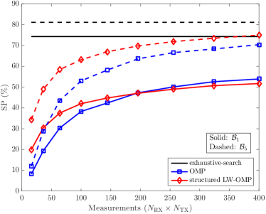
Figure 8: Success percentage of the structured LW-OMP approach versus the number of measurements $N_{{\mathrm{R}}{\mathrm{X}}}\times N_{{\mathrm{T}}{\mathrm{X}}}$ with $40\text{\,}\mathrm{m}$ TX-RX separation.

Next, we evaluate the performance of structured LW-SOMP based compressed beam-selection using information from all active subcarriers. The TX-RX separation is $80\text{\,}\mathrm{m}$, and with this separation the pre-beamforming per subcarrier SNR is $\approx$-10\text{\,}\mathrm{dB}$$. The results of this experiment are shown in Fig. 9. The structured LW-SOMP achieves a better effective rate in comparison with LW-SOMP. Due to the use of training information from all subcarriers, both structured LW-SOMP and LW-SOMP reach the effective rate of exhaustive-search with a handful of measurements. For low channel coherence times $T_{{\mathrm{c}}}$, the compressed beam-selection approaches, especially OOB-aided compressed beam-selection, will outperform exhaustive-search.

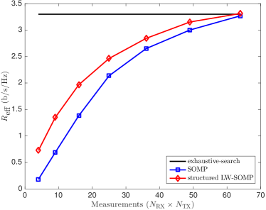
Figure 9: Effective rate of the structured LW-SOMP approach versus the number of measurements $N_{{\mathrm{R}}{\mathrm{X}}}\times N_{{\mathrm{T}}{\mathrm{X}}}$ with $80\text{\,}\mathrm{m}$ TX-RX separation and $T_{{\mathrm{c}}}=6(M_{{\mathrm{R}}{\mathrm{X}}}\times M_{{\mathrm{T}}{\mathrm{X}}})=6144$ blocks.

V-B Impact of mismatch in spatial parameters

The performance of OOB-aided approaches is a function of the congruence between sub-6 $\text{\,}\mathrm{GHz}$ and mmWave channels. We choose structured LW-OMP as a representative OOB-aided beam-selection approach and test the effective rate of structured LW-OMP with varying degrees of congruence between sub-6 $\text{\,}\mathrm{GHz}$ and mmWave. It is worth highlighting that in the proposed OOB-aided beam-selection strategies only spatial information of the sub-6 $\text{\,}\mathrm{GHz}$ channels is used. As such mismatch in the time parameters of sub-6 $\text{\,}\mathrm{GHz}$ and mmWave is not expected to impact the performance of OOB-aided approaches. Hence, we test the performance of structured LW-OMP as a function of mismatch in the spatial parameters. Specifically, we assume a single cluster in sub-6 $\text{\,}\mathrm{GHz}$ and mmWave i.e., $\underline{C}=1$ and $C=1$ and study the impact of mismatch in the AoA/AoD and AS of the sub-6 $\text{\,}\mathrm{GHz}$ and mmWave clusters. The channel parameters not explicitly mentioned in this experiment are consistent with the previously used setup. For this experiment, the number of measurements is $N_{{\mathrm{T}}{\mathrm{X}}}\times N_{{\mathrm{R}}{\mathrm{X}}}=64$, the coherence time is $T_{{\mathrm{c}}}=\infty$, and the number of independent trials is $E=5000$.

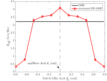
Figure 10: Effective rate of the structured LW-OMP approach versus sub-6 $\text{\,}\mathrm{GHz}$ AoA with $200\text{\,}\mathrm{m}$ TX-RX separation.

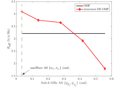
Figure 11: Effective rate of the structured LW-OMP approach versus sub-6 $\text{\,}\mathrm{GHz}$ AS with $200\text{\,}\mathrm{m}$ TX-RX separation.

We study the impact of mismatch between the mean AoA/AoD of the sub-6 $\text{\,}\mathrm{GHz}$ and mmWave cluster in Fig. 10. We keep the mean AoA/AoD of the mmWave cluster fixed at $\{\theta_{c},\phi_{c}\}=\{0,0\}$\text{\,}\mathrm{rad}$$. We also keep the mean AoD of sub-6 $\text{\,}\mathrm{GHz}$ fixed at $\underline{\phi}_{\underline{c}}=$0\text{\,}\mathrm{rad}$$ and vary the mean AoA $\underline{\theta}_{\underline{c}}$. Expectedly when the $\underline{\theta}_{\underline{c}}$ matches $\theta_{c}$, we see the highest rate for structured LW-OMP. As $\underline{\theta}_{\underline{c}}$ differs from $\theta_{c}$ by more than $\approx$0.5\text{\,}\mathrm{rad}$$, the structured LW-OMP becomes inferior to in-band only OMP based beam-selection. Keeping the AoA $\underline{\theta}_{\underline{c}}$ fixed and varying the AoD $\underline{\phi}_{\underline{c}}$ is expected to yield similar results.

We also study the impact of mismatch between the AS of the sub-6 $\text{\,}\mathrm{GHz}$ and mmWave cluster. We keep the AoA/AoD of sub-6 $\text{\,}\mathrm{GHz}$ and mmWave fixed at $\{\underline{\theta}_{\underline{c}},\underline{\phi}_{\underline{c}}\}=\{0,0\}$\text{\,}\mathrm{rad}$$ and $\{\theta_{c},\phi_{c}\}=\{0,0\}$\text{\,}\mathrm{rad}$$. The relative AoA/AoD shifts of the paths within mmWave cluster have zero mean, uniform distribution and AS $\{\sigma_{\vartheta_{c}},\sigma_{\varphi_{c}}\}=2^{\circ}\approx$0.035\text{\,}\mathrm{rad}$$. The relative AoA/AoD shifts of the paths within sub-6 $\text{\,}\mathrm{GHz}$ cluster are also zero man and uniformly distributed. We test the performance of the structured LW-OMP algorithm for varying AS of the sub-6 $\text{\,}\mathrm{GHz}$ cluster. Specifically, we increase the AS of sub-6 $\text{\,}\mathrm{GHz}$ cluster compared to mmWave, which is in accordance with the observations of prior work [38, 36]. Both the AoA and AoD AS are increased equally. The effective rate is plotted in Fig. 11. As expected, the gain of structured LW-OMP decreases as the AS of sub-6 $\text{\,}\mathrm{GHz}$ increases. In this particular experiment, when the AS of sub-6 $\text{\,}\mathrm{GHz}$ was $\approx$0.368\text{\,}\mathrm{rad}$$, i.e., $\approx 10.5$x the mmWave AS, the performance of structured LW-OMP became inferior to the in-band only OMP.

VI Conclusion

In this paper, we used the sub-6 $\text{\,}\mathrm{GHz}$ spatial information to reduce the training overhead of beam-selection in an analog mmWave system. We formulated the compressed beam-selection problem as a weighted sparse recovery problem with structured random codebooks to incorporate out-of-band information. We evaluated the achievable rate of the proposed out-of-band aided beam-selection strategies using multi-band frequency dependent channels. The channels were generated using the proposed multi-band channel generation methodology that is consistent with the frequency dependent channel behavior observed in the prior work. From the rate results, it was concluded that the training overhead of in-band only compressed beam-selection can be reduced by $4$x if the out-of-band information is used.

There are several directions for future work. The frequency dependent channel estimation strategy can be calibrated with the emerging joint channel modeling results for sub-6 $\text{\,}\mathrm{GHz}$ and mmWave. The out-of-band aided beam-selection strategies can be explored for arrays other than uniform linear arrays, e.g., circular and planar arrays. Finally, using out-of-band information in hybrid analog/digital and fully digital low-resolution architectures for mmWave systems is an interesting direction for future work.

References

- [1] A. Ali and R. W. Heath Jr., “Compressed beam-selection in millimeter wave systems with out-of-band partial support information,” in Proc. IEEE Int. Conf. Acoust., Speech Signal Process. (ICASSP), Mar. 2017.
- [2] Z. Pi and F. Khan, “An introduction to millimeter-wave mobile broadband systems,” IEEE Commun. Mag., vol. 49, no. 6, pp. 101–107, Jun. 2011.
- [3] T. S. Rappaport et al., “Millimeter wave mobile communications for 5G cellular: It will work!” IEEE Access, vol. 1, pp. 335–349, May 2013.
- [4] A. Alkhateeb et al., “Channel estimation and hybrid precoding for millimeter wave cellular systems,” IEEE J. Sel. Topics Signal Process., vol. 8, no. 5, pp. 831–846, Oct. 2014.
- [5] J. Choi, “Beam selection in mm-Wave multiuser MIMO systems using compressive sensing,” IEEE Trans. Commun., vol. 63, no. 8, pp. 2936–2947, Aug. 2015.
- [6] J. Seo et al., “Training beam sequence design for millimeter-wave MIMO systems: A POMDP framework,” IEEE Trans. Signal Process., vol. 64, no. 5, pp. 1228–1242, Mar. 2016.
- [7] J. Wang, “Beam codebook based beamforming protocol for multi-Gbps millimeter-wave WPAN systems,” IEEE J. Sel. Areas Commun., vol. 27, no. 8, pp. 1390–1399, Oct. 2009.
- [8] S. Hur et al., “Millimeter wave beamforming for wireless backhaul and access in small cell networks,” IEEE Trans. Commun., vol. 61, no. 10, pp. 4391–4403, Oct. 2013.
- [9] Y. Kishiyama et al., “Future steps of LTE-A: Evolution toward integration of local area and wide area systems,” IEEE Wireless Commun., vol. 20, no. 1, pp. 12–18, Feb. 2013.
- [10] R. C. Daniels and R. W. Heath Jr., “Multi-band modulation, coding, and medium access control,” IEEE 802.11-07/2780R1, pp. 1–18, Nov. 2007.
- [11] M. Peter et al., “Measurement campaigns and initial channel models for preferred suitable frequency ranges,” Millimetre-Wave Based Mobile Radio Access Network for Fifth Generation Integrated Communications, Tech. Rep., Mar. 2016.
- [12] T. Nitsche et al., “Steering with eyes closed: mm-wave beam steering without in-band measurement,” in Proc. IEEE Int. Conf. Comput. Commun. (INFOCOM), Apr. 2015, pp. 2416–2424.
- [13] A. D. Angelica. (2013) Google’s self-driving car gathers nearly 1gb/sec. [Online]. Available: http://www.kurzweilai.net/ googles- self- driving- car- gathers- nearly- 1- gbsec
- [14] Y. J. Li, “An overview of the DSRC/WAVE technology,” in Proc. Qual., Rel., Security Robustness Heterogeneous Netw. Springer, Nov. 2010, pp. 544–558.
- [15] M. Rumney et al., LTE and the evolution to 4G wireless: Design and measurement challenges. John Wiley & Sons, 2013.
- [16] J. Choi et al., “Millimeter wave vehicular communication to support massive automotive sensing,” IEEE Commun. Mag., vol. 54, no. 12, pp. 160–167, Dec. 2016.
- [17] V. Va, J. Choi, and R. W. Heath Jr, “The impact of beamwidth on temporal channel variation in vehicular channels and its implications,” IEEE Trans. Veh. Technol., early access.
- [18] J. G. Andrews et al., “What will 5G be?” IEEE J. Sel. Areas Commun., vol. 32, no. 6, pp. 1065–1082, Jun. 2014.
- [19] T. Bai and R. W. Heath Jr., “Coverage and rate analysis for millimeter-wave cellular networks,” IEEE Trans. Wireless Commun., vol. 14, no. 2, pp. 1100–1114, Feb. 2015.
- [20] S. Singh et al., “Tractable model for rate in self-backhauled millimeter wave cellular networks,” IEEE J. Sel. Areas Commun., vol. 33, no. 10, pp. 2196–2211, Oct. 2015.
- [21] “Federal communications commission. Spectrum frontiers R&0 and FNPRM: FCC16-89.” Jul. 2016.
- [22] J. Scarlett, J. S. Evans, and S. Dey, “Compressed sensing with prior information: Information-theoretic limits and practical decoders,” IEEE Trans. Signal Process., vol. 61, no. 2, pp. 427–439, Jan 2013.
- [23] J. A. Tropp, A. C. Gilbert, and M. J. Strauss, “Simultaneous sparse approximation via greedy pursuit,” in Proc. IEEE Int. Conf. Acoust., Speech Signal Process. (ICASSP), vol. 5, Mar. 2005, pp. 721–724.
- [24] T. Asté et al., “Downlink beamforming avoiding DOA estimation for cellular mobile communications,” in Proc. IEEE Int. Conf. Acoust., Speech Signal Process. (ICASSP), May 1998, pp. 3313–3316.
- [25] K. Hugl, K. Kalliola, and J. Laurila, “Spatial reciprocity of uplink and downlink radio channels in FDD systems,” May, COST 273 Technical Document TD(02) 066, 2002.
- [26] M. Jordan, X. Gong, and G. Ascheid, “Conversion of the spatio-temporal correlation from uplink to downlink in FDD systems,” in Proc. IEEE Wireless Commun. Netw. Conf. (WCNC), Apr. 2009, pp. 1–6.
- [27] A. Decurninge, M. Guillaud, and D. T. Slock, “Channel covariance estimation in massive MIMO frequency division duplex systems,” in Proc. IEEE Glob. Telecom. Conf. (GLOBECOM), Dec. 2015, pp. 1–6.
- [28] D. Vasisht et al., “Eliminating channel feedback in next-generation cellular networks,” in Proc. ACM SIGCOMM, Aug. 2016, pp. 398–411.
- [29] J. Shen et al., “Compressed CSI acquisition in FDD massive MIMO: How much training is needed?” IEEE Trans. Wireless Commun., vol. 15, no. 6, pp. 4145–4156, Jun. 2016.
- [30] A. Ali, N. González-Prelcic, and R. W. Heath Jr., “Estimating millimeter wave channels using out-of-band measurements,” in Proc. Inf. Theory Appl. (ITA) Wksp, Feb. 2016, pp. 1–5.
- [31] N. González-Prelcic, R. Méndez-Rial, and R. W. Heath Jr., “Radar aided beam alignment in mmwave V2I communications supporting antenna diversity,” in Proc. Inf. Theory Appl. (ITA) Wksp, Feb. 2016, pp. 1–5.
- [32] M. K. Samimi and T. S. Rappaport, “3-D millimeter-wave statistical channel model for 5G wireless system design,” IEEE Trans. Microw. Theory Techn., vol. 64, no. 7, pp. 2207–2225, Jul. 2016.
- [33] ITU, “Propagation data and prediction methods for the planning of indoor radiocommunication systems and radio local area networks in the frequency range 900 MHz to 100 GHz,” ITU-R Recommendations, Tech. Rep., 2001.
- [34] E. J. Violette et al., “Millimeter-wave propagation at street level in an urban environment,” IEEE Trans. Geosci. Remote Sens., vol. 26, no. 3, pp. 368–380, May 1988.
- [35] R. J. Weiler et al., “Simultaneous millimeter-wave multi-band channel sounding in an urban access scenario,” in Proc. Eur. Conf. Antennas Propag. (EuCAP), Apr. 2015, pp. 1–5.
- [36] A. S. Poon and M. Ho, “Indoor multiple-antenna channel characterization from 2 to 8 GHz,” in Proc. IEEE Int. Conf. Commun. (ICC), May 2003, pp. 3519–3523.
- [37] S. Jaeckel et al., “5G channel models in mm-wave frequency bands,” in Proc. Eur. Wireless Conf. (EW), May 2016, pp. 1–6.
- [38] A. Ö. Kaya, D. Calin, and H. Viswanathan. (2016, Apr.) 28 GHz and 3.5 GHz wireless channels: Fading, delay and angular dispersion.
- [39] R. C. Qiu and I.-T. Lu, “Multipath resolving with frequency dependence for wide-band wireless channel modeling,” IEEE Trans. Veh. Technol., vol. 48, no. 1, pp. 273–285, Jan. 1999.
- [40] K. Haneda, A. Richter, and A. F. Molisch, “Modeling the frequency dependence of ultra-wideband spatio-temporal indoor radio channels,” IEEE Trans. Antennas Propag., vol. 60, no. 6, pp. 2940–2950, Jun. 2012.
- [41] D. Dupleich et al., “Simultaneous multi-band channel sounding at mm-Wave frequencies,” in Proc. Eur. Conf. Antennas Propag. (EuCAP), Apr. 2016, pp. 1–5.
- [42] P. Ky et al., “Frequency dependency of channel parameters in urban LOS scenario for mmwave communications,” in Proc. Eur. Conf. Antennas Propag. (EuCAP), Apr. 2016, pp. 1–5.
- [43] K. Haneda, J.-i. Takada, and T. Kobayashi, “Experimental investigation of frequency dependence in spatio-temporal propagation behaviour,” in Proc. Eur. Conf. Antennas Propag. (EuCAP), Nov. 2007, pp. 1–6.
- [44] V. Nurmela et al., “METIS channel models,” Mobile and wireless communications enablers for the twenty-twenty information society, Tech. Rep., Feb. 2015.
- [45] A. M. Sayeed, “Deconstructing multiantenna fading channels,” IEEE Trans. Signal Process., vol. 50, no. 10, pp. 2563–2579, Oct. 2002.
- [46] P. Schniter and A. Sayeed, “Channel estimation and precoder design for millimeter-wave communications: The sparse way,” in Proc. Asilomar Conf. Signals, Syst. Comput. (ASILOMAR), Nov. 2014, pp. 273–277.
- [47] A. Alkhateeb, G. Leus, and R. W. Heath Jr., “Compressed sensing based multi-user millimeter wave systems: How many measurements are needed?” in Proc. IEEE Int. Conf. Acoust., Speech Signal Process. (ICASSP), Apr. 2015, pp. 2909–2913.
- [48] J. A. Tropp and A. C. Gilbert, “Signal recovery from random measurements via orthogonal matching pursuit,” IEEE Trans. Inf. Theory, vol. 53, no. 12, pp. 4655–4666, Dec 2007.
- [49] M. L. Bencheikh, Y. Wang, and H. He, “Polynomial root finding technique for joint DOA DOD estimation in bistatic MIMO radar,” Signal Process., vol. 90, no. 9, pp. 2723–2730, Sep. 2010.
- [50] M. Bengtsson and B. Ottersten, “Low-complexity estimators for distributed sources,” IEEE Trans. Signal Process., vol. 48, no. 8, pp. 2185–2194, Aug. 2000.
- [51] R. Keys, “Cubic convolution interpolation for digital image processing,” IEEE Trans. Acoust., Speech, Signal Process., vol. 29, no. 6, pp. 1153–1160, Dec. 1981.
- [52] Z. Gao et al., “Spatially common sparsity based adaptive channel estimation and feedback for FDD massive MIMO,” IEEE Trans. Signal Process., vol. 63, no. 23, pp. 6169–6183, Dec. 2015.
- [53] Z. Li et al., “Compressed sensing reconstruction algorithms with prior information: logit weight simultaneous orthogonal matching pursuit,” in Proc. IEEE Veh. Tech. Conf. (VTC), May 2014, pp. 1–5.