Abstract

We consider the differential equation that Zernike proposed to classify aberrations of wavefronts in a circular pupil, whose value at the boundary can be nonzero. On this account the quantum Zernike system, where that differential equation is seen as a Schrödinger equation with a potential, is special in that it has a potential and boundary condition that are not standard in quantum mechanics. We project the disk on a half-sphere and there we find that, in addition to polar coordinates, this system separates in two additional coordinate systems (non-orthogonal on the pupil disk), which lead to Schrödinger-type equations with Pöschl-Teller potentials, whose eigen-solutions involve Legendre, Gegenbauer and Jacobi polynomials. This provides new expressions for separated polynomial solutions of the original Zernike system that are real. The operators which provide the separation constants are found to participate in a superintegrable cubic Higgs algebra.

1 Introduction: the Zernike operator

The differential operator and eigenvalue equation of Zernike [20] are

$$\hat{Z}^{(\alpha,\beta)}\Psi{{\scriptstyle(}{\bf r}{\scriptstyle)}}:=\Big{(}\nabla^{2}+\alpha({\bf r}\cdot\nabla)^{2}+\beta\,{\bf r}\cdot\nabla\Big{)}\Psi{{\scriptstyle(}{\bf r}{\scriptstyle)}}=-E\,\Psi{{\scriptstyle(}{\bf r}{\scriptstyle)}},$$ (1)

for real parameters $\alpha$ and $\beta$. In order to describe the shape of scalar optical wavefields constrained by a unit circular exit pupil, and such that at its boundary ${{\scriptstyle|}{\bf r}{\scriptstyle|}}=1$ the wavefields have constant absolute value $c=|\Psi{{\scriptstyle(}{\bf r}{\scriptstyle)}}|_{{{\scriptscriptstyle|}{\bf r}{\scriptscriptstyle|}}=1}$, Zernike found that for the two-dimensional case, the operator (1) can be self-adjoint under the inner product over the pupil disk, only when the two parameters have the values $\alpha_{\scriptscriptstyle\rm Z}=-1$ and $\beta_{\scriptscriptstyle\rm Z}=-2$, as we show in Sect. 2.

This system and its solutions have many important properties which have been analyzed thoroughly in several optical and mathematical papers [2, 3, 15, 11, 19, 18, 8]. Yet it seems that the symmetries obtained when this system is projected from the disk on the half-sphere, have not been yet elucidated up to now.

The Zernike differential equation (1) can evidently be separated and solved in polar coordinates $(r,\phi)$. As was shown in Ref. [17], the classical counterpart of this equation describes a system which is separable in polar and elliptic coordinates plus, when projected on the manifold of a sphere or hyperboloid, displays separability in other three and six orthogonal coordinate systems respectively. In Sect. 3 we solve the separated polar and radial equations, the former yielding circular harmonics, and the latter hypergeometric polynomials that match those of Zernike [20]. The quest for higher symmetries starts in Sect. 4, where we map the disk on a half-sphere with coinciding boundaries. This step is crucial because it allows the orthogonal coordinates on the sphere to map onto non-orthogonal coordinates on the disk, where the Zernike equation also separates, and where the separation constants provide extra integrals of motion.

In Section 5 we introduce three coordinate systems on the sphere, whose $\vartheta=0$ poles point along the $z$-, $x$- and $y$-axes. The first returns essentially the solutions of the previous sections, while the other two yield solutions in terms of products of a Legendre and a Gegenbauer polynomial. In Section 6 the operators that provide the separation constants are organized through their commutators into the nonlinear cubic Higgs superintegrable algebra [7, 10]. The concluding Sect. 7 recapitulates the construction and adds some further remarks on Zernike-type systems.

2 Boundary conditions and restrictions

As we mentioned in the Introduction, the Hilbert space of square-integrable functions $f{{\scriptstyle(}{\bf r}{\scriptstyle)}}\in{\cal L}^{2}({\cal D})$, on the unit disk ${\cal D}:=\{{{\scriptstyle|}{\bf r}{\scriptstyle|}}\leq 1\}$ is determined by the inner product

$$(f,g)_{\cal D}:=\int_{\cal D}{\rm d}^{2}{\bf r}\,f{{\scriptstyle(}{\bf r}{\scriptstyle)}}^{*}g{{\scriptstyle(}{\bf r}{\scriptstyle)}}=\int_{0}^{1}\!r\,{\rm d}r\int_{-\pi}^{\pi}\!{\rm d}\phi\,f(r,\phi)^{*}g(r,\phi),$$ (2)

where the asterisk indicates complex conjugation, and where the functions are required to satisfy the boundary value $|f(1,\phi)|={}$constant. In this space, the Zernike operator (1) is required to be self-adjoint, namely,

$$(f,\hat{Z}^{(\alpha,\beta)}g)_{\cal D}=(\hat{Z}^{(\alpha,\beta)}f,g)_{\cal D}.$$ (3)

Written out in polar coordinates and separated in three summands, this operator is

$$\hat{Z}^{(\alpha,\beta)}=\hat{Z}_{2}^{(\alpha)}+\hat{Z}_{1}^{(\alpha,\beta)}+\hat{Z}_{\phi},$$ (4)

where

$$\hat{Z}_{2}^{(\alpha)}:=(1+\alpha r^{2})\partial^{2}_{r},\quad\hat{Z}_{1}^{(\alpha,\beta)}:=\bigg{(}\frac{1}{r}+(\alpha+\beta)r\bigg{)}\partial_{r},\quad\hat{Z}_{\phi}:=\frac{1}{r^{2}}\partial^{2}_{\phi}.$$ (5)

On each summand the integral (2) will be performed by parts yielding boundary terms. The last term we can immediately integrate by parts over $\phi$, yielding

$$(f,\hat{Z}_{\phi}g)_{\cal D}=(\hat{Z}_{\phi}f,g)_{\cal D}+\int_{0}^{1}\frac{{\rm d}r}{r}\bigg{(}(f^{*}\partial_{\phi}g-g\partial_{\phi}f^{*})\Big{|}_{\phi=-\pi}^{\pi}\bigg{)}.$$ (6)

The last term will evidently vanish when the functions are single-valued over the disk, so we can consider

$$f(r,\phi)=f_{m}{{\scriptstyle(}r{\scriptstyle)}}\frac{e^{{\rm i}m\phi}}{\sqrt{2\pi}},$$ (7)

with any integer $m$. Let us continue indicating by $f{{\scriptstyle(}r{\scriptstyle)}},\,g{{\scriptstyle(}r{\scriptstyle)}}$, functions of the radius $r$ alone, suppressing their index $m$, and obviating the integral over $\phi$ in (2) that will yield unity.

The first-order differential term $\hat{Z}_{1}^{(\alpha,\beta)}$ in (5) will be now integrated by parts over $r|_{0}^{1}$, giving a left-over integral and a boundary term,

$$(f,\hat{Z}_{1}g)_{r}=-(\hat{Z}_{1}f,g)_{r}-2(\alpha+\beta)\!\int_{0}^{1}\!r\,{\rm d}r\,f^{*}g+\Big{(}1+(\alpha+\beta)r^{2}\Big{)}f^{*}g\Big{|}_{0}^{1}.$$ (8)

Proceeding similarly with the second-order differential term $\hat{Z}_{2}^{(\alpha)}$, we obtain

$$\begin{array}[]{rcl}(f,\hat{Z}_{2}g)_{r}&=&\displaystyle(\hat{Z}_{2}f,g)_{r}+\int_{0}^{1}\!{\rm d}r\,\Big{(}2(1+3\alpha r^{2})(\partial_{r}f^{*})g+6\alpha rf^{*}g\Big{)}\\ &&\displaystyle{}+\bigg{(}r(1+\alpha r^{2})\Big{(}f^{*}\partial_{r}g-(\partial_{r}f^{*})g\Big{)}-(1+3\alpha r^{2})f^{*}g\bigg{)}\bigg{|}_{0}^{1}.\end{array}$$ (9)

Summing (8) and (9) yields

$$\begin{array}[]{l}\Big{(}f,(\hat{Z}_{2}{+}\hat{Z}_{1})g\Big{)}_{\!r}=\Big{(}(\hat{Z}_{2}{-}\hat{Z}_{1})f,g\Big{)}_{\!r}\\ \displaystyle{\quad}+2\int_{0}^{1}\!r\,{\rm d}r\,\Big{(}(2\alpha-\beta)f^{*}g+(1/r+3\alpha r)(\partial_{r}f^{*})g\Big{)}\\ \displaystyle{\quad}+\bigg{(}r(1+\alpha r^{2})\Big{(}f^{*}\partial_{r}g-(\partial_{r}f^{*})g\Big{)}+r^{2}(\beta-2\alpha)f^{*}g\bigg{)}\bigg{|}_{0}^{1}.\end{array}$$ (10)

The boundary term is zero at $r=0$; for $r=1$ and generally nonzero values for $f(1)$, $g(1)$ or their derivatives, the first summand vanishes when $\alpha=-1$, and then the coefficient of second summand will also vanish when $\beta=2\alpha=-2$; for these values of $\alpha$ and $\beta$, the remaining integral term in the right-hand side of (10) will then be $2\int_{0}^{1}r\,{\rm d}r\,(1/r-3r)(\partial_{r}f^{*})g=2(\hat{Z}_{1}^{(-1,-2)}f,g)_{r}$, as can be seen from (5). The last term $\hat{Z}_{\phi}$ in (6) is independently self-adjoint, so it follows that the Zernike operator $\hat{Z}^{(-1,-2)}$ satisfies the required self-adjointness condition (3).

Given the form of the angular part of the Zernike differential operator $\hat{Z}_{\phi}$ in (5), its eigenfunctions being $\sim e^{{\rm i}m\phi}$ for all integers $m\in\{0,\pm 1,\pm 2,\ldots\}$, we may separate the solutions $\Psi{{\scriptstyle(}{\bf r}{\scriptstyle)}}$ of (1) as

$$\Psi(r,\phi):=R^{{\scriptscriptstyle(}m{\scriptscriptstyle)}}{{\scriptstyle(}r{\scriptstyle)}}\frac{e^{{\rm i}m\phi}}{\sqrt{2\pi}},$$ (11)

turning the Zernike equation (1) into an ordinary differential equation for the radial factor $R^{{\scriptscriptstyle(}m{\scriptscriptstyle)}}{{\scriptstyle(}r{\scriptstyle)}}$,

$$r^{2}(1-r^{2})\frac{{\rm d}^{2}R^{{\scriptscriptstyle(}m{\scriptscriptstyle)}}{{\scriptstyle(}r{\scriptstyle)}}}{{\rm d}r^{2}}+r(1-3r^{2})\frac{{\rm d}R^{{\scriptscriptstyle(}m{\scriptscriptstyle)}}{{\scriptstyle(}r{\scriptstyle)}}}{{\rm d}r}-m^{2}R^{{\scriptscriptstyle(}m{\scriptscriptstyle)}}{{\scriptstyle(}r{\scriptstyle)}}=-Er^{2}\,R^{{\scriptscriptstyle(}m{\scriptscriptstyle)}}{{\scriptstyle(}r{\scriptstyle)}},$$ (12)

where the values of $E$ will be determined by the square-integrable solutions that can be normalized as $R^{{\scriptscriptstyle(}m{\scriptscriptstyle)}}(1)={}$constant.

3 The Zernike basis of functions on the disk

The radial differential equation of Zernike (12) is of hypergeometric type. Writing $R^{{\scriptscriptstyle(}m{\scriptscriptstyle)}}{{\scriptstyle(}r{\scriptstyle)}}=r^{m}F(r^{2})$, the factor $F{{\scriptstyle(}z{\scriptstyle)}}$ is solution of the hypergeometric equation [5, Eq. 9.151],

$$z(1{-}z)F^{\prime\prime}+\Big{(}(m{+}1)-(m{+}2)z\Big{)}F^{\prime}-{\textstyle\frac{1}{4}}\Big{(}m(m{+}2)-E\Big{)}F=0,$$ (13)

which has one solution of the form ${}_{2}F_{\!1}(a,b;c;z)$, with parameters

$$a={\textstyle\frac{1}{2}}(m{+}1)\pm{\textstyle\frac{1}{2}}\sqrt{E{+}1},\quad b={\textstyle\frac{1}{2}}(m{+}1)\mp{\textstyle\frac{1}{2}}\sqrt{E{+}1},\quad c=m+1.$$ (14)

Since $m$ is integer and $c$ must be positive, the absolute value ${{\scriptstyle|}m{\scriptstyle|}}$ should be understood for $\surd m^{2}$ in (12). Also, since $c=a+b$, the solution will be logarithmically singular at $z=r^{2}=1$ unless the hypergeometric series terminates and is a polynomial. This occurs when we write $E:=n(n+2)$ and ask $n-{{\scriptstyle|}m{\scriptstyle|}}$ to be an even non-negative integer, thus defining the radial quantum number

$$n_{r}:={\textstyle\frac{1}{2}}(n-{{\scriptstyle|}m{\scriptstyle|}})\in\{0,1,2,\ldots\},$$ (15)

and the energy $E$ in (1) is then given by the principal quantum number $n$,

$$E=n(n+2),\quad n=2n_{r}+{{\scriptstyle|}m{\scriptstyle|}}\in\{0,1,2,\ldots\}.$$ (16)

Hence, the square integrable solutions to the radial Zernike equation (12) in the interval $r\in[0,1]$ are of the form

$$R_{n}^{m}(r) := A_{n,m}\,r^{{{\scriptscriptstyle|}m{\scriptscriptstyle|}}}\,{}_{2}F_{\!1}(-n_{r},\,n_{r}+{{\scriptstyle|}m{\scriptstyle|}}+1;\ {{\scriptstyle|}m{\scriptstyle|}}+1;\,r^{2})$$ (17)

$$= A_{n,m}\,\bigg{(}{n_{r}+{{\scriptstyle|}m{\scriptstyle|}}\atop{{\scriptstyle|}m{\scriptstyle|}}}\bigg{)}^{-1}r^{{{\scriptscriptstyle|}m{\scriptscriptstyle|}}}P^{({{\scriptscriptstyle|}m{\scriptscriptstyle|}},0)}_{n_{r}}(1{-}2r^{2}),$$ (18)

where $A_{n,m}$ is a constant and we recognize the identity of the hypergeometric with Jacobi polynomials of degree $n_{r}$ in $(1-2r^{2})$ [5, Eq. 8.962.1].

Zernike’s original requirement [20, Eq. (22)] was that $R_{n}^{m}(1)=1$, leading to choose the constant $A_{n,m}$ in (17)–(18) given by a sign and binomial coefficient, so that $A^{\scriptscriptstyle\rm Zernike}_{n,m}:=(-1)^{n_{r}}\Big{(}{n_{r}+{{\scriptscriptstyle|}m{\scriptscriptstyle|}}\atop{{\scriptscriptstyle|}m{\scriptscriptstyle|}}}\Big{)}$ defines his disk polynomials as

$$Z^{m}_{n}(r,\phi):=R^{m}_{n}(r)\,\bigg{\{}\begin{array}[]{rl}\cos m\phi,&\hbox{for }m\geq 0,\\ \sin m\phi,&\hbox{for }m<0.\end{array}$$ (19)

In the present paper we prefer to attend the ‘quantum-mechanical’ normalization of the disk functions, using the orthogonality of the Jacobi polynomials over $r\in[0,1]$ in the form [5, Eq. 7.391]

$$\int_{0}^{1}r\,{\rm d}r\,\Big{|}r^{{\scriptscriptstyle|}m{\scriptscriptstyle|}}P^{({{\scriptscriptstyle|}m{\scriptscriptstyle|}},0)}_{n_{r}}(1{-}2r^{2})\Big{|}^{2}=\frac{1}{2(n+1)}.$$ (20)

Since $\int_{-\pi}^{\pi}{\rm d}\phi=2\pi$, we adopt the normalization constant for the disk functions as $A_{n,m}=\sqrt{2(n{+}1)/2\pi}$ in (11), so they are

$$\Psi_{n}^{m}(r,\phi):=(-1)^{n_{r}}\sqrt{\frac{n+1}{\pi}}\,r^{{\scriptscriptstyle|}m{\scriptscriptstyle|}}P^{({{\scriptscriptstyle|}m{\scriptscriptstyle|}},0)}_{n_{r}}(1{-}2r^{2})\,e^{{\rm i}m\phi},$$ (21)

with $n=2n_{r}+{{\scriptstyle|}m{\scriptstyle|}}$. At the center of the disk $\Psi_{n}^{m}(0,\phi)=0$ for $m\neq 0$, while (for $n$ even) $\Psi_{n}^{0}(0,\phi)=\sqrt{(n{+}1)/\pi}$, and $\Psi_{0}^{0}(r,\phi)=1/\surd\pi$. At the circle boundary $r=1$,

$$\Psi_{n}^{m}(1,\phi)={\textstyle\frac{1}{8}}(n+{{\scriptstyle|}m{\scriptstyle|}})(n+{{\scriptstyle|}m{\scriptstyle|}}-2)\sqrt{\frac{n+1}{\pi}}\,e^{{\rm i}m\phi}.$$ (22)

These wavefunctions satisfy the orthonormality relation

$$(\Psi_{n}^{m},\Psi_{n^{\prime}}^{m^{\prime}})_{\cal D}=\int_{\cal D}{\rm d}^{2}{\bf r}\,\Psi_{n}^{m}{{\scriptstyle(}{\bf r}{\scriptstyle)}}^{*}\,\Psi_{n^{\prime}}^{m^{\prime}}{{\scriptstyle(}{\bf r}{\scriptstyle)}}=\delta_{n,n^{\prime}}\,\delta_{m,m^{\prime}},$$ (23)

and are solutions to the quantum Zernike Hamiltonian equation

$$-\hat{Z}\Psi_{n}^{m}{{\scriptstyle(}{\bf r}{\scriptstyle)}}:=\Big{(}{-\nabla}^{2}+({\bf r}\cdot\nabla)^{2}+2\,{\bf r}\cdot\nabla\Big{)}\Psi_{n}^{m}{{\scriptstyle(}{\bf r}{\scriptstyle)}}=n(n+2)\,\Psi_{n}^{m}{{\scriptstyle(}{\bf r}{\scriptstyle)}}.$$ (24)

Density plots of the Zernike disk polynomials are ubiquitous in the literature and on the web, so we need not reproduce here the real and imaginary parts of $\Psi_{n}^{m}(r,\phi)$ in (21). Below we shall display the new disk polynomials associated with separating coordinates different from the polar ones.

4 Finding additional constants of motion

For a fixed value of energy $E=n(n+2)$ given by the principal quantum number $n$ in (16), there is a range of radial and azimutal quantum numbers $n_{r}$ and $m$ that sum to $n=2n_{r}+{{\scriptstyle|}m{\scriptstyle|}}$. The degeneracy in $\pm m$ stems from the SO($2$) rotational symmetry of the disk $\cal D$ generated by the angular momentum operator

$$\hat{L}:=x\partial_{y}-y\partial_{x}.$$ (25)

But there is also a larger degeneracy between those two quantum numbers, present in the multiplets

$$m\in\{n,\,n-2,\,\ldots\,{-n}\},$$ (26)

that keep $n-m$ as even integers, and which indicates an SU($2$) symmetry and extra integrals of motion that we proceed to find. These must be of second degree in momentum, and would imply that other systems of separating coordinates exist. As is well known in two-dimensional flat space, the Helmholtz and Schrödinger equations allow separation of variables in four orthogonal systems, namely in Cartesian, polar, parabolic, and elliptic coordinates [14]. A simple analysis of the Zernike equation (1) on the unit disk $\cal D$ shows that only the polar system evinces this separation, so the question of existence of additional integrals of motion and of separating coordinates is open. Below we shall solve this problem by finding two integrals of the motion in addition to $\hat{L}$ in (25), which is the only obvious one.

Consider again the Zernike operator (1) with the values of $\alpha=-1$ and $\beta=-2$ that we saw in Sect. 2 to allow its self-adjointness on the unit disk $\cal D$, written in Cartesian coordinates,

$$\hat{Z}:=(1-x^{2})\partial_{xx}-2xy\partial_{xy}+(1-y^{2})\partial_{yy}-3(x\partial_{x}+y\partial_{y}).$$ (27)

Now we perform the similarity transformation

$$\widehat{W}:=A\hat{Z}A^{-1},\quad A{{\scriptstyle(}r{\scriptstyle)}}:=(1-x^{2}-y^{2})^{1/4}=(1-r^{2})^{1/4},$$ (28)

to obtain the new operator

$$\begin{array}[]{rcl}\widehat{W}&=&(1-x^{2})\partial_{xx}-2xy\partial_{xy}+(1-y^{2})\partial_{yy}-2(x\partial_{x}+y\partial_{y})\\[5.0pt] &&{}+{\textstyle\frac{1}{4}}(1-x^{2}-y^{2})^{-1}+{\textstyle\frac{3}{4}}.\end{array}$$ (29)

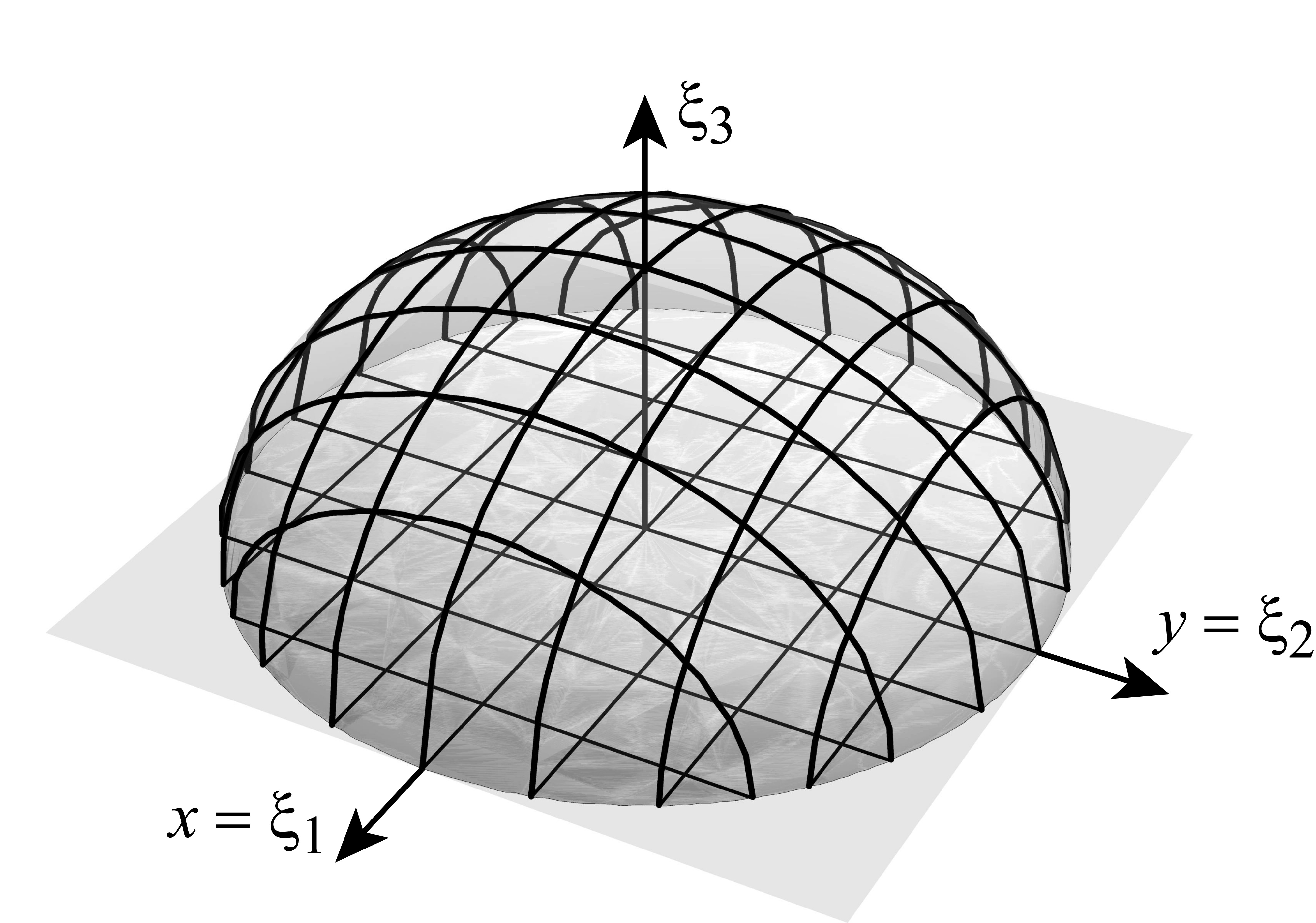
Figure 1: Map of the unit disk $\cal D$ on the unit upper hemisphere ${\cal H}_{+}$ through the orthogonal projection (30) of Cartesian coordinates.

As in the classical system [17], we shall map the unit disk $\cal D$ on the upper hemisphere ${\cal H}_{+}$, $\xi_{1}^{2}+\xi_{2}^{2}+\xi_{3}^{2}=1$, $\xi_{3}\geq 0$, embedded in a three-dimensional Euclidean space of coordinates $\{\xi_{i}\}_{i=1}^{3}$, using the orthogonal (or ‘vertical’) projection as shown in Fig. 1,

$$\xi_{1}=x,\quad\xi_{2}=y,\quad\xi_{3}=\sqrt{1-x^{2}-y^{2}},$$ (30)

where $\xi_{1}^{2}+\xi_{2}^{2}=r^{2}$, while the partial derivatives map on $\partial_{i}:=\partial/\partial\xi_{i}$ as

$$\partial_{x}=\partial_{1}-\frac{\xi_{1}}{\xi_{3}}\partial_{3},\qquad\partial_{y}=\partial_{2}-\frac{\xi_{2}}{\xi_{3}}\partial_{3}.$$ (31)

The second-order operator $\widehat{W}$ in (29), with $\partial_{ij}=\partial^{2}/\partial_{\xi_{i}}\partial_{\xi_{j}}$, thus becomes

$$\widehat{W} = (\xi_{2}^{2}+\xi_{3}^{2})\partial_{11}+(\xi_{1}^{2}+\xi_{3}^{2})\partial_{22}+(\xi_{1}^{2}+\xi_{2}^{2})\partial_{33}$$

$${}-2\xi_{1}\xi_{2}\partial_{12}-2\xi_{1}\xi_{3}\partial_{13}-2\xi_{2}\xi_{3}\partial_{23}-2\xi_{1}\partial_{1}-2\xi_{2}\partial_{2}-2\xi_{3}\partial_{3}$$

$${}+\frac{\xi_{1}^{2}+\xi_{2}^{2}}{4\xi_{3}^{2}}+1$$

$$= \Delta_{\scriptscriptstyle\rm LB}+\frac{\xi_{1}^{2}+\xi_{2}^{2}}{4\xi_{3}^{2}}+1,$$ (33)

where we have introduced the Laplace-Beltrami operator on the two-dimensional unit sphere

$$\Delta_{\scriptscriptstyle\rm LB}:=\hat{L}_{1}^{2}+\hat{L}_{2}^{2}+\hat{L}_{3}^{2},$$ (34)

and where $\{L_{i}\}_{i=1}^{3}$ are the generators of an SO($3$) Lie algebra,

$$\hat{L}_{1}:=\xi_{3}\partial_{2}-\xi_{2}\partial_{3},\quad\hat{L}_{2}:=\xi_{1}\partial_{3}-\xi_{3}\partial_{1},\quad\hat{L}_{3}:=\xi_{2}\partial_{1}-\xi_{1}\partial_{2}.$$ (35)

While the metric on the disk $\cal D$ is diagonal and distance is ${\rm d}s^{2}={\rm d}x^{2}+{\rm d}y^{2}$, the metric on the surface of the half-sphere ${\cal H}_{+}$ of $|\vec{\xi}\,|=1$, is

$${\bf g}=\left(\matrix{\displaystyle{1{+}\xi^{2}_{1}/\xi^{2}_{3}}&\displaystyle{\xi_{1}\xi_{2}/\xi^{2}_{3}}{}_{\mathstrut}\cr\displaystyle{\xi_{1}\xi_{2}/\xi^{2}_{3}}&\displaystyle{1{+}\xi^{2}_{2}/\xi^{2}_{3}}\cr}\right),\quad g:=\det{\bf g}=\frac{1}{\xi^{2}_{3}}=\frac{1}{1-(\xi^{2}_{1}{+}\xi^{2}_{2})},$$ (36)

so that distance is ${\rm d}s^{2}=\sum_{i,j=1}^{2}g_{i,j}{\rm d}\xi_{i}\,{\rm d}\xi_{j}$, and the surface elements on ${\cal H}_{+}$ and $\cal D$ are related by

$${\rm d}^{2}V(\vec{\xi}\,)=\sqrt{g}\,{\rm d}\xi_{1}\,{\rm d}\xi_{2}=\frac{{\rm d}\xi_{1}\,{\rm d}\xi_{2}}{\xi_{3}}=\frac{{\rm d}x\,{\rm d}y}{\sqrt{1-(x^{2}{+}y^{2})}}=\frac{{\rm d}^{2}{\bf r}}{\sqrt{1-r^{2}}}.$$ (37)

This clearly shows that the measure on ${\cal H}_{+}$ grows when $\xi_{3}\to 0$ ($r\to 1$) so that its vertical projection on the disk remains constant up to the boundary.

As a result, the quantum Zernike Hamiltonian equation (24) on the unit disk $\cal D$, written in terms of $\widehat{W}$, transforms to a quantum Schrödinger equation on the unit upper half-sphere ${\cal H}_{+}$ for wavefunctions $\Upsilon_{n}^{m}(\vec{\xi}\,)$ of the form

$$\Big{(}{-\Delta}_{\scriptscriptstyle\rm LB}-\omega^{2}\frac{\xi_{1}^{2}+\xi_{2}^{2}}{\xi_{3}^{2}}\Big{)}\Upsilon_{n}^{m}(\vec{\xi}\,)=(E+1)\Upsilon_{n}^{m}(\vec{\xi}\,),$$ (38)

which corresponds to a form of repulsive oscillator potential,

$$V_{\scriptscriptstyle\rm\!R}(\vec{\xi}\,):=-{\textstyle\frac{1}{2}}w^{2}\frac{\xi_{1}^{2}+\xi_{2}^{2}}{\xi_{3}^{2}}=-{\textstyle\frac{1}{2}}w^{2}\frac{r^{2}}{1-r^{2}},$$ (39)

that generalizes the superintegrable Higgs attractive oscillator [7, 6, 9], to a repusive one with negative coupling constant $-{\textstyle\frac{1}{2}}w^{2}$, whose wavefunctions are

$$\Upsilon_{n}^{m}(\vec{\xi}\,):=A{{\scriptstyle(}r{\scriptstyle)}}\,\Psi_{n}^{m}{{\scriptstyle(}{\bf r}{\scriptstyle)}}=(1-r^{2})^{1/4}\Psi_{n}^{m}(r,\phi)$$ (40)

where ${\bf r}$ is $(\xi_{1},\xi_{2})$ or $(r,\phi)$, and with energy eigenvalues

$${\cal E}:={\textstyle\frac{1}{2}}(E+1)={\textstyle\frac{1}{2}}(n+1)^{2},\quad n\in\{0,1,2,\ldots\}.$$ (41)

Because $A(1)=0$, the wavefunctions $\Upsilon_{n}^{m}(\vec{\xi}\,)$ in (40) vanish on the boundary $\xi_{3}=0$ of ${\cal H}_{+}$, while at the ‘top pole’ $\xi_{3}=1$, $r=0$, they have the values found for $\Psi_{n}^{m}{{\scriptstyle(}{\bf r}{\scriptstyle)}}$ after (21).

From the orthonormality relation between the wavefunctions $\Psi_{n}^{m}{{\scriptstyle(}{\bf r}{\scriptstyle)}}$ when integrated over the disk $\cal D$ in (23) for the inner product $(\circ,\circ)_{\cal D}$, under the proper inner product on the half-sphere ${\cal H}_{+}$ due to (37) and (40), the corresponding orthonormality of the wavefunctions $\Upsilon_{n}^{m}(\vec{\xi}\,)$ is

$$(\Upsilon_{n}^{m},\Upsilon_{n^{\prime}}^{m^{\prime}})_{{\cal H}_{+}}:=\int_{{\cal H}_{+}}{\rm d}^{2}V(\vec{\xi}\,)\,\Upsilon_{n}^{m}(\vec{\xi}\,)^{*}\,\Upsilon_{n^{\prime}}^{m^{\prime}}(\vec{\xi}\,)=(\Psi_{n}^{m},\Psi_{n^{\prime}}^{m^{\prime}})_{\cal D}=\delta_{n,n^{\prime}}\delta_{m,m^{\prime}}.$$ (42)

5 Solution to the Schrödinger equation (38)

The key to analyze the Zernike system in new light has been to map the unit disk $\cal D$ on the half-sphere ${\cal H}_{+}$. It is on this manifold that one can introduce in a natural way other coordinate systems. Indeed, the Higgs repulsive oscillator system (38) can be separated in four systems of coordinates: three mutually orthogonal spherical systems of coordinates [16], namely

System I: (43)

$$\hskip-30.0pt\xi_{1}=\sin\vartheta\cos\varphi,\quad\xi_{2}=\sin\vartheta\sin\varphi,\quad\xi_{3}=\cos\vartheta,\qquad\vartheta|_{0}^{\pi/2},\ \varphi|_{0}^{2\pi},$$

System II: (44)

$$\hskip-30.0pt\xi_{1}=\cos\vartheta^{\prime},\quad\xi_{2}=\sin\vartheta^{\prime}\cos\varphi^{\prime},\quad\xi_{3}=\sin\vartheta^{\prime}\sin\varphi^{\prime},\qquad\vartheta^{\prime}|_{0}^{\pi},\ \varphi^{\prime}|_{0}^{\pi},$$

System III: (45)

$$\hskip-30.0pt\xi_{1}=\sin\vartheta^{\prime\prime}\sin\varphi^{\prime\prime},\quad\xi_{2}=\cos\vartheta^{\prime\prime},\quad\xi_{3}=\sin\vartheta^{\prime\prime}\cos\varphi^{\prime\prime}.\qquad\vartheta^{\prime\prime}|_{0}^{\pi},\ \varphi^{\prime\prime}|_{-\pi/2}^{\pi/2},$$

and also the elliptic coordinate system.

Restricting our consideration in this paper only to the above three spherical systems, we now examine the form of the potential present in each. In Fig. 2 we show the three coordinate systems (43)–(45) on the sphere and on the projected disk, on which the solutions in this section will separate, and to appreciate that the latter two coordinate systems, while they are orthogonal over the sphere, they are non-orthogonal over the disk. Normally such coordinates are not considered when examining separability on a flat space.

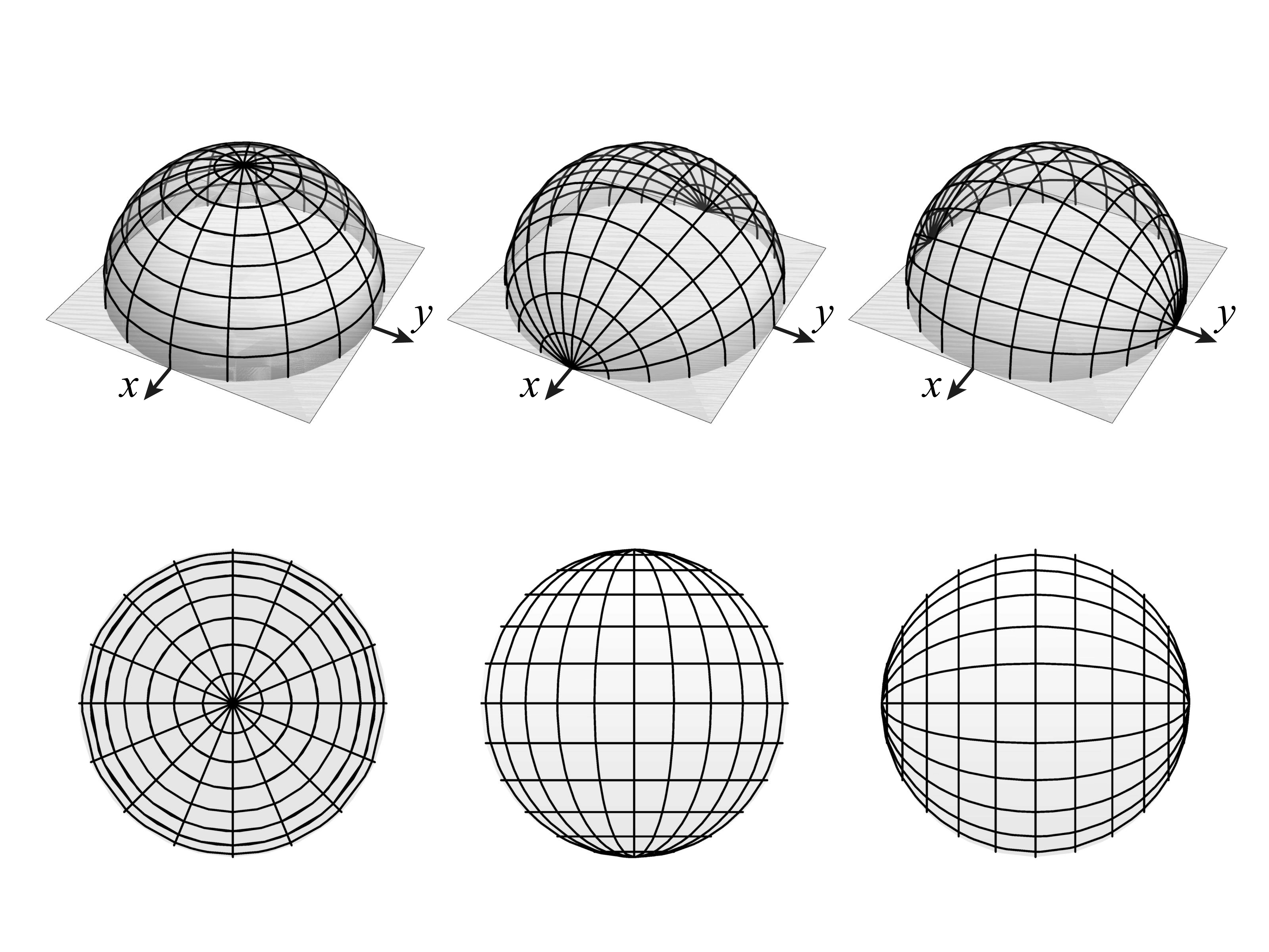
Figure 2: The coordinate systems (43)–(45). Top row: on the half-sphere ${\cal H}_{+}$, where the $\vartheta=0$ pole is directed along the vertical $z$-axis, and on the $x$- and $y$-axes. Bottom row: The same coordinate systems after projection over the disk $\cal D$.

5.1 The system I in (43)

In the spherical coordinate system $(\vartheta,\varphi)$ of (43) the repulsive oscillator potential (39) takes the form

$$V_{\scriptscriptstyle\rm\!R}(\vartheta)=-\frac{\xi_{1}^{2}+\xi_{2}^{2}}{8\xi_{3}^{2}}=-{\textstyle\frac{1}{8}}\tan^{2}\vartheta,$$ (46)

and the corresponding Schrödinger equation (38) has the form

$$\frac{1}{\sin\vartheta}\frac{\partial}{\partial\vartheta}\sin\vartheta\frac{\partial\Upsilon^{\scriptscriptstyle\rm I}(\vartheta,\varphi)}{\partial\vartheta}+\frac{1}{\sin^{2}\theta}\frac{\partial^{2}\Upsilon^{\scriptscriptstyle\rm I}(\vartheta,\varphi)}{\partial\varphi^{2}}+(2{\cal E}+{\textstyle\frac{1}{4}}\tan^{2}\vartheta)\Upsilon^{\scriptscriptstyle\rm I}(\vartheta,\varphi)=0.$$ (47)

We now separate the wave function according to the coordinates $(\vartheta,\varphi)$,

$$\Upsilon^{\scriptscriptstyle\rm I}(\vartheta,\varphi)=\frac{Z^{\scriptscriptstyle\rm I}(\vartheta)}{\sqrt{\sin\vartheta}}\,\frac{e^{{\rm i}m\varphi}}{\sqrt{2\pi}},\qquad m\in\{0,\pm 1,\pm 2,\ldots\},$$ (48)

so we come to find $Z^{\scriptscriptstyle\rm I}(\vartheta)$ as the solution of a ‘singular’ Pöschl-Teller-type equation,

$$\frac{{\rm d}^{2}Z^{\scriptscriptstyle\rm I}(\vartheta)}{{\rm d}\vartheta^{2}}+\bigg{(}2{\cal E}-\frac{m^{2}-\frac{1}{4}}{\sin^{2}\vartheta}+\frac{1}{4\cos^{2}\vartheta}\bigg{)}Z^{\scriptscriptstyle\rm I}(\vartheta)=0.$$ (49)

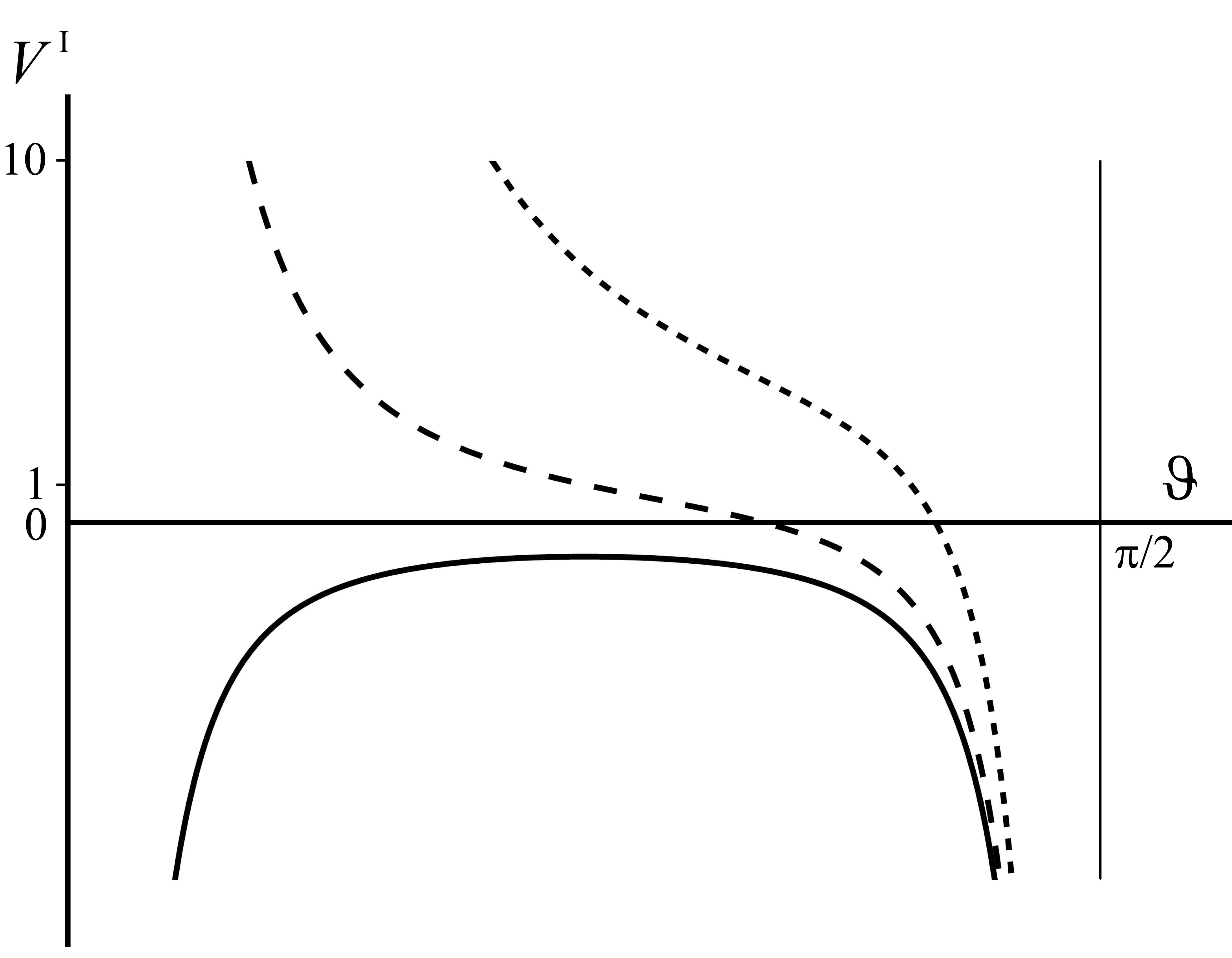
Figure 3: Effective potential $V_{\scriptscriptstyle\rm\!eff}^{\scriptscriptstyle\rm I}(\vartheta)=(m^{2}-1/4)/\sin^{2}\vartheta-1/4\cos^{2}\vartheta$ in (50), for $\vartheta\in(0,\pi/2)$ and values $m=0$ (continuous line), $m=1$ (dashed), and $m=2$ (dotted).

This equation describes the one-dimensional quantum wavefield in the effective potential

$$V_{\scriptscriptstyle\rm\!eff}^{\scriptscriptstyle\rm I}(\vartheta)=\frac{m^{2}-\frac{1}{4}}{\sin^{2}\vartheta}-\frac{1}{4\cos^{2}\vartheta},$$ (50)

shown in Fig. 3, which contains a strong repulsive singularity at $\vartheta=0$ (for $m\neq 0$) and a weak attractive singularity at $\vartheta={\textstyle\frac{1}{2}}\pi$, where we choose the self-adjoint extension with positive spectrum; when $m=0$ both singularities are weak and we follow the same choice. Such singularities of the Pöschl-Teller potentials have been considered in [4], and appear also in the coupling Clebsch-Gordan coefficients of two lower-bound ‘discrete’ representations of the Lorentz algebra so($2,1$) [1].

While in the general Pöschl-Teller potential (on a finite interval) one may have both positive and negative energies, we will have solutions of the Schrödinger equation whose potential (50) has only positive energy eigenvalues. Our task now is to find the square-integrable solutions of Eq. (49) that satisfy the boundary conditions of vanishing at the singularities $\vartheta=0$ and ${\textstyle\frac{1}{2}}\pi$ of (50),

$$Z^{\scriptscriptstyle\rm I}(0)=0,\qquad Z^{\scriptscriptstyle\rm I}({\textstyle\frac{1}{2}}\pi)=0,$$ (51)

with the additional requirement that at the boundary,

$$Z^{\scriptscriptstyle\rm I}(\vartheta)/\sqrt{\cos\vartheta}\Big{|}_{\vartheta=\pi/2}=\hbox{constant}\neq 0.$$ (52)

This requirement embodies the factor $A(r)=(1-r^{2})^{1/4}=\surd\cos\vartheta$ introduced in (28), and allows $\Upsilon^{\scriptscriptstyle\rm I}(\vartheta,\varphi)$ in (48) to be nonzero at the boundary $r=1$.

For the boundary conditions (51), the energy spectrum of ${\cal E}$ in (49) is positive and discrete, namely

$${\cal E}={\textstyle\frac{1}{2}}(n+1)^{2},\qquad n\in\{0,1,2,\ldots\},$$ (53)

as determined by $E$ in (16). To prove this proposition we replace in (49) the new variable $s:=\sin^{2}\vartheta$ and substitute

$$Z^{\scriptscriptstyle\rm I}(\vartheta)=s^{({{\scriptstyle|}m{\scriptstyle|}}+\frac{1}{2})/2}(1-s)^{1/4}f{{\scriptstyle(}s{\scriptstyle)}},$$ (54)

where $f{{\scriptstyle(}s{\scriptstyle)}}$ now satisfies

$$s(1-s)f^{{}^{\prime\prime}}+\Big{(}({{\scriptstyle|}m{\scriptstyle|}}+1)-s({{\scriptstyle|}m{\scriptstyle|}}+2)\Big{)}f^{{}^{\prime}}-{\textstyle\frac{1}{4}}\Big{(}({{\scriptstyle|}m{\scriptstyle|}}+1)^{2}-2{\cal E}\Big{)}f=0.$$ (55)

The solution of this equation that is regular at $s=0$ is a hypergeometric function,

$$f{{\scriptstyle(}s{\scriptstyle)}}=C\,{}_{2}F_{\!1}\Big{(}{\textstyle\frac{1}{2}}({{\scriptstyle|}m{\scriptstyle|}}{+}1+\sqrt{2{\cal E}}),\,{\textstyle\frac{1}{2}}({{\scriptstyle|}m{\scriptstyle|}}{+}1-\sqrt{2{\cal E}});{{\scriptstyle|}m{\scriptstyle|}}{+}1;s\Big{)},$$ (56)

where $C$ is a constant. The second solution to (55) diverges logarithmically at $s=0$, i.e., at $\vartheta=0$ and hence at the center of the disk $r=0$, so we disregard it.

Still, since the parameters of the hypergeometric function in (56) again sum as $a+b=c$, its behaviour at $s=1$ will also diverge logarithmically, as was the case in (14) for polar coordinates of the disk $\cal D$, and nevertheless the two boundary conditions in (51) are satisfied due to (54). To have solutions $\Upsilon^{\scriptscriptstyle\rm I}$ that can be a nonzero constant over the circle $r=1$ the third boundary condition (52) must hold, and again this requires the hypergeometric series to terminate as a polynomial. There is thus a subtle difference between quantization on the disk as performed in Sect. 3, and quantization on the half-sphere as done here. We must therefore demand that one of the two first parameters of the hypergeometric function in (56) be zero or a negative integer, which leads us to define again the radial quantum number

$$n_{r}:=-{\textstyle\frac{1}{2}}({{\scriptstyle|}m{\scriptstyle|}}+1-\sqrt{2{\cal E}})\in\{0,1,2,\ldots\},$$ (57)

as we did to find the spectrum in (16), thus proving the assertion in (53). We thus define the principal and radial quantum numbers related by the angular momentum parameter ${{\scriptstyle|}m{\scriptstyle|}}=\surd m^{2}$ in (48) and the Pöschl-Teller potential (50) by $n=2n_{r}+{{\scriptstyle|}m{\scriptstyle|}}$, and use them them to label the solutions in (49) as $Z^{\scriptscriptstyle\rm I}_{n_{r},m}(\vartheta)$. Using the boundary condition (52) to determine the appropriate constant $C$ in (56) we write thus the solution with the two quantum number labels as

$$Z^{\scriptscriptstyle\rm I}_{n_{r},m}(\vartheta) = \sqrt{2(n+1)}\frac{n_{r}!\,{{\scriptstyle|}m{\scriptstyle|}}!}{(n_{r}+{{\scriptstyle|}m{\scriptstyle|}})!}\,(\sin\vartheta)^{{{\scriptstyle|}m{\scriptstyle|}}+1/2}\,(\cos\vartheta)^{1/2}\,$$ (58)

$${}\times{}_{2}F_{\!1}(-n_{r},\,n_{r}+{{\scriptstyle|}m{\scriptstyle|}}+1;\,{{\scriptstyle|}m{\scriptstyle|}}+1;\sin^{2}\vartheta)$$

$$= \sqrt{2(n+1)}\,(\sin\vartheta)^{{{\scriptstyle|}m{\scriptstyle|}}+1/2}\,(\cos\vartheta)^{1/2}P_{n_{r}}^{({{\scriptstyle|}m{\scriptstyle|}},0)}(\cos 2\vartheta),$$ (59)

where again $P^{(\alpha,\beta)}_{n}(u)$ are the Jacobi polynomials, as was the case in the polar coordinate case (17). The wave functions $Z^{\scriptscriptstyle\rm I}_{n_{r}m}(\vartheta)$ in the interval $\vartheta\in[0,{\textstyle\frac{1}{2}}\pi]$ of ${\cal H}_{+}$ are normalized as

$$\int_{0}^{\pi/2}\!\!\!{\rm d}\vartheta\,Z^{\scriptscriptstyle\rm I}_{n_{r},m}(\vartheta)^{*}\,Z^{\scriptscriptstyle\rm I}_{n^{\prime}_{r},m}(\vartheta)=\delta_{n_{r},n^{\prime}_{r}},$$ (60)

which yields the orthonormalization for the $\Upsilon^{m}_{n}(\vartheta,\varphi)$ solution in (42).

Returning from the variables $(\vartheta,\varphi)$ of System I in (43) to the polar coordinates $(r,\phi)$, with $r=\sin\vartheta$ and $\phi=\varphi$, as shown in Fig. 2 (left), taking into account the connection between the functions $\Upsilon^{\scriptscriptstyle\rm I}(\vartheta,\phi)$ in (48) and $\Psi(r,\phi)$, and attaching the principal quantum number label, we obtain the result (21).

5.2 The system II in (44)

In the second spherical coordinate (44), the potential (39) expressed in the coordinates $(\vartheta^{\prime},\varphi^{\prime})$, is now

$$V^{\scriptscriptstyle\rm II}_{\scriptscriptstyle\rm\!eff}=-\frac{1}{8}\bigg{(}\frac{1}{\sin^{2}\vartheta^{\prime}\sin^{2}\varphi^{\prime}}-1\bigg{)}.$$ (61)

The corresponding quantum Zernike Hamiltonian equation (38) can be separated with the substitution

$$\Upsilon^{\scriptscriptstyle\rm II}(\vartheta^{\prime},\varphi^{\prime})=\frac{1}{\sqrt{\sin\vartheta^{\prime}}}S(\vartheta^{\prime})\,T(\varphi^{\prime}),$$ (62)

so we come to a system of two differential equations with a separation constant $k$,

$$\frac{{\rm d}^{2}S}{{\rm d}\vartheta^{{}^{\prime}2}}+\bigg{(}2{\cal E}-\frac{k^{2}-\frac{1}{4}}{\sin^{2}\vartheta^{\prime}}\bigg{)}S=0,\qquad\frac{{\rm d}^{2}T}{{\rm d}\varphi^{{}^{\prime}2}}+\bigg{(}k^{2}+\frac{1}{4\sin^{2}\varphi^{\prime}}\bigg{)}T=0.$$ (63)

These equations can be put in form where the Pöschl-Teller form is more evident introducing the new variables $\mu={\textstyle\frac{1}{2}}\varphi^{\prime}$ and $\nu={\textstyle\frac{1}{2}}\vartheta^{\prime}$, as

$$\frac{{\rm d}^{2}T(\mu)}{{\rm d}\mu^{2}}+\bigg{(}4k^{2}+\frac{1}{4\sin^{2}\mu}+\frac{1}{4\cos^{2}\mu}\bigg{)}T(\mu) = 0,$$ (64)

$$\frac{{\rm d}^{2}S(\nu)}{{\rm d}\nu^{2}}+\bigg{(}4{\cal E}^{2}+\frac{1-4k^{2}}{4\sin^{2}\nu}+\frac{1-4k^{2}}{4\cos^{2}\mu}\bigg{)}S(\nu) = 0.$$ (65)

The boundary condition at the weak singularities of (64) were discussed following Eq. (49), while those of (65) are even weaker due to the $-4k^{2}$ summand. Regarding the extra boundary condition analogue to (52) now is

$$T(\mu)/\surd\cos\mu\Big{|}_{\mu=\pi/2}=\hbox{constant}\neq 0.$$ (66)

Solving these equations we obtain the constant and the energies $\cal E$ in (53)

$$k=n_{1}+{\textstyle\frac{1}{2}},\quad{\cal E}={\textstyle\frac{1}{2}}(k+n_{2}+{\textstyle\frac{1}{2}})^{2}={\textstyle\frac{1}{2}}(n_{1}+n_{2}+1)^{2}={\textstyle\frac{1}{2}}(n+1)^{2}$$ (67)

where $n=n_{1}+n_{2}$ is the principal quantum number and $n_{1},n_{2}\in\{0,1,2,\ldots\}$, so that the energy spectrum is the same as in previous case.

The solution to both equations (63) is similar and the orthonormalized eigenfunctions (62) can be written, labelled by the two quantum numbers and separation constant, as

$$\Upsilon^{\scriptscriptstyle\rm II}_{n_{1},n_{2}}(\vartheta^{\prime},\varphi^{\prime})=C_{n_{1},n_{2}}\,\sin^{n_{1}+\frac{1}{2}}\vartheta^{\prime}\sin^{\frac{1}{2}}\varphi^{\prime}\,C_{n_{2}}^{n_{1}+1}(\cos\vartheta^{\prime})\,P_{n_{1}}(\cos\varphi^{\prime}),$$ (68)

where

$$C_{n_{1},n_{2}}:=2^{n_{1}+\frac{1}{2}}n_{1}!\sqrt{\frac{(2n_{1}+1)(n_{1}+n_{2}+1)\,n_{2}!}{2\pi\,(2n_{1}+n_{2}+1)!}},$$ (69)

and where $C_{n}^{\gamma}(z)$ and $P_{n}(z)$ are the Gegenbauer and Legendre polynomials of degree $n$ in $z$, respectively.

We note that the operator that characterizes the separation of the solutions in this coordinate system involves the operator $\hat{L}_{1}$ in (35), and is

$$\begin{array}[]{rcl}\hat{J}_{1}\Upsilon^{\scriptscriptstyle\rm II}_{n_{1},n_{2}}(\vartheta^{\prime},\varphi^{\prime})&:=&\displaystyle\bigg{(}\frac{\partial^{2}}{\partial\varphi^{\prime 2}}+\frac{1}{4\sin^{2}\varphi^{\prime}}\bigg{)}\Upsilon^{\scriptscriptstyle\rm II}_{n_{1},n_{2}}(\vartheta^{\prime},\varphi^{\prime})\\[8.0pt] &=&\displaystyle\bigg{(}\hat{L}_{1}^{2}+\frac{\xi_{2}^{2}+\xi_{3}^{2}}{4\xi_{3}^{2}}\bigg{)}\Upsilon^{\scriptscriptstyle\rm II}_{n_{1},n_{2}}(\vartheta^{\prime},\varphi^{\prime})=-k^{2}\Upsilon^{\scriptscriptstyle\rm II}_{n_{1},n_{2}}(\vartheta^{\prime},\varphi^{\prime}),\end{array}$$ (70)

where we recall that $k=n_{1}+{\textstyle\frac{1}{2}}$. Finally, we return to the $(x,y)$ coordinates on the disk $\cal D$ through $\cos\vartheta^{\prime}=x$, $\cos\varphi^{\prime}=y/\sqrt{1-x^{2}}$, to write the wavefunctions as

$$\Psi^{\scriptscriptstyle\rm II}_{n_{1},n_{2}}(x,y)=C_{n_{1},n_{2}}\,(1-x^{2})^{n_{1}/2}\,C^{n_{1}+1}_{n_{2}}(x)\,P_{n_{1}}\Big{(}\frac{y}{\sqrt{1-x^{2}}}\Big{)}.$$ (71)

In this form it is evident that these solutions are real and nonzero at the boundary except for isolated points where the polynomials vanish. In Fig. 4 we provide a density plot for these functions on the disk.

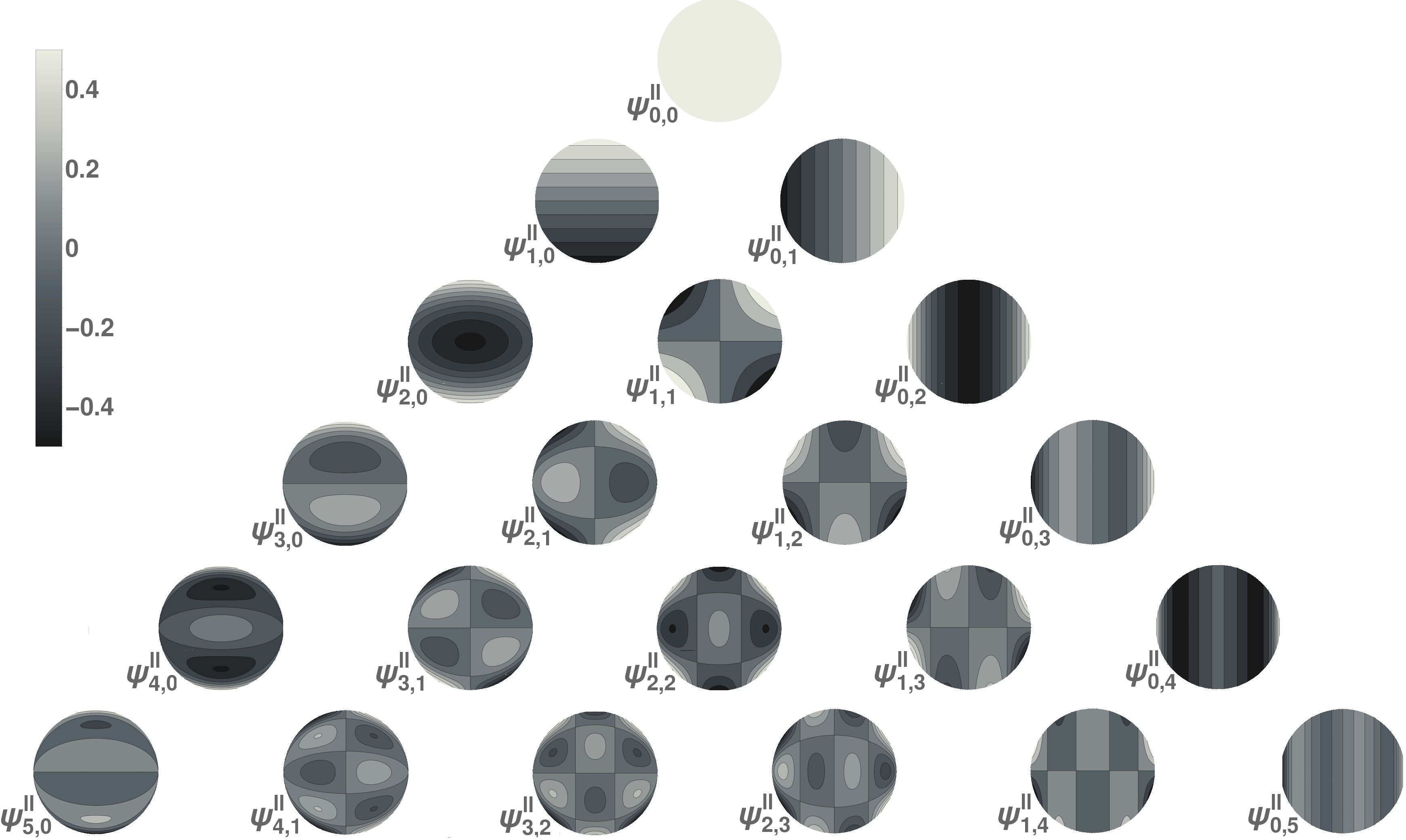
Figure 4: The new polynomial solutions to the Zernike quantum system on the disk $\cal D$, $\Psi^{\scriptscriptstyle\rm II}_{n_{1},n_{2}}(x,y)$ in (71), with rows of the same principal quantum number $n=n_{1}+n_{2}$. There are ten tones of gray between contours to emphasize the separating coordinates.

The Zernike differential equation (1) was found rather easily to separate in polar coordinates $(r,\phi)$, where for the Zernike values $(\alpha,\beta)=(-1,-2)$, the radial part was (12). Having here separated its solutions by coordinates $(u,v):=(x,\,y/\sqrt{1-x^{2}})$ that are shown in Fig. 2 (middle), we see that the solutions can be written as $\Psi_{n_{1},n_{2}}(x,y)=U_{n_{1},n_{2}}{{\scriptstyle(}u{\scriptstyle)}}V_{n_{1}}{{\scriptstyle(}v{\scriptstyle)}}$, and the equation written in separated form as follows,

$$\begin{array}[]{l}\displaystyle(u^{2}{-}1)^{2}\frac{\partial^{2}\Psi}{\partial u^{2}}+3u(u^{2}{-}1)\frac{\partial\Psi}{\partial u}\\ \displaystyle{}\quad{}+(1{-}v^{2})\frac{\partial^{2}\Psi}{\partial v^{2}}-2v\frac{\partial\Psi}{\partial v}=E(u^{2}-1)\Psi.\end{array}$$ (72)

The disk $\cal D$ in $(x,y)$ is thus mapped on the square ${{\scriptstyle|}u{\scriptstyle|}}\leq 1$, ${{\scriptstyle|}v{\scriptstyle|}}\leq 1$ where the coordinates $(u,v)$ are orthogonal.

5.3 The system III in (45)

The same line of reasoning we followed above for Systems I and II, apply to the coordinate system III in (45) for the coordinates $(\vartheta^{\prime\prime},\varphi^{\prime\prime})$. There, the potential (39) also takes the form of an effective potential also of Pöschl-Teller type,

$$V^{\scriptscriptstyle\rm III}_{\scriptscriptstyle\rm eff}=-\frac{1}{8}\bigg{(}\frac{1}{\sin^{2}\vartheta^{\prime\prime}\cos^{2}\varphi^{\prime\prime}}-1\bigg{)}.$$ (73)

This potential stems from (61) through the exchange $\vartheta^{\prime}\to\vartheta^{\prime\prime}$ and $\varphi^{\prime}\to\varphi^{\prime\prime}+{\textstyle\frac{1}{2}}\pi$. The solution of the Schrödinger equation (38) in the coordinate system III, now has the separated form,

$$\Upsilon^{\scriptscriptstyle\rm III}_{l_{1},l_{2}}(\vartheta^{\prime\prime},\varphi^{\prime\prime})=C_{l_{1},l_{2}}\,\sin^{l_{1}+\frac{1}{2}}\vartheta^{\prime\prime}\cos^{\frac{1}{2}}\varphi^{\prime\prime}\,C^{l_{1}+1}_{l_{2}}(\cos\vartheta^{\prime\prime})\,P_{l_{1}}(\sin\varphi^{\prime\prime}),$$ (74)

with $l_{1},l_{2}\in\{0,1,2,\ldots\}$, the same constant (69) and principal quantum number $n=l_{1}+l_{2}$. The energy spectrum is also given by $\cal E$ in (53).

The additional operator that describes the separation of solutions in the System III is

$$\begin{array}[]{rcl}\hat{J}_{2}\Upsilon^{\scriptscriptstyle\rm III}_{l_{1},l_{2}}(\vartheta^{\prime\prime},\varphi^{\prime\prime})&:=&\displaystyle\bigg{(}\frac{\partial^{2}}{\partial\varphi^{\prime\prime 2}}+\frac{1}{4\cos^{2}\varphi^{\prime\prime}}\bigg{)}\Upsilon^{\scriptscriptstyle\rm III}_{l_{1},l_{2}}(\vartheta^{\prime\prime},\varphi^{\prime\prime})\\[8.0pt] &=&\displaystyle\bigg{(}\hat{L}_{2}^{2}+\frac{\xi_{1}^{2}+\xi_{3}^{2}}{4\xi_{3}^{2}}\bigg{)}\Upsilon^{\scriptscriptstyle\rm III}_{l_{1},l_{2}}(\vartheta^{\prime\prime},\varphi^{\prime\prime})=-l^{2}\Upsilon^{\scriptscriptstyle\rm III}_{l_{1},l_{2}}(\vartheta^{\prime\prime},\varphi^{\prime\prime})\end{array}$$ (75)

where $l:=l_{1}+{\textstyle\frac{1}{2}}$. The expression of the wavefunctions (74) in the original coordinates $(x,y)$ on the disk, using $\cos\vartheta^{\prime\prime}=y$ and $\cos\varphi^{\prime\prime}=x/\sqrt{1-y^{2}}$, is

$$\Psi_{l_{1},l_{2}}(x,y)=C_{l_{1},l_{2}}(1-y^{2})^{l_{1}/2}\,P_{l_{1}}\Big{(}\frac{x}{\sqrt{1-y^{2}}}\Big{)}\,C^{l_{1}+1}_{l_{2}}(y).$$ (76)

This coincides with (71) under the rotation $x\to y$ and $y\to-x$ which connects systems II and III. The density plots of $\Psi_{l_{1},l_{2}}(x,y)$ are thus identical to those in Fig. 4, except for a ${\textstyle\frac{1}{2}}\pi$ rotation of the disks.

6 The superintegrable algebra of Zernike

The two operators that determined the constans of motion, $\hat{J}_{1}$ in (70) and $\hat{J}_{2}$ in (75), were written in terms of the angular momentum operators $\hat{L}_{i}$ in (35). We can add the angular momentum $\hat{L}_{3}$ in (25) and (35) as a third one, and thus have

$${\hat{J}_{1}}=\hat{L}_{1}^{2}+\frac{\xi_{2}^{2}+\xi_{3}^{2}}{4\xi_{3}^{2}},\quad{\hat{J}_{2}}=\hat{L}_{2}^{2}+\frac{\xi_{1}^{2}+\xi_{3}^{2}}{4\xi_{3}^{2}},\quad{\hat{J}_{3}}=\hat{L}_{3},$$ (77)

and thereby write the operator $\widehat{W}$ in (33) as

$$\widehat{W}={\hat{J}_{1}}+{\hat{J}_{2}}+{\hat{J}_{3}^{2}}+{\textstyle\frac{1}{2}}.$$ (78)

To complete this algebra, we construct a third linearly independent operator out of the commutator of the previous two,

$$\hat{S}_{1}={\hat{J}_{3}},\qquad\hat{S}_{2}=\hat{J}_{1}-\hat{J}_{2},\qquad\hat{S}_{3}=[\hat{S}_{1},\hat{S}_{2}]$$ (79)

which now satisfy the the following relations:

$$\hat{S}_{3}=2\{\hat{L}_{1},\hat{L}_{2}\}_{\scriptscriptstyle\rm\!+}-\frac{\xi_{1}\xi_{2}}{\xi_{3}^{2}},\quad[\hat{S}_{3},\hat{S}_{1}]=4\hat{S}_{2},\quad[\hat{S}_{3},\hat{S}_{2}]=8\hat{S}_{1}^{3}-8\widehat{W}\hat{S}_{1},$$ (80)

where $\{\,,\,\}_{\scriptscriptstyle\rm\!+}$ is the anticommutator. Thus, the operators $\hat{S}_{1},\hat{S}_{2},\hat{S}_{3}$ a generate nonlinear algebra, called the cubic or Higgs algebra [7].

To write the three operators that commute with Zernike operator $\hat{Z}$ in the original configuration space $(x,y)$, we must undo the similarity transformation in (29) for the symmetry operators $\hat{K}_{i}=A^{-1}\hat{S}_{i}A$, thus obtaining three constants of the motion,

$$\hat{K}_{1} = y\partial_{x}-x\partial_{y},$$ (81)

$$\hat{K}_{2} = -(1-x^{2}-y^{2})(\partial_{xx}-\partial_{yy})+2x\partial_{x}-2y\partial_{y},$$ (82)

$$\hat{K}_{3} = -4(1-x^{2}-y^{2})\partial_{xy}+4y\partial_{x}+4x\partial_{y},$$ (83)

which close into the algebra

$$[\hat{K}_{1},\hat{K}_{2}]=\hat{K}_{3},\quad[\hat{K}_{3},\hat{K}_{1}]=4\hat{K}_{2},\quad[\hat{K}_{3},\hat{K}_{2}]=8(\hat{K}_{1}^{3}-\hat{Z}\hat{K}_{1}).$$ (84)

The three operators (81)–(83) separate in the coordinate systems introduced in (43)–(45).

7 Concluding remarks

We have introduced the quantum Zernike system defined by the Hamiltonian (1) that naturally separates in polar coordinates. This Hamiltonian is nonstandard because it involves a quadratic re-scaling potential term, and its wavefunctions have nonzero values at its finite circular boundary.

We have shown that this two-dimensional system can also be separated in two additional coordinate systems, where the Zernike Hamiltonian takes the form of quantum mechanical Schrödinger Hamiltonians with Pöschl-Teller potentials, whose solutions involve separated Legendre and Gegenbauer polynomials. These coordinate systems become evident when orthogonal coordinates on a half-sphere are mapped as non-orthogonal coordinates on the disk. The boundary condition on the disk requires one additional limit that the solutions on the half-sphere must satisfy. Associated to the separable coordinate systems, there are operators whose eigenvalues are constants of the motion. Previously only the angular momentum of circular harmonics was known; this, plus the two new operators stemming from separability, yielded three operators that commute with the Zernike Hamiltonian, and close into a cubic Higgs superalgebra.

We realize that the analysis performed here on the sphere can be generalized. First, also the elliptical system of coordinates on the sphere and its projections [16, 12, 13] can be used to separate the Zernike equation and provide solutions on one more system of coordinates. Interbasis expansions will then relate the Zernike functions on the disk with Legendre and Gegenbauer polynomials as well as Lamé functions. We leave this as a separate analysis to be studied elsewhere. We also note that instead of unit radius and $\alpha_{\scriptscriptstyle\rm Z}=-1$, we may have a self-adjoint Hamiltonian when the circular boundary is at $r=1/\sqrt{{{\scriptstyle|}\alpha{\scriptstyle|}}}$, provided that $\beta=-2{{\scriptstyle|}\alpha{\scriptstyle|}}$. Finally, one can disregard the boundary problem and revert to the full parameter ranges of $\alpha$ and $\beta$, such as was done in Ref. [17] and obtain solutions that correspond to open hyperbolic trajectories and, more generally, study Schrödinger equations that stem from quadratic extensions of the oscillator algebra. The methods of solution and mathematical structure can be along the lines of this research.

References

- [1] D. Basu and K. B. Wolf, The Clebsch-Gordan coefficients of the three-dimensional Lorentz algebra in the parabolic basis, J. Math. Phys. 24, 478–500 (1983).
- [2] A. B. Bhatia and E. Wolf, On the circle polynomials of Zernike and related orthogonal sets, Math. Proc. Cambridge Phil. Soc. 50, 40–48 (1954).
- [3] M. Born and E. Wolf, Principles of Optics: Electromagnetic Theory of Propagation, Interference and Diffraction of Light 7th ed. (Cambridge University Press, 1999). p. 986.
- [4] W. M. Frank and D. J. Land, Singular potentials, Rev. Mod. Phys. 43, 36–98 (1971).
- [5] I. S. Gradshteyn and I. M. Ryzhik, Table of Integrals, Series and Products, 7th Ed. (Elsevier, 2007), ISBN-13: 978-0-12-373637-6.
- [6] C. Grosche, G. S. Pogosyan, and A. N. Sissakian, Path integral discussion for Smorodinsky-Winternitz potentials II. Two- and three-dimensional sphere, Fortschr. Phys. 43, 453–521 (1995).
- [7] P. W. Higgs, Dynamical symmetries in a spherical geometry, J. Phys. A 12, 309–323 (1979).
- [8] M. E. H. Ismail and R. Zhang, Classes of bivariate orthogonal polynomials, arXiv:1502.07256v3 [math.CA].
- [9] E. G. Kalnins, W. Miller Jr., and G. S. Pogosyan, Superintegrability and associated polynomial solutions. Euclidean space and sphere in two-dimensions space and sphere, J. Math. Phys. 37, 6439–6467 (1996).
- [10] E. G. Kalnins, J. M. Kress, W. Miller Jr., and G. S. Pogosyan, Completeness of superintegrability in two-dimensional constant curvature spaces, J. Phys. A 34, 4705–4720 (2001).
- [11] E. C. Kintner, On the mathematical properties of the Zernike Polynomials, Opt. Acta 23, 679–680 (1976).
- [12] I. Lukač and Ya. A. Smorodinskiĭ, Wave functions for the asymmetric top, Sov. Phys. JETP 30, 728–730 (1970).
- [13] I. Lukach, A complete set of the quantum-mechanical observables on a two-dimensional sphere, Theor. Math. Phys. 14, 271–281 (1973).
- [14] W. Miller Jr., Symmetry and Separation of Variables, Encyclopedia of Mathematics and its Applications, Vol. 4, Ed. by G.-C. Rota (Cambridge University Press, 1977).
- [15] D. R. Myrick, A Generalization of the radial polynomials of F. Zernike, SIAM J. Appl. Math. 14, 476–489 (1966).
- [16] G. S. Pogosyan, A. N. Sissakian and P. Winternitz, Separation of variables and Lie algebra contractions. Applications to special functions, Phys. Part. Nuclei 33, Suppl. 1, S123–S144 (2002).
- [17] G. S. Pogosyan, K. B. Wolf, and A. Yakhno, Superintegrable classical Zernike system, J. Math. Phys. , submitted (2017).
- [18] B. H. Shakibaei and R. Paramesran, Recursive formula to compute Zernike radial polynomials, Opt. Lett. 38, 2487–2489 (2013).
- [19] A. Wünsche, Generalized Zernike or disc polynomials, J. Comp. App. Math. 174, 135–163 (2005).
- [20] F. Zernike, Beugungstheorie des Schneidenverfahrens und Seiner Verbesserten Form der Phasenkontrastmethode, Physica 1, 689–704 (1934).