Abstract

We consider the differential equation that Zernike proposed to classify aberrations of wavefronts in a circular pupil, as if it were a classical Hamiltonian with a non-standard potential. The trajectories turn out to be closed ellipses. We show that this is due to the existence of higher-order invariants that close into a cubic Higgs algebra. The Zernike classical system thus belongs to the class of superintegrable systems. Its Hamilton-Jacobi action separates in three vertical projections of polar coordinates of a sphere, polar and equidistant coordinates on half-hyperboloids, and also in elliptic coordinates on the sphere.

1 Introduction: the Zernike operator

In Reference [23, p. 700], Frits Zernike proposed a two-dimensional differential equation whose polynomial solutions provide an orthogonal basis for functions $f{{\scriptstyle(}{\bf r}{\scriptstyle)}}$ in a Hilbert space ${\cal L}^{2}_{\scriptscriptstyle\rm Z}({\cal D}_{1})$ over the unit disk ${\bf r}\in{\cal D}_{1}$, ${{\scriptstyle|}{\bf r}{\scriptstyle|}}\leq 1$ which —importantly— have a constant absolute value on the boundary circle: $|f({\bf r})|_{{{\scriptstyle|}{\bf r}{\scriptstyle|}}{=}1}=1$. This Zernike basis is thus distinct from the well-known bases of Bessel functions over the disk whose values (or logarithmic derivatives) vanish on a boundary circle. The differential operator and eigenvalue equation of Zernike are

$$\hat{Z}^{(\alpha,\beta)}f{{\scriptstyle(}{\bf r}{\scriptstyle)}}:=\Big{(}\nabla^{2}+\alpha({\bf r}\cdot\nabla)^{2}+\beta\,{\bf r}\cdot\nabla\Big{)}f{{\scriptstyle(}{\bf r}{\scriptstyle)}}=-E\,f{{\scriptstyle(}{\bf r}{\scriptstyle)}}.$$ (1)

The requirement that this operator be self-adjoint under the inner product $(f_{1},f_{2})_{{\cal D}_{1}}:=\int_{{\cal D}_{1}}{\rm d}^{2}{\bf r}\,f_{1}{{\scriptstyle(}{\bf r}{\scriptstyle)}}^{*}\,f_{2}{{\scriptstyle(}{\bf r}{\scriptstyle)}}$, i.e., $(\hat{Z}f_{1},f_{2})_{{\cal D}_{1}}=(f_{1},\,\hat{Z}\,f_{2})_{{\cal D}_{1}}$, constrains the coefficients to have the values $(\alpha_{\scriptscriptstyle\rm Z},\beta_{\scriptscriptstyle\rm Z}):=(-1,-2)$ [23]. In this paper however, we let $\alpha$ and $\beta$ take arbitrary real values, to be later constrained to those regions that lead to the closed orbits that we consider to be the main feature of interest of the Zernike system.

For $\hat{Z}^{(\alpha_{\scriptscriptstyle\rm Z},\beta_{\scriptscriptstyle\rm Z})}$ in (1), the polar factored solutions $Z_{n,m}(r)\exp({\rm i}m\phi)$, $|m|\leq n$, correspond to the eigenvalues $E=n(n+2)$; when normalized to $Z_{n,m}(1)=1$, the radial functions are the Zernike polynomials [23]. These can be related to the Jacobi polynomials $\sim P_{n}^{(m-n,0)}(2r^{2}-1)$ whose interval of orthogonality is $|_{-1}^{1}\leftrightarrow r|_{0}^{1}$. It was remarked in Ref. [2] that the reasons for postulating Eq. (1) were rather arbitrary, so its authors used the Gram-Schmidt method to find the same polynomial solutions from first principles. Zernike polynomials have wide applications in the correction of optical aberrations by describing wavefronts at circular pupils (see for example Ref. [3]); they also display a host of enticing mathematical properties [13, 9, 18, 20, 22, 8] that are characteristic of algebraic structures.

When $\alpha=0$, $\hat{Z}^{(0,\beta)}$ reduces to a linear combination of generators of the real symplectic algebra ${\sf sp(}$4${\sf,R)}$ under Poisson brackets or commutators [21, Sect. 11.4]; when also $\beta=0$, then (1) becomes simply the Laplace equation with plane wave solutions $\sim\exp({\rm i}{\bf k}\cdot{{\bf r}})$, $|{\bf k}|^{2}=E$ or, adapted to polar coordinates $(r,\phi)$, multipole solutions $\sim J_{m}(kr)e^{{\rm i}m\phi}$ with Bessel functions, where the radial wavenumber $k$ may or may not be quantized according to whether the boundary conditions are set at a finite or infinite radius. On the other hand, when $\alpha\neq 0$ but $\beta=0$, the Zernike equation (1) reduces to the kinetic part of a nonlinear oscillator Hamiltonian [4]. We shall keep their generic values $(\alpha,\beta)\in{\cal R}^{2}$ and particularize when convenient.

We found that it is of interest to examine the classical counterpart of the Zernike system, which in ‘wave’ (or quantum mechanical) form is (1). The process of de-quantization of this equation consists in replacing

$$\nabla\mapsto{\rm i}{\bf p}={\rm i}\left(\matrix{\displaystyle{p_{x}}{}_{\mathstrut}\cr\displaystyle{p_{y}}\cr}\right), {\bf r}=\left(\matrix{\displaystyle{x}{}_{\mathstrut}\cr\displaystyle{y}\cr}\right),\quad r:={{\scriptstyle|}{\bf r}{\scriptstyle|}},$$ (2)

$$\nabla^{2}\mapsto-(p_{x}^{2}+p_{y}^{2})=-\bigg{(}p_{r}^{2}+\frac{p_{\phi}^{2}}{r^{2}}\bigg{)}, {\bf r}\cdot\nabla\mapsto{\rm i}(xp_{x}+yp_{y})={\rm i}\,rp_{r}.$$ (3)

The operator (1) thus yields a classical Hamiltonian function $H^{(\alpha,\beta)}=-\hat{Z}^{(\alpha,\beta)}$ which depends on two coordinates and two momenta. In Cartesian and polar coordinates, it is

$$H^{(\alpha,\beta)} := (p_{x}^{2}+p_{y}^{2})+\alpha(xp_{x}+yp_{y})^{2}-{\rm i}\beta(xp_{x}+yp_{y})$$ (4)

$$= (1+\alpha r^{2})p_{r}^{2}+p_{\phi}^{2}/r^{2}-{\rm i}\beta rp_{r},$$ (5)

and its value is the energy $E$. The appearance of ${\rm i}=\sqrt{-1}$ in this Hamiltonian seems indeed anomalous, yet our calculations will show that at the end we have a purely real classical system whose trajectories can be found explicitly.

The Hamilton-Jacobi method is particularly apt to solve this system, where we shall preferentially use the polar coordinates $(r,\phi)$ and their momenta $(p_{r},p_{\phi})$ in (5). Since $H^{(\alpha,\beta)}=E$ is independent of time and the angular coordinate $\phi$ is cyclic, the action function $S(r,\phi)$ (also called Hamilton’s principal function) that satisfies the Hamilton-Jacobi equation $H+\partial S/\partial t=0$ can be separated in the form

$$S(r,\phi)=R{{\scriptstyle(}r{\scriptstyle)}}+p_{\phi}\phi-Et.$$ (6)

The space derivatives of this function yield the polar momenta $p_{r}$ and $p_{\phi}$ as

$$p_{r}=\frac{\partial S(r,\phi)}{\partial r},\quad r=-\frac{\partial S(r,\phi)}{\partial p_{r}},\qquad p_{\phi}=\frac{\partial S(r,\phi)}{\partial\phi},\quad\phi=-\frac{\partial S(r,\phi)}{\partial p_{\phi}}.$$ (7)

In Sect. 2 we shall use the derivatives of (6) with respect to the radius $r$ and the angle $\phi$, to find the geometric trajectories $r(\phi)$, which are closed ellipses. Then in Sect. 3 the dynamical trajectories ${\bf r}(t)$ will be found differentiating the action $S(r,\phi)$ with respect to the energy. The symmetries behind the closure of the orbits will be elucidated in Sect. 4, where Eq. (1) is separated in three spherical, six hyperbolic, and elliptic coordinates, and shown to lead to constants of motion. In Sect. 5 we show that the operators which characterize these constants close into a cubic superintegrable algebra, and offer some additional comments.

2 Geometric trajectories $r(\phi)$

The derivative of the action function (6) with respect to the radius $r$ is the radial momentum,

$$p_{r}=\frac{\partial S(r,\phi)}{\partial r}=\frac{\partial R{{\scriptstyle(}r{\scriptstyle)}}}{\partial r}.$$ (8)

Replacing $p_{r}$ in (5) yields a quadratic algebraic equation for the derivative of $R{{\scriptstyle(}r{\scriptstyle)}}$, namely

$$(1+\alpha r^{2})\bigg{(}\frac{\partial R{{\scriptstyle(}r{\scriptstyle)}}}{\partial r}\bigg{)}^{2}-{\rm i}\beta r\bigg{(}\frac{\partial R{{\scriptstyle(}r{\scriptstyle)}}}{\partial r}\bigg{)}+\frac{p_{\phi}^{2}}{r^{2}}=E,$$ (9)

whose two solutions are

$$\frac{\partial R{{\scriptstyle(}r{\scriptstyle)}}}{\partial r}=\frac{{\rm i}\beta\,r\pm\sqrt{-\beta^{2}r^{2}-4(1+\alpha r^{2})(p_{\phi}^{2}/r^{2}-E)}}{2(1+\alpha r^{2})}.$$ (10)

From here we find $R{{\scriptstyle(}r{\scriptstyle)}}$ through the indefinite integral

$$R{{\scriptstyle(}r{\scriptstyle)}}=\int{\rm d}r\left(\frac{{\rm i}\beta\,r}{2(1+\alpha r^{2})}\pm\frac{\sqrt{(\alpha E{-}{\textstyle\frac{1}{4}}\beta^{2})r^{2}+(E{-}\alpha p_{\phi}^{2})-p_{\phi}^{2}/r^{2}}}{1+\alpha r^{2}}\right).$$ (11)

We can now find the trajectories that relate $r$ and $\phi$ by differentiating (6) with respect to $p_{\phi}$,

$$\frac{\partial S(r,\phi)}{\partial p_{\phi}}=\frac{\partial R{{\scriptstyle(}r{\scriptstyle)}}}{\partial p_{\phi}}+\phi=\phi_{o},$$ (12)

where $\phi_{o}$ is a constant of the motion given by the initial conditions. The derivative of $R{{\scriptstyle(}r{\scriptstyle)}}$ in (11) with respect to $p_{\phi}$, is then

$$\frac{\partial R{{\scriptstyle(}r{\scriptstyle)}}}{\partial p_{\phi}} = \pm\int{\rm d}r\,\frac{\partial}{\partial p_{\phi}}\frac{\sqrt{(\alpha E{-}{\textstyle\frac{1}{4}}\beta^{2})r^{2}-(\alpha+1/r^{2})p_{\phi}^{2}+E}}{1+\alpha r^{2}}$$ (13)

$$= \mp p_{\phi}\int\frac{{\rm d}r}{r}\,\frac{1}{\sqrt{(\alpha E{-}{\textstyle\frac{1}{4}}\beta^{2})r^{4}+(E-\alpha p_{\phi}^{2})r^{2}-p_{\phi}^{2}}}$$ (14)

$$= \mp\frac{p_{\phi}}{2}\int{\rm d}z\,\frac{1}{z\sqrt{a+b\,z+c\,z^{2}}}$$ (15)

where in the last equality we have substituted $z=r^{2}$ with ${\rm d}r/r={\textstyle\frac{1}{2}}{\rm d}z/z$, and we define

$$a:=-p_{\phi}^{2},\quad b:=E-\alpha p_{\phi}^{2},\quad c:=\alpha E-{\textstyle\frac{1}{4}}\beta^{2}.$$ (16)

We note that the imaginary summand in (11) is absent from this equation and thus from the system. The double sign in (13) corresponds to the $\pm p_{\phi}$ angular momentum of a trajectory traversed in opposite directions.

One finds the indefinite integral solved in [6, Eqs. 2.266], with various expressions involving inverse trigonometric and hyperbolic functions, or logarithms, depending on the signs of the constants; in our case (16) $a<0$ and for $b^{2}-4ac=(E+\alpha p_{\phi}^{2})^{2}-\beta^{2}p_{\phi}^{2}>0$, the integral is

$$\int{\rm d}z\,\frac{1}{z\sqrt{a+b\,z+c\,z^{2}}}=\frac{1}{\sqrt{-a}}\arcsin\frac{2a+bz}{z\sqrt{b^{2}-4ac}}.$$ (17)

Thus, joining Eqs. (12), (16), and (17), we obtain

$$\phi-\phi_{o}=-\frac{\partial R{{\scriptstyle(}r{\scriptstyle)}}}{\partial p_{\phi}}=\frac{1}{2}\arcsin\frac{(E-\alpha p_{\phi}^{2})r^{2}-2p_{\phi}^{2}}{r^{2}\sqrt{(E+\alpha p_{\phi}^{2})^{2}-\beta^{2}p_{\phi}^{2}}},$$ (18)

and this leads to $\phi(r^{2})$ in the form

$$\sin 2(\phi{-}\phi_{o})=\frac{Ar^{2}-B}{Cr^{2}},\quad\left\{\begin{array}[]{l}A:=E-\alpha p_{\phi}^{2},\\ B:=2p_{\phi}^{2},\\ C:=\sqrt{(E+\alpha p_{\phi}^{2})^{2}-\beta^{2}p_{\phi}^{2}}.\end{array}\right.$$ (19)

We can invert the dependence to $r(\phi)$ by solving for the square radius and setting for convenience $\phi_{o}=-\frac{1}{4}\pi$,

$$r^{2}(\phi) = \frac{B}{A-C\cos 2\phi}=\frac{2p_{\phi}^{2}}{\displaystyle(E{-}\alpha p_{\phi}^{2})-\sqrt{(E{+}\alpha p_{\phi}^{2})^{2}-\beta^{2}p_{\phi}^{2}}\,\cos 2\phi}$$ (20)

$$= \frac{D}{1-\varepsilon\cos 2\phi},\quad\left\{\begin{array}[]{l}D:=B/A=2p_{\phi}^{2}/(E{-}\alpha p_{\phi}^{2}),\quad E\neq\alpha p_{\phi}^{2},\\[3.0pt] \displaystyle\,\varepsilon\,:=\frac{C}{A}=\frac{\sqrt{(E+\alpha p_{\phi}^{2})^{2}-\beta^{2}p_{\phi}^{2}}}{E-\alpha p_{\phi}^{2}}.\end{array}\right.$$ (23)

This is the parametric equation for ellipses, provided that

$$\begin{array}[]{lclcl}\varepsilon\hbox{ real}&\Rightarrow&C^{2}\geq 0&\Rightarrow&\displaystyle\left\{\begin{array}[]{l}E\leq-\alpha p_{\phi}^{2}-|\beta p_{\phi}|,\\ E\geq-\alpha p_{\phi}^{2}+|\beta p_{\phi}|,\end{array}\right.\\ {{\scriptstyle|}\varepsilon{\scriptstyle|}}<1&\Rightarrow&A^{2}>C^{2}&\Rightarrow&\quad\,4\alpha E<\beta^{2},\\ r^{2}(\phi)>0&\Rightarrow&D>0&\Rightarrow&\quad\,E>\alpha p_{\phi}^{2}.\end{array}$$ (24)

These conditions restrict the range of energies $E$ and angular momenta $p_{\phi}$ where the trajectories are real and closed. As shown in Fig. 1 (left) for the generic Zernike range $\alpha<0$, $\beta\neq 0$, the first condition excludes the energy interval between the two parabolas, $-\alpha\,p_{\phi}^{2}-|\beta\,p_{\phi}|\leq E\leq-\alpha\,p_{\phi}^{2}+|\beta\,p_{\phi}|$; the second inequality is (for $\alpha<0$) a lower bound $E>-\beta^{2}/4|\alpha|$ (equal to $-1$ for the Zernike case); lastly, the third condition excludes the interior of the parabola $E=\alpha p_{\phi}^{2}$ that has its apex at the origin, and which eliminates the region $|p_{\phi}|<-{\textstyle\frac{1}{2}}|\beta|/\alpha$ that was left allowed by the previous two conditions.

In Fig. 1 (right) we show the allowed regions for the generic Zernike range $\alpha>0$, $\beta\neq 0$. The two parabolas stemming from the first inequality in (24), under $\alpha\leftrightarrow-\alpha$ reflect the $E$-axis; the second inequality in (24) is now the upper bound $E<\beta^{2}/4\alpha$; and the third inequality allows elliptic orbits in the remaining interior of the parabola, namely $-\alpha p_{\phi}^{2}+|\beta p_{\phi}|<E<\beta^{2}/4\alpha$ for $0\leq|p_{\phi}|<|\beta|/2\alpha$. Finally, when $\alpha=0$, the ‘forbidden’ region between the two parabolas due to the first condition in (24) becomes $-|\beta p_{\phi}|\leq E\leq|\beta p_{\phi}|$, while the second two conditions are satisfied by $E>0$, so that closed elliptical trajectories occur for all $E\geq|\beta p_{\phi}|$ .

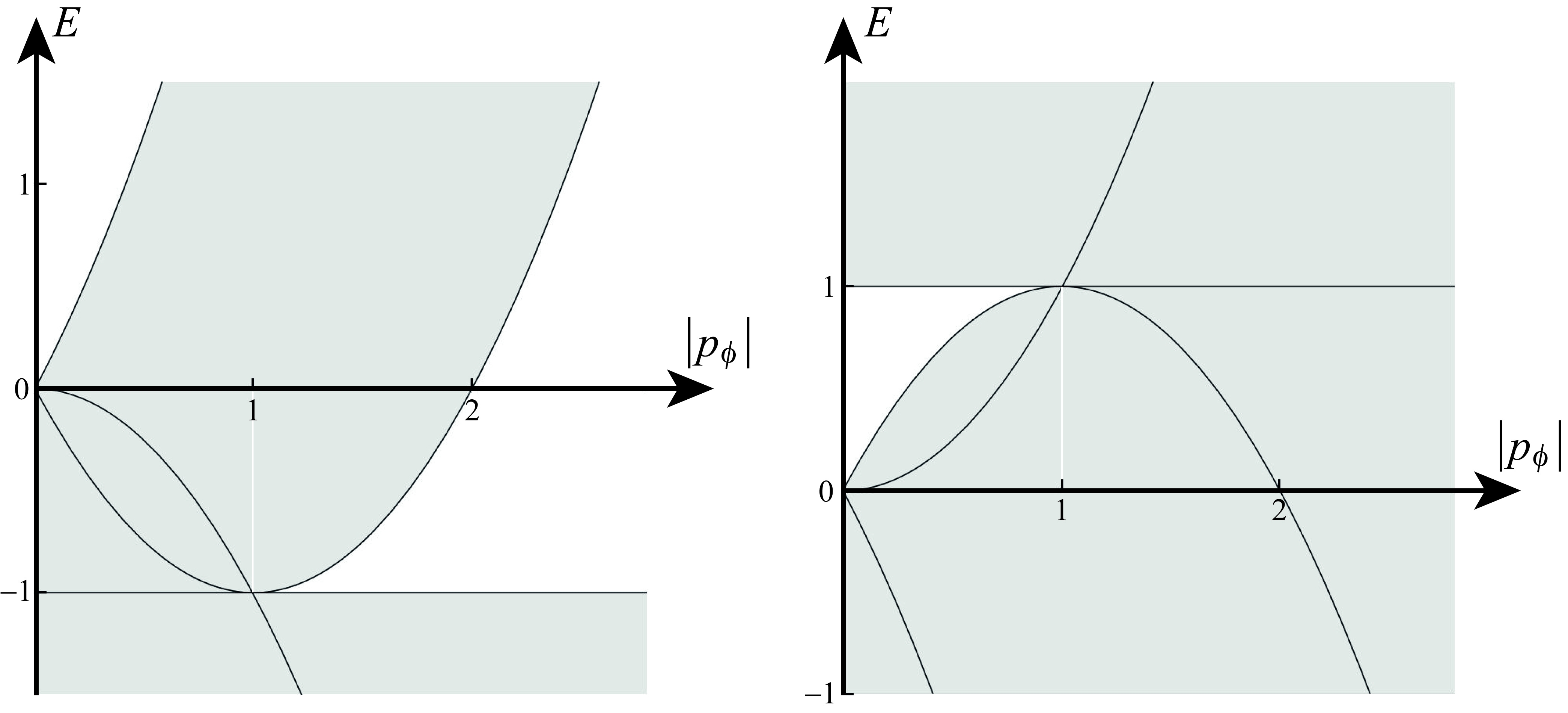
Figure 1: Regions of the plane of angular momentum $p_{\phi}$ and energy $E$, where closed trajectories are allowed by the inequalities (24) (in white) for $(\alpha,\beta)$-Zernike systems. Left: Allowed regions for the original Zernike system $(\alpha_{\scriptscriptstyle\rm Z},\beta_{\scriptscriptstyle\rm Z})=(-1,-2)$. Right: Allowed regions for $(\alpha,\beta)=(1,2)$. Closed elliptical trajectories do not occur in the gray regions. The structure of these regions is generic for all $\alpha$ and $\beta\neq 0$. The units of $E$ in these graphs are $\beta^{2}/4|\alpha|$ and the units of $|p_{\phi}|$ are $\frac{1}{2}|\beta/\alpha|$.

Since we took $\phi_{o}=-\frac{1}{4}\pi$, the $y$-axis is at $\phi=0$ and the $x$-axis at $\phi=\frac{1}{2}\pi$. The semi-major and semi-minor axes of the ellipse are, respectively,

$$\mu_{y}:=\sqrt{\frac{D}{1-\varepsilon}}=\sqrt{\frac{B}{A-C}},\quad\mu_{x}:=\sqrt{\frac{D}{1+\varepsilon}}=\sqrt{\frac{B}{A+C}}.$$ (25)

The area of this ellipse is given by $\pi$ times the product of the two semi-axes,

$$\hbox{area}=\pi\mu_{x}\mu_{y}=\frac{\pi D}{\sqrt{1{-}\varepsilon^{2}}}=\frac{\pi B}{\sqrt{A^{2}{-}C^{2}}}=\frac{2\pi\,|p_{\phi}|}{\sqrt{\beta^{2}-4\alpha E}}.$$ (26)

3 Dynamical trajectories $r(t)$ and orbits

We return now to the integral expression for $R{{\scriptstyle(}r{\scriptstyle)}}$ in (11), differentiating the action $S(r,\phi)$ in (6) now with respect to the energy $E$,

$$\frac{\partial S(r,\phi)}{\partial E}=\frac{\partial R{{\scriptstyle(}r{\scriptstyle)}}}{\partial E}-t=-t_{o},$$ (27)

where $t_{o}$ is the initial time constant. Instead of (13)–(15), we now have

$$\frac{\partial R{{\scriptstyle(}r{\scriptstyle)}}}{\partial E} = \pm\int{\rm d}r\,\frac{\partial}{\partial E}\frac{\sqrt{(\alpha E{-}{\textstyle\frac{1}{4}}\beta^{2})r^{2}-(\alpha+1/r^{2})p_{\phi}^{2}+E}}{1+\alpha r^{2}}$$ (28)

$$= \pm\frac{1}{2}\int{\rm d}r\,\frac{1}{\sqrt{(\alpha E{-}{\textstyle\frac{1}{4}}\beta^{2})r^{2}-(\alpha+1/r^{2})p_{\phi}^{2}+E}}$$ (29)

$$= \pm\frac{1}{4}\int{\rm d}z\,\frac{1}{\sqrt{a+b\,z+c\,z^{2}}}$$ (30)

where as before we have set $z=r^{2}$, and $a,\,b,\,c$ are again given by (16). The indefinite integral can be found in [6, Eqs. 2.261]; it is

$$\int{\rm d}z\,\frac{1}{\sqrt{a+b\,z+c\,z^{2}}}=\frac{-1}{\sqrt{-c}}\arcsin\frac{2cz+b}{\sqrt{b^{2}-4ac}},$$ (31)

The conditions for this integral to be proper, $c<0$ and $b^{2}-4ac>0$ also lead to (24), while the solutions corresponding to (19) are now

$$\sin\Big{(}4(t{-}t_{o})\sqrt{U}\Big{)}=\frac{A-2U\,r(t)^{2}}{C},\quad U:={\textstyle\frac{1}{4}}\beta^{2}-\alpha E=\frac{A^{2}-C^{2}}{2B}>0,$$ (32)

with $A$ and $C$ given by (19).

From here we can extract the dependence of the square radius of the trajectory on time as (23) did for the angle. We choose $t_{o}$ such that $r(t)|_{t=0}=\mu_{y}$ is the semi-major axis in (25), i.e., $4t_{o}\surd U={\textstyle\frac{1}{2}}\pi$, so $t_{o}=\frac{1}{8}\pi/\surd U$, and write

$$\begin{array}[]{rcl}r^{2}(t)&=&\displaystyle\frac{A+C\cos(4t\sqrt{U})}{2U}\\ &=&\displaystyle\frac{E+\displaystyle\sqrt{(E{+}\alpha p_{\phi}^{2})^{2}{-}\beta^{2}p_{\phi}^{2}}\,\cos(2t\sqrt{\beta^{2}{-}4\alpha E})-\alpha p_{\phi}^{2}}{{\textstyle\frac{1}{2}}\beta^{2}-2\alpha E}.\end{array}$$ (33)

This is a periodic function of time, with period $4T\surd U=2\pi$, or

$$T=\pi\Big{/}\sqrt{\beta^{2}-4\alpha\,E}.$$ (34)

In the generalized Zernike range $\alpha<0$, the radicand is positive; when $\alpha>0$, the second inequality in (24) prevents the orbits from being closed for $\alpha E>\frac{1}{4}\beta^{2}$. Although orbits in the Zernike range are ellipses, they differ from the isochronous orbits of the classical harmonic oscillator, whose period does not depend on their energy [5].

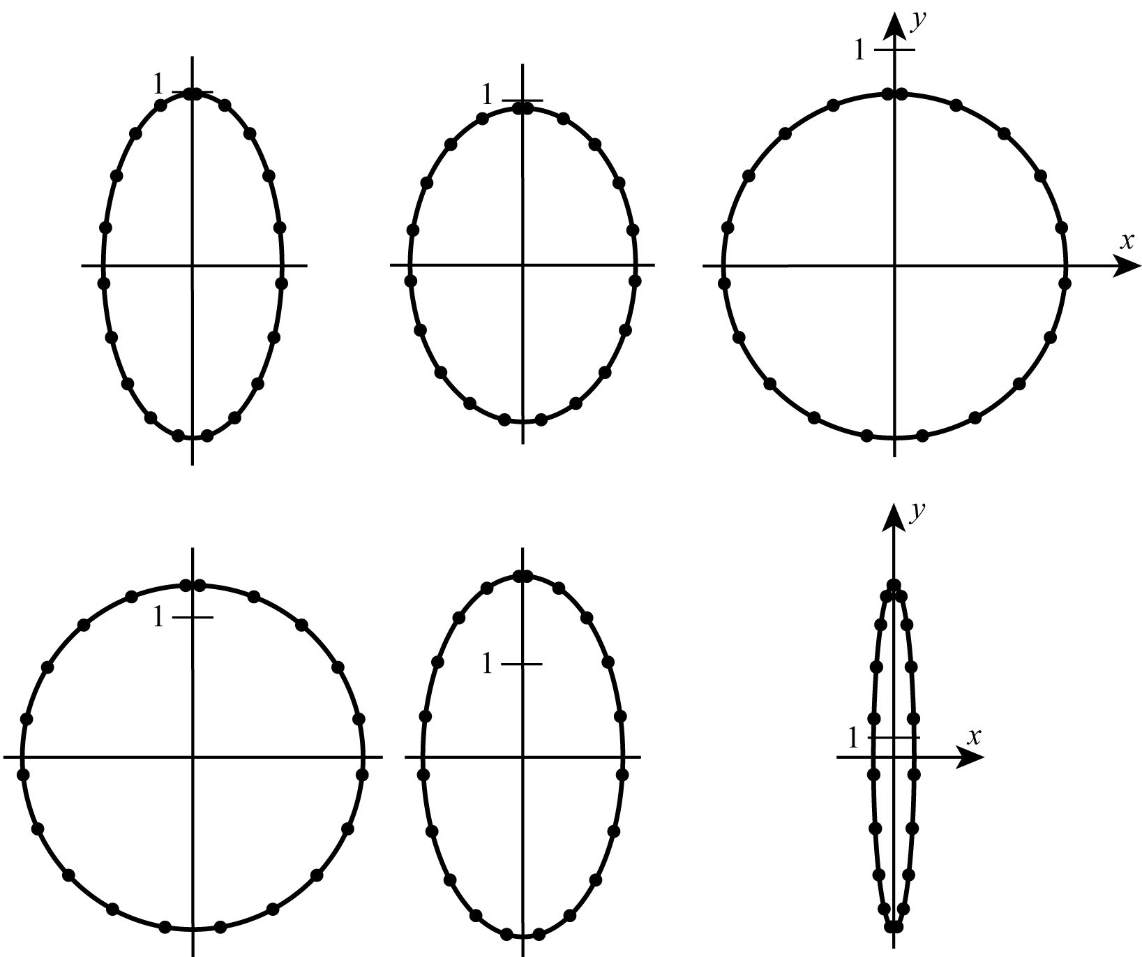
Figure 2: Trajectories $\Big{(}x(t),y(t)\Big{)}$ in the classical Zernike system $(\alpha_{\scriptscriptstyle\rm Z},\beta_{\scriptscriptstyle\rm Z})=(-1,-2)$ and angular momentum $p_{\phi}=3$, for equidistant times $t\in[0,T]$. Upper row: trajectories inside the disk ${\cal D}_{1}$ for energies $E=35$, 20, and 15 (at the lower boundary of the upper allowed region of Fig. 1). Lower row: trajectories outside the unit disk ${\cal D}_{1}$, for energies $E=3$ (at the upper boundary of the lower allowed region), 1, and $-0.9$ (near to the lower forbidden region), which fall completely outside the disk and correspond to the hyperbolic case to be seen in Sect. 4. We mark the scale 1 on the $y$-axis, understood to be in units of $1/\surd|\alpha|$.

As a function of time, the trajectories $\Big{(}x(t),\,y(t)\Big{)}$ can be found from the previous expressions, (23) and (33), as

$$x(t) = r\sin\phi=r\sqrt{{\textstyle\frac{1}{2}}(1{-}\cos 2\phi)}=\frac{1}{\sqrt{2\varepsilon}}\sqrt{(\varepsilon{-}1)\,r^{2}(t)+D}$$ (35)

$$= \frac{1}{\sqrt{2\varepsilon}}\sqrt{(\varepsilon{-}1)\frac{A+C\cos(4t\sqrt{U})}{2U}+D},$$

$$y(t) = r\cos\phi=r\sqrt{{\textstyle\frac{1}{2}}(1{+}\cos 2\phi)}=\frac{1}{\sqrt{2\varepsilon}}\sqrt{(\varepsilon{+}1)\,r^{2}(t)-D}$$ (36)

$$= \frac{1}{\sqrt{2\varepsilon}}\sqrt{(\varepsilon{+}1)\frac{A+C\cos(4t\sqrt{U})}{2U}-D},$$

and are shown in Fig. 2 for the Zernike case $(\alpha_{\scriptscriptstyle\rm Z},\beta_{\scriptscriptstyle\rm Z})=(-1,-2)$, but are valid for the range $\alpha<0$.

The trajectories are circular when $\varepsilon=0$, i.e., $C=0$ or $E+\alpha p_{\phi}^{2}=\pm|\beta\,p_{\phi}|$. This is the case of the upper right and lower left trajectories in Fig. 2. For $\alpha<0$ it occurs on the two parabolas that bound the region excluded by the first condition in (24) and respect the other two inequalities. The radius of those circles can be found from (23), as $r^{2}(\phi)=D$. At the upper boundary one has $E=-\alpha p_{\phi}^{2}+|\beta\,p_{\phi}|\geq-\alpha p_{\phi}^{2}$, so in the Zernike $\alpha<0$ region this means $E\geq|\alpha|p_{\phi}^{2}$, which in turn entails that $|\alpha|B\leq A$, or $D\leq 1/|\alpha|$, which yields the radius of the circle as $r_{\circ}=1/\surd|\alpha|$; in the case $\alpha_{\scriptscriptstyle\rm Z}=-1$ this is the boundary of the unit circle of Zernike’s differential equation [23]. On the other hand, at the lower boundary in the same Zernike range $\alpha<0$, $E=|\alpha|p_{\phi}^{2}-|\beta\,p_{\phi}|$, and one has $r^{\prime\,2}_{\circ}=D=2p_{\phi}^{2}/(2|\alpha|p_{\phi}^{2}-|\beta p_{\phi}|)>1/|\alpha|$, which for $\alpha_{\scriptscriptstyle\rm Z}=-1$ exceeds the unit radius allotted by Zernike’s requirement. We conclude that the elliptic trajectories in the lower ‘allowed’ region of Fig. 1 (left) cannot correspond with solutions of the Zernike differential equation (1). Only those in the upper region do. On the other extreme of the $\alpha<0$ region, the trajectories become lines when $\varepsilon\to 1$, namely for ever larger $E$ and also when $E$ approaches the lower boundary $-\beta^{2}/4|\alpha|$.

Regarding the region $\alpha>0$ in Fig. 1 (right), the excentricity in (23) is $\varepsilon=0$ on the parabola $E=-\alpha p_{\phi}^{2}+|\beta\,p_{\phi}|$. The radii of those circles can be found as we did above, yielding $r_{\circ}^{2}(\phi)=2p_{\phi}^{2}/(|\beta p_{\phi}|-2\alpha p_{\phi}^{2})$. The trajectory is a unit circle when $2(1+\alpha)p_{\phi}^{2}=|\beta p_{\phi}|$, i.e., $|p_{\phi}|=|\beta|/2(\alpha{+}1)<|\beta|/2\alpha$. This value falls on a single point of the parabolic boundary of the allowed region in Fig. 1 (right). On the upper boundary of that region, $E=\beta^{2}/4\alpha$, the excentricty is $\varepsilon=1$ and the trajectores are lines. Finally, when $\alpha=0$ and the allowed region is $E\geq|\beta p_{\phi}|$, on its boundary we have $\varepsilon=0$ circles of radii $r_{\circ}^{2}=2|p_{\phi}/\beta|$.

4 Separation of variables and symmetries

The classical Zernike Hamiltonian (4) in Cartesian coordinates can be subject to the Hamilton-Jacobi method of solution with the action partial derivatives $p_{x}=\partial S/\partial x$ and $p_{y}=\partial S/\partial y$, and yields the Hamiltonian (4) written as

$$H=\left(\frac{\partial S}{\partial x}\right)^{2}+\left(\frac{\partial S}{\partial y}\right)^{2}+\alpha\left(x\frac{\partial S}{\partial x}+y\frac{\partial S}{\partial y}\right)^{2}-{\rm i}\beta\left(x\frac{\partial S}{\partial x}+y\frac{\partial S}{\partial y}\right)=E.$$ (37)

This equation is separable on the $(x,y)$-plane, but the boundary condition imposed by Zernike [23] on the solutions, namely that their absolute value at the boundary $x^{2}+y^{2}=1$ be constant, can only be separated in polar coordinates, as we did in Sect. 2. Although the classical Zernike system appears to belong to the class of Bertrand systems [1] in which all bounded orbits are closed, it does not qualify as such because the linear and quadratic ${\bf r}\cdot\nabla$ terms replace the two-dimensional central force potentials of the Coulomb or isotropic oscillator systems. We surmise that this feature is a specific consequence of the superintegrability of the Zernike system. It is therefore of interest to find any additional separable systems of orthogonal coordinates and, associated with these, the extra symmetry operators that will clearly demonstrate the classical Zernike Hamiltonian to be superintegrable. We remind the reader that in an $N$-dimensional space with constant curvature (real or complex), a maximally superintegrable system allows, in addition to the Hamiltonian $H$, another $2N-2$ functionally independent constants of motion, $L_{1}$, $L_{2}$, … , $L_{2N-2}$, $L_{2N-1}:=H$, that are in involution with $H$, namely $\{H,L_{i}\}=0$ for $i\in\{1,2,\ldots,2N{-}2\}$ [12].

4.1 Coordinate systems on sphere and hyperboloid

Equation (1) is linear and of second order,

$$(1+\alpha x^{2})\frac{\partial^{2}f}{\partial x^{2}}+2\alpha xy\frac{\partial^{2}f}{\partial x\partial y}+(1+\alpha y^{2})\frac{\partial^{2}f}{\partial y^{2}}+(\alpha+\beta)\left(x\frac{\partial f}{\partial x}+y\frac{\partial f}{\partial y}\right)=-Ef.$$ (38)

According to the standard classification, this equation is of elliptic type when $-\alpha r^{2}<1$, of parabolic type when $-\alpha r^{2}=1$, and of hyperbolic type when $-\alpha r^{2}>1$. The original Zernike case $\alpha_{\scriptscriptstyle\rm Z}=-1$ is in the range $\alpha<0$, where the region of ellipticity is the interior of the circle $r<1/\surd|\alpha|$. On the other hand, when $\alpha\geq 0$, the equation (1) is of elliptic type over the whole $x$-$y$ plane ${\cal R}^{2}$.

To be within the Zernike case we consider first the range $\alpha<0$, and map the open disk $x^{2}+y^{2}<1/|\alpha|=:R^{2}$ on the hemisphere $\xi_{1}^{2}+\xi_{2}^{2}+\xi_{3}^{2}=R^{2}$, $\xi_{3}\geq 0$, embedded in a Euclidean space with three Cartesian coordinates $\xi_{i}$, through the orthogonal (or ‘vertical’) projection

$$\xi_{1}=x,\quad\xi_{2}=y,\quad\xi_{3}=\sqrt{R^{2}-x^{2}-y^{2}}.$$ (39)

In these coordinates the Hamiltonian equation (37) can be separated into three mutually orthogonal spherical systems of coordinates [15],

System I: (40)

$$\hskip-30.0pt\xi_{1}=R\sin\vartheta\cos\varphi,\quad\xi_{2}=R\sin\vartheta\sin\varphi,\quad\xi_{3}=R\cos\vartheta,\quad\vartheta|_{0}^{\pi/2},\ \varphi|_{0}^{2\pi},$$

System II: (41)

$$\hskip-30.0pt\xi_{1}=R\cos\vartheta,\quad\xi_{2}=R\sin\vartheta\cos\varphi,\quad\xi_{3}=R\sin\vartheta\sin\varphi,\quad\vartheta|_{0}^{\pi},\ \varphi|_{0}^{\pi},$$

System III: (42)

$$\hskip-30.0pt\xi_{1}=R\sin\vartheta\sin\varphi,\quad\xi_{2}=R\cos\vartheta,\quad\xi_{3}=R\sin\vartheta\cos\varphi,\quad\vartheta|_{0}^{\pi},\ \varphi|_{-\frac{1}{2}\pi}^{\frac{1}{2}\pi},$$

and in the elliptical system of coordinates [15, 10, 11] to be seen below.

Still within the $\alpha<0$ case, we can consider the outside of the circle at radii $r^{2}>1/|\alpha|$, where the equation (38) is hyperbolic. There one can map the trajectories of the $x$-$y$ plane on trajectories on the one-sheeted half-hyperboloid $\xi_{1}^{2}+\xi_{2}^{2}-\xi_{3}^{2}=R^{2}=1/|\alpha|$. Coordinates that permit separation of variables for (38) replace trigonometric functions by hyperbolic functions thus:

System H^′I (pseudo-spherical): (43)

$$\hskip-30.0pt\xi_{1}=R\cosh\tau\cos\varphi,\quad\xi_{2}=R\cosh\tau\sin\varphi,\quad\xi_{3}=R\sinh\tau,\quad\tau\in{\cal R},\ \varphi|_{0}^{2\pi},$$

System H^′II (equidistant): (44)

$$\hskip-30.0pt\xi_{1}=\pm R\cosh\tau_{1},\quad\xi_{2}=R\sinh\tau_{1}\sinh\tau_{2},\quad\xi_{3}=R\sinh\tau_{1}\cosh\tau_{2},\quad\!\tau_{1},\tau_{2}{\in}{\cal R},\!\!\!{}$$

System H^′III (equidistant): (45)

$$\hskip-30.0pt\xi_{1}=R\cosh\tau\sin\varphi,\quad\xi_{2}=R\cos\varphi,\quad\xi_{3}=R\sinh\tau\sin\varphi,\quad\tau\in{\cal R},\ \varphi|_{0}^{2\pi}.$$

On the other hand when $\alpha>0$, the region of ellipticity being the whole plane ${\cal R}^{2}$, allows one to map this plane on the upper sheet of the two-sheeted hyperboloid $\xi_{3}^{2}-\xi_{1}^{2}-\xi_{2}^{2}=\varrho^{2}=1/\alpha$ using ‘modified’ coordinate systems:

System HI (pseudo-spherical): (46)

$$\hskip-30.0pt\xi_{1}=\varrho\sinh\tau\cos\varphi,\quad\xi_{2}=\varrho\sinh\tau\sin\varphi,\quad\xi_{3}=\varrho\cosh\tau,\quad\tau\in{\cal R},\ \varphi|_{0}^{2\pi},$$

System HII (equidistant): (47)

$$\hskip-30.0pt\xi_{1}=\varrho\sinh\tau_{1},\quad\xi_{2}=\varrho\cosh\tau_{1}\sinh\tau_{2},\quad\xi_{3}=\varrho\cosh\tau_{1}\cosh\tau_{2},\quad\tau_{1},\tau_{2}\in{\cal R},$$

System HIII (equidistant): (48)

$$\hskip-30.0pt\xi_{1}=\varrho\cosh\tau^{\prime}_{1}\sinh\tau^{\prime}_{2},\quad\xi_{2}=\varrho\sinh\tau^{\prime}_{1},\quad\xi_{3}=\varrho\cosh\tau^{\prime}_{1}\cosh\tau^{\prime}_{2},\quad\tau^{\prime}_{1},\tau^{\prime}_{2}\in{\cal R}.$$

The hyperboloidal coordinates in (43)–(48) have been defined in Ref. [16].

4.2 Separation in spherical systems I, H^′I and HI

In the spherical coordinates ($\vartheta,\varphi$) of System I in (40) for $\alpha<0$, the Hamilton-Jacobi expression in (37) acquires the form

$$\frac{1+\alpha R^{2}\sin^{2}\vartheta}{R^{2}\cos^{2}\vartheta}\left(\frac{\partial S}{\partial\vartheta}\right)^{2}-{\rm i}\beta\tan\vartheta\left(\frac{\partial S}{\partial\vartheta}\right)+\frac{1}{R^{2}\sin^{2}\vartheta}\left(\frac{\partial S}{\partial\varphi}\right)^{2}=E.$$ (49)

This equation is integrable with the help of the first-order integral of motion

$$I_{1}:=p_{\varphi}=xp_{y}-yp_{x},$$ (50)

that is independent of $(\alpha,\beta)$ and separates the action function as $S(\vartheta,\varphi)=S_{1}(\vartheta)+p_{\varphi}\varphi$, leading to the equation

$$\frac{1+\alpha R^{2}\sin^{2}\vartheta}{R^{2}\cos^{2}\vartheta}\left(\frac{{\rm d}S_{1}}{{\rm d}\vartheta}\right)^{2}-{\rm i}\beta\tan\vartheta\left(\frac{{\rm d}S_{1}}{{\rm d}\vartheta}\right)+\frac{p^{2}_{\varphi}}{R^{2}\sin^{2}\vartheta}=E.$$ (51)

Using the same approach of Sect. 3 for the Zernike $\alpha<0$ case, one finds the trajectory $\vartheta(\varphi)$ to be

$$\sin^{2}\vartheta=\frac{|\alpha|\,D}{1-\varepsilon\cos 2\varphi},$$ (52)

where $D$ and $\varepsilon$ are given in (23), and which lies within the hemisphere of radius $R=1/\surd|\alpha|$, as seen in Fig. 3. The trajectories reach the rim $\vartheta={\textstyle\frac{1}{2}}\pi$ only when $\beta p_{\phi}=0$.

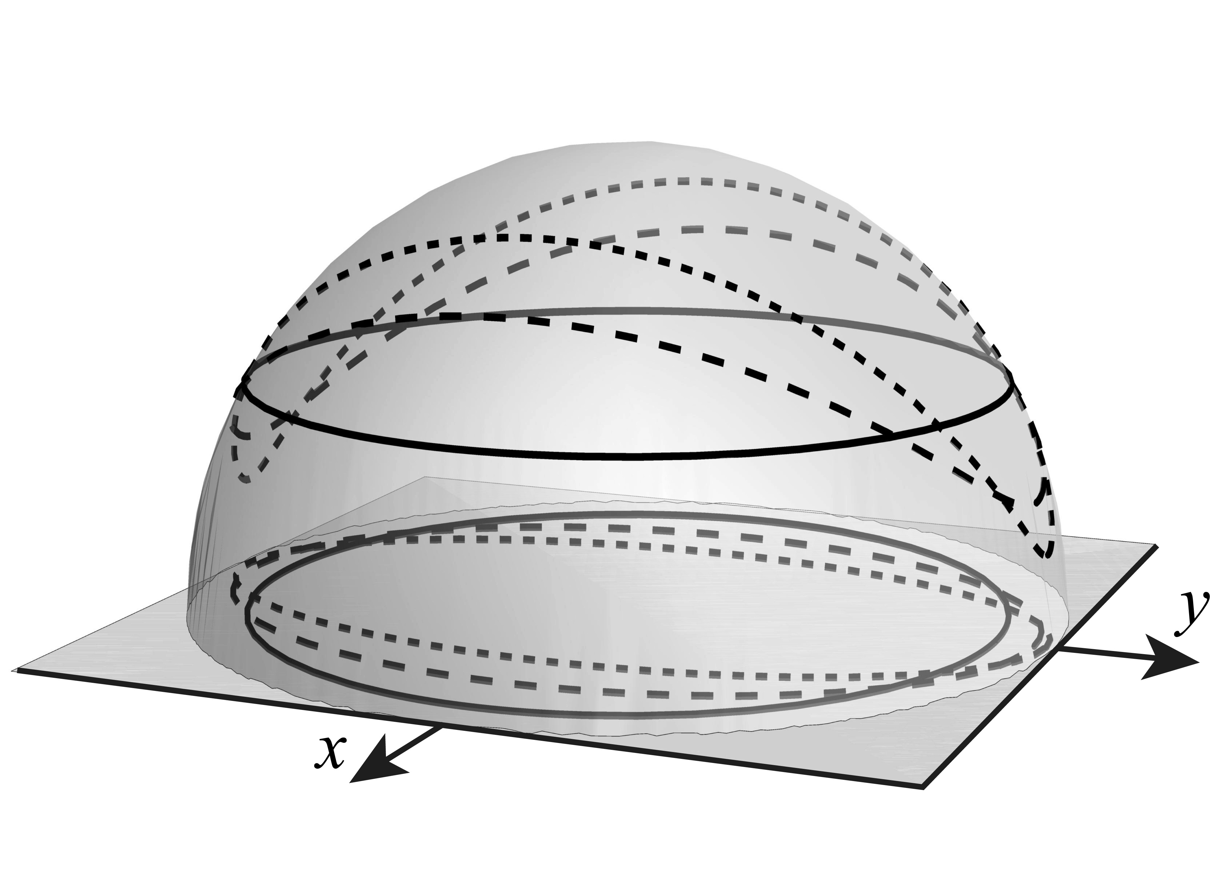
Figure 3: Trajectories $\vartheta(\varphi)$ on the hemisphere given by (52) for the allowed upper regions of the Zernike system $(\alpha_{\scriptscriptstyle\rm Z},\beta_{\scriptscriptstyle\rm Z})=(-1,-2)$ in Fig. 1 (left), and their projection on the $x$–$y$ plane inside the unit disk ${\cal D}_{1}$, for the values corresponding to the upper row of orbits in Fig. 2: $p_{\phi}=3$ and energies $E=15$ (continuous line, the circular orbit at the boundary of the allowed region); $E=20$ (dashed line), and $E=35$ (dotted line).

Still in the $\alpha<0$ case, the pseudo-spherical coordinates ($\tau,\varphi$) of System H^′I in (43) allow separation of the action function as $S(\tau,\varphi)=S_{1}(\tau)+p_{\varphi}\,\varphi$, so the Hamiltonian (37) leads to the equation

$$\alpha\left(\frac{{\rm d}S_{1}}{{\rm d}\tau}\right)^{2}-{\rm i}\beta\coth\tau\,\left(\frac{{\rm d}S_{1}}{{\rm d}\tau}\right)-\frac{\alpha\,p^{2}_{\varphi}}{\cosh^{2}\tau}=E.$$ (53)

Then the trajectories, instead of (52), are given by

$$\cosh^{2}\tau=\frac{|\alpha|\,D}{1-\varepsilon\cos 2\varphi},$$ (54)

with $D$ and $\varepsilon$ given in (23). These are closed orbits in the region $r^{2}>1/|\alpha|$. In Figure 4 we show such trajectories on the one-sheeted half-hyperboloid.

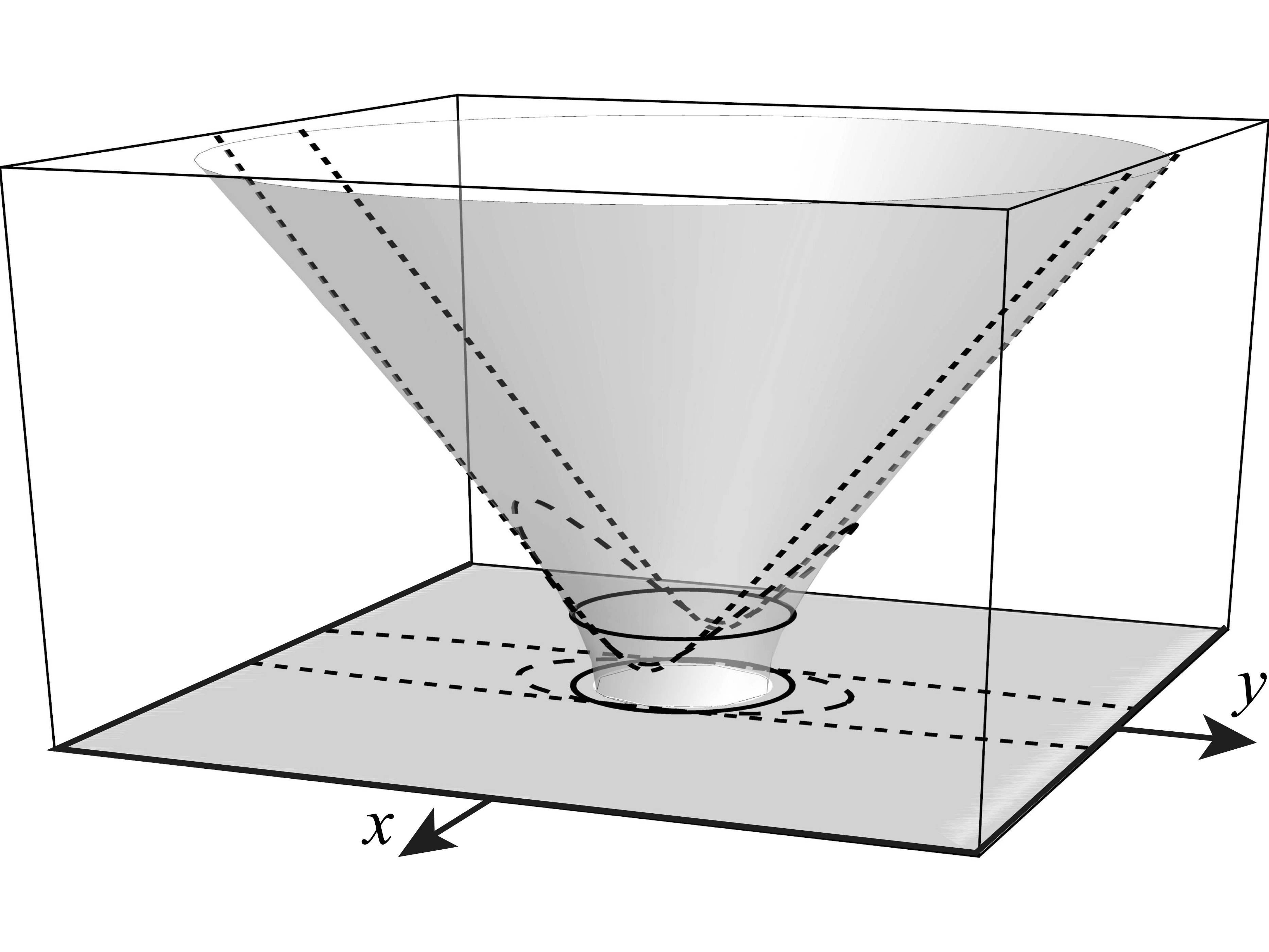
Figure 4: Trajectories $\tau(\varphi)$ on the half-hyperboloid (of one sheet) given by (54), with $\alpha=-1$ and $\beta=-2$, and their projection on the $x$–$y$ plane outside the unit disk ${\cal D}_{1}$. The parameter values are the same as in the second row of Fig. 2, namely $p_{\phi}=3$ and energies $E=3$ (at the upper boundary of the lower allowed region, marked by a continuous line), 1 (dashed line), and $-0.9$ (near to the lower forbidden region, dotted line).

Turning now to the case $\alpha>0$ for the pseudo-spherical system (46), the separation of variables $S(\tau,\varphi)=S_{1}(\tau)+p_{\varphi}\,\varphi$ yields

$$\frac{1+\alpha\varrho^{2}\sinh^{2}\tau}{\varrho^{2}\cosh^{2}\tau}\left(\frac{{\rm d}S_{1}}{{\rm d}\tau}\right)^{2}-{\rm i}\beta\tanh\tau\left(\frac{{\rm d}S_{1}}{{\rm d}\tau}\right)+\frac{p^{2}_{\varphi}}{\varrho^{2}\sinh^{2}\tau}=E,$$ (55)

so that the trajectory $\vartheta(\varphi)$ is found as

$$\sinh^{2}\tau=\frac{\alpha D}{1-\varepsilon\cos 2\varphi},$$ (56)

lying on one sheet of a two-sheeted hyperboloid $\varrho^{2}=1/\alpha$, and where again $D$ and $\varepsilon$ are given in (23). The orbits on this manifold are elliptic and are shown in Fig. 5

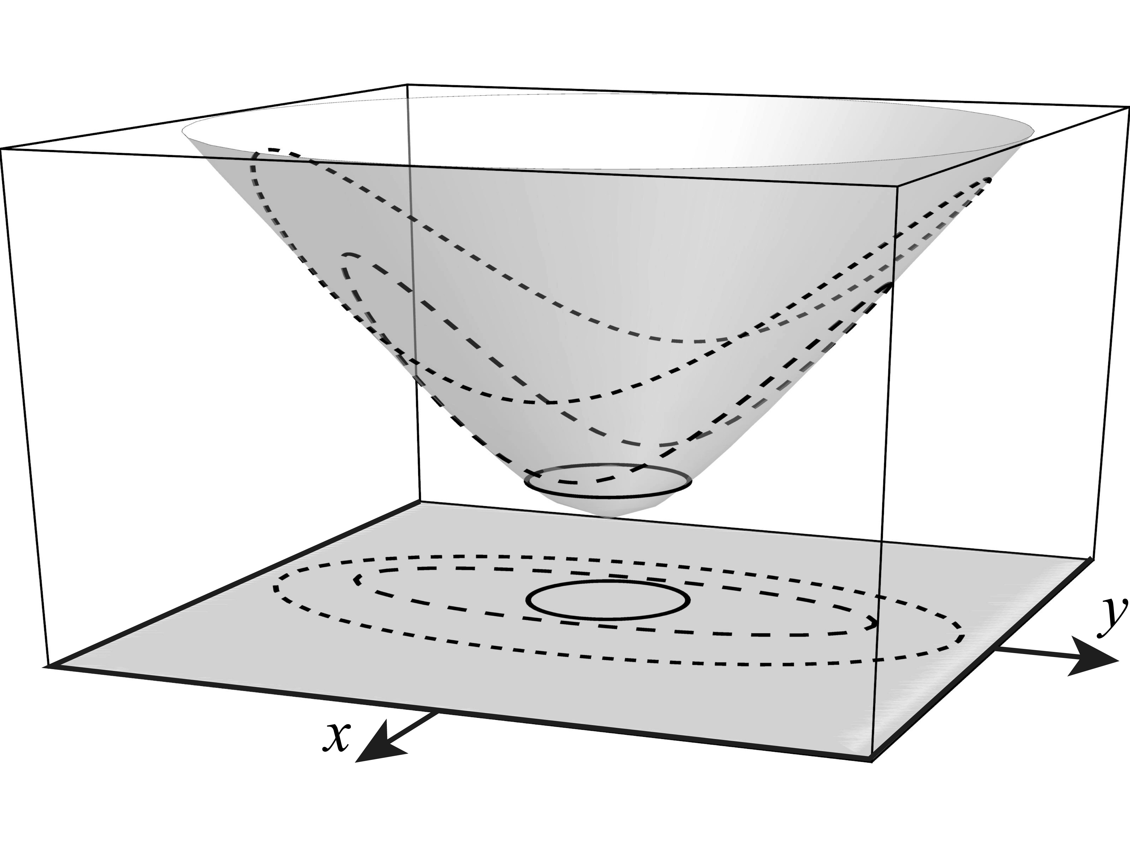
Figure 5: Trajectories $\tau(\varphi)$ on the lower half-hyperboloid (of two sheets) given by (56) with $\alpha=+1$ and $\beta=-2$, and their projection on the full $x$–$y$ plane. The parameter values are all near to the cusp of the allowed region in Fig. 1 (right): $p_{\phi}=0.5$, $E=0.75$ (continuous line); $p_{\phi}=0.75$, $E=0.97$ (dashed line); $p_{\phi}=0.9$, $E=0.993$ (dotted line).

4.3 Separation in coordinate systems II and HII

The second system of spherical coordinates $(\vartheta,\varphi)$ in (41) leads to the Hamiltonian (37) in the form

$$\hskip-30.0pt\frac{1+\alpha R^{2}\cos^{2}\vartheta}{R^{2}\sin^{2}\vartheta}\left(\frac{\partial S}{\partial\vartheta}\right)^{2}+{\rm i}\beta\cot\vartheta\left(\frac{\partial S}{\partial\vartheta}\right)$$

$$\hskip-20.0pt{}+\frac{1}{R^{2}\sin^{2}\vartheta}\left[1+\frac{(1+\alpha R^{2})\cot^{2}\varphi}{\sin^{2}\vartheta}\left(\frac{\partial S}{\partial\varphi}\right)^{2}\right]+{\rm i}\beta\frac{\cot\varphi}{\sin^{2}\vartheta}\left(\frac{\partial S}{\partial\varphi}\right)$$

$$\hskip-20.0pt{}+2\frac{1+\alpha R^{2}}{R^{2}\sin^{2}\vartheta}\cot\vartheta\left(\frac{\partial S}{\partial\vartheta}\right)\cot\varphi\left(\frac{\partial S}{\partial\varphi}\right)=E.$$ (57)

When $\alpha<0$, separation of variables applies on the action function $S(\vartheta,\varphi)=S_{1}(\vartheta)+S_{2}(\varphi)$ and leads to the pair of equations

$$\hskip-20.0pt-\alpha\left(\frac{{\rm d}S_{1}}{{\rm d}\vartheta}\right)^{2}+{\rm i}\beta\cot\vartheta\left(\frac{{\rm d}S_{1}}{{\rm d}\vartheta}\right)+\frac{K_{\scriptscriptstyle\rm II}^{2}}{\sin^{2}\vartheta}=E,$$ (58)

$$\hskip-20.0pt-\alpha\left(\frac{{\rm d}S_{2}}{{\rm d}\varphi}\right)^{2}+{\rm i}\beta\cot\varphi\left(\frac{{\rm d}S_{2}}{{\rm d}\varphi}\right)=K_{\scriptscriptstyle\rm II}^{2},$$ (59)

where $K_{\scriptscriptstyle\rm II}^{2}$ is a separation constant. Rewriting (59) in Cartesian $(x,y)$ coordinates, we obtain

$$\left[1+\alpha(x^{2}+y^{2})\right]\left(\frac{{\rm d}S_{2}}{{\rm d}y}\right)^{2}-{\rm i}\beta\,y\left(\frac{{\rm d}S_{2}}{{\rm d}y}\right)=K_{\scriptscriptstyle\rm II}^{2}.$$ (60)

The integration in $y$ yields a second integral of motion that depends on the parameters $(\alpha,\beta)$,

$$I_{2}:=K_{\scriptscriptstyle\rm II}^{2}=\left[1+\alpha(x^{2}+y^{2})\right]p^{2}_{y}-{\rm i}\beta\,yp_{y}.$$ (61)

In the case $\alpha>0$, the action function admits separation of variables in the hyperbolic equidistant system HII in (44), $S(\tau_{1},\tau_{2})=S_{1}(\tau_{1})+S_{2}(\tau_{2})$ and yields the two equations

$$\hskip-20.0pt\alpha\left(\frac{{\rm d}S_{2}}{{\rm d}\tau_{2}}\right)^{2}-{\rm i}\beta\tanh\tau_{2}\left(\frac{{\rm d}S_{2}}{{\rm d}\tau_{2}}\right)=K_{\scriptscriptstyle\rm HII}^{2},$$ (62)

$$\hskip-20.0pt\alpha\left(\frac{{\rm d}S_{1}}{{\rm d}\tau_{1}}\right)^{2}-{\rm i}\beta\tanh\tau_{1}\left(\frac{{\rm d}S_{1}}{{\rm d}\tau_{1}}\right)+\frac{K_{\scriptscriptstyle\rm HII}^{2}}{\cosh^{2}\tau_{1}}=E,$$ (63)

which lead to the same integral of motion $I_{2}$ in (61).

4.4 Separation in the coordinate system III

The third spherical system of coordinates in (42) leads to the Hamilton-Jacobi form (37) written as

$$\hskip-30.0pt\frac{1+\alpha R^{2}\cos^{2}\vartheta}{R^{2}\sin^{2}\vartheta}\left(\frac{\partial S}{\partial\vartheta}\right)^{2}+{\rm i}\beta\cot\vartheta\left(\frac{\partial S}{\partial\vartheta}\right)$$

$$\hskip-20.0pt{}+\frac{1}{R^{2}\sin^{2}\vartheta}\left[1+\frac{(1+\alpha R^{2})\tan^{2}\varphi}{\sin^{2}\vartheta}\left(\frac{\partial S}{\partial\varphi}\right)^{2}\right]-{\rm i}\beta\frac{\tan\varphi}{\sin^{2}\vartheta}\left(\frac{\partial S}{\partial\varphi}\right)$$

$$\hskip-20.0pt{}-2\frac{1+\alpha R^{2}}{R^{2}\sin^{2}\vartheta}\cot\vartheta\left(\frac{\partial S}{\partial\vartheta}\right)\tan\varphi\left(\frac{\partial S}{\partial\varphi}\right)=E.$$ (64)

In the case $\alpha<0$, for $R^{2}=-1/\alpha$, the separation of variables in the action function, $S(\vartheta,\varphi)=S_{3}(\vartheta)+S_{4}(\varphi)$ leads to

$$\hskip-20.0pt-\alpha\left(\frac{{\rm d}S_{3}}{{\rm d}\vartheta}\right)^{2}+{\rm i}\beta\cot\vartheta\left(\frac{{\rm d}S_{3}}{{\rm d}\vartheta}\right)+\frac{K_{\scriptscriptstyle\rm III}^{2}}{\sin^{2}\vartheta}=E,$$ (65)

$$\hskip-20.0pt-\alpha\left(\frac{{\rm d}S_{4}}{{\rm d}\varphi}\right)^{2}-{\rm i}\beta\tan\varphi\left(\frac{{\rm d}S_{4}}{{\rm d}\varphi}\right)=K_{\scriptscriptstyle\rm III}^{2},$$ (66)

From (66) we find a third constant of motion that depends on $(\alpha,\beta)$,

$$I_{3}:=K_{\scriptscriptstyle\rm III}^{2}=\left[1+\alpha(x^{2}+y^{2})\right]p^{2}_{x}-{\rm i}\beta xp_{x},$$ (67)

and which under the phase space ${\textstyle\frac{1}{2}}\pi$-rotation $(x,p_{x};y,p_{y})\leftrightarrow(y,p_{y};-x,-p_{x})$ coincides with $I_{2}$ in (61). Finally, we note that when $\alpha>0$, the separations of variables (46)–(48) on the hyperboloid yield the same integrals of motion $I_{1}$, $I_{2}$ and $I_{3}$ given above.

We note that, unlike the three orthogonal coordinate systems on the sphere, on hyperboloids there are nine orthogonal coordinate systems where the Laplace and the Helmholtz equations yield to separation of variables [14].

4.5 Separation of variables in the elliptic system

The Hamilton-Jacobi equation (37) also yields to separation in elliptic coordinates on the sphere in trigonometric form [15, 10, 11],

$$\xi^{e}_{1}=R\cos\varphi\sqrt{1{-}k_{1}^{2}\cos^{2}\vartheta},\quad\xi^{e}_{2}=R\sin\vartheta\sin\varphi,\quad\xi^{e}_{3}=R\cos\vartheta\sqrt{1{-}k_{3}^{2}\cos^{2}\varphi},$$ (68)

where the constants $k_{1}:=\cos f$ and $k_{3}:=\sin f$ are related to the interfocal distance $2f$ of the ellipses on the upper unit hemisphere, so that $k_{1}^{2}+k_{3}^{2}=1$. When $\alpha<0$ and thus $R^{2}=1/|\alpha|$, the action function separates as $S(\vartheta,\varphi)=S^{e}_{1}(\vartheta)+S^{e}_{2}(\varphi)$, and leads again to two equations,

$$(1{-}k_{1}^{2}\cos^{2}\vartheta)\left[\alpha\,S_{1}^{e\,\prime\,2}+{\rm i}\beta\tan\vartheta\,S_{1}^{e\,\prime}\right]+Ek_{1}^{2}\sin^{2}\vartheta = K_{e}^{2},$$ (69)

$$\alpha(1{-}k_{3}^{2}\cos^{2}\varphi)S_{2}^{e\,\prime\,2}-{\rm i}\beta k_{3}^{2}\cos\varphi\sin\varphi\,S_{2}^{e\,\prime}+Ek_{3}^{2}\sin^{2}\varphi = -K_{e}^{2},{\quad}$$ (70)

where $K_{e}^{2}$ is a separation constant, $S_{1}^{e\,\prime}:={\rm d}S_{1}/{\rm d}\vartheta$ and $S_{2}^{e\,\prime}:={\rm d}S_{2}/{\rm d}\varphi$. Eliminating $E$ from these equations one obtains

$${\hskip-30.0pt}K_{e}^{2}(k_{3}^{2}\sin^{2}\varphi+k_{1}^{2}\sin^{2}\vartheta)$$

$$= k_{3}^{2}\sin^{2}\varphi(1-k_{1}^{2}\cos^{2}\vartheta)\left[\alpha\left(S^{\prime}_{1}\right)^{2}+{\rm i}\beta\tan\vartheta S^{\prime}_{1}\right]$$

$${}-k_{1}^{2}\sin^{2}\vartheta\left[\alpha(1-k_{3}^{2}\cos^{2}\varphi)\left(S^{\prime}_{2}\right)^{2}-{\rm i}\beta k_{3}^{2}\cos\varphi\sin\varphi S^{\prime}_{2}\right].$$

Returning to Cartesian $(x,y)$ coordinates,

$$\frac{S_{1}^{e\,\prime}}{R} = p_{x}\frac{k_{1}^{2}\sin\vartheta\cos\vartheta\cos\varphi}{\sqrt{1-k_{1}^{2}\cos^{2}\vartheta}}+p_{y}\cos\vartheta\sin\varphi,$$ (72)

$$\frac{S_{2}^{e\,\prime}}{R} = -p_{x}\sqrt{1-k_{1}^{2}\cos^{2}\vartheta}\,\sin\varphi+p_{y}\sin\vartheta\cos\varphi,$$ (73)

we can express the constant $K_{e}^{2}$ as

$$\begin{array}[]{rcl}K_{e}^{2}&=&-\alpha k_{1}^{2}y^{2}p_{x}^{2}+2\alpha k_{1}^{2}xyp_{x}p_{y}\\[3.0pt] &&\displaystyle{\!}-\Big{(}\alpha k_{1}^{2}x^{2}+k_{3}^{2}[1+\alpha(x^{2}+y^{2})]\Big{)}p^{2}_{y}+{\rm i}\beta k_{3}^{2}yp_{y}\\[3.0pt] &=&-\alpha k_{1}^{2}I_{1}^{2}-k_{3}^{2}I_{2}.\end{array}$$ (74)

Thus the elliptic separation constant $K_{e}^{2}$ is not functionally independent but depends on the constants $I_{1}$ and $I_{2}$ in (50) and (61).

5 Algebraic structure and conclusions

We have found three functionally independent integrals of motion, $I_{1}$ in (50), $I_{2}$ in (61), and $I_{3}$ in (67) with no singularities on the full $(\alpha,\beta)$ parameter space. To probe their algebraic structure let us define

$$J_{1} := {\textstyle\frac{1}{2}}I_{1}={\textstyle\frac{1}{2}}(xp_{y}-yp_{x}),$$ (75)

$$J_{2} := {\textstyle\frac{1}{2}}(I_{3}-I_{2})={\textstyle\frac{1}{2}}\left[1+\alpha(x^{2}+y^{2})\right](p^{2}_{x}-p_{y}^{2})-{\textstyle\frac{1}{2}}{\rm i}\beta(xp_{x}-yp_{y}).{\qquad}$$ (76)

The function $J_{1}$ is ${\textstyle\frac{1}{2}}$-angular momentum and its Poisson operator $\{J_{1},\circ\}$ generates rotations of phase space, while the function $J_{2}$ does depend on $(\alpha,\beta)$. These functions Poisson-commute with the Zernike Hamiltonian function $H^{(\alpha,\beta)}$ in (4), which can be written as

$$H^{(\alpha,\beta)}=I_{3}+I_{2}-\alpha I_{1}^{2},$$ (77)

but do not commute with each other. This shows that the generalized classical $(\alpha,\beta)$-Hamiltonian of Zernike, $H^{(\alpha,\beta)}$ in (5), is superintegrable on each of the domains examined above, in particular on the $(x,y)$-disk ${\cal D}_{\scriptscriptstyle\rm R}$, $r<R=1/\surd|\alpha|$ for $\alpha<0$, that contains the Zernike original case $(\alpha_{\scriptscriptstyle\rm Z},\beta_{\scriptscriptstyle\rm Z})=(-1,-2)$.

To identify the symmetry of the generalized Zernike $(\alpha,\beta)$-Hamiltonians, we introduce a new integral of motion through the Poisson bracket of (75) and (76),

$$J_{3}:=\{J_{1},J_{2}\}=\left[1+\alpha(x^{2}+y^{2})\right]p_{x}p_{y}-{\rm i}{\textstyle\frac{1}{2}}\beta(xp_{y}+yp_{x}),$$ (78)

which also Poisson-commutes with $H^{(\alpha,\beta)}$, and is functionally independent of $J_{1}$ and $J_{2}$, although it can be seen that $J_{2}$ and $J_{3}$ are connected to each other by a rotation of $\frac{1}{4}\pi$ in the $x$–$y$ phase space planes. The algebraic structure of three functions $J_{1},\,J_{2},\,J_{3}$ is thus found to be

$$\{J_{3},J_{1}\} = J_{2},\qquad\{J_{1},J_{2}\}=J_{3},$$ (79)

$$\{J_{2},J_{3}\} = J_{1}(\beta^{2}-2\alpha H^{(\alpha,\beta)}-8\alpha^{2}J_{1}^{2}).$$ (80)

They form therefore a cubic Higgs algebra [7] that Poisson-commutes with the generalized Zernike Hamiltonian, $\{J_{i},H^{(\alpha,\beta)}\}=0$.

When $\alpha\to 0$ so $R\to\infty$, the Zernike Hamiltonian becomes a simpler quadratic function,

$$H^{(0,\beta)}({\bf q},{\bf p})={\bf p}^{2}-{\rm i}\beta\,{\bf q}\cdot{\bf p}.$$ (81)

The Poisson operators of all quadratic functions of these four phase space coordinates close under commutation into the real symplectic Lie algebra sp($4$,R).

The Hamiltonian (81) belongs to the elliptic orbit of harmonic oscillators [21, Chap. 12], as can be seen under the complex linear canonical transformation

$$\left(\matrix{\displaystyle{{\bf p}}{}_{\mathstrut}\cr\displaystyle{{\bf q}}\cr}\right)=\left(\matrix{\displaystyle{{\bf 1}/\surd 2}&\displaystyle{{\rm i}\beta{\bf 1}/\surd 2}{}_{\mathstrut}\cr\displaystyle{{\bf 0}}&\displaystyle{\surd 2\,{\bf 1}}\cr}\right)\left(\matrix{\displaystyle{{\bf P}}{}_{\mathstrut}\cr\displaystyle{{\bf Q}}\cr}\right).$$ (82)

This maps (81) on a regular harmonic oscillator,

$$F_{0}:=H^{(0,\beta)}({\bf Q},{\bf P})={\textstyle\frac{1}{2}}({\bf P}^{2}+\beta^{2}{\bf Q}^{2}),$$ (83)

and the three constants of the motion, $J_{1},\,J_{2},\,J_{3}$ in (75), (76) and (78), on

$$F_{1} := {\textstyle\frac{1}{2}}\,{\bf Q}\times{\bf P}={\textstyle\frac{1}{2}}(Q_{x}P_{y}-Q_{y}P_{x}),$$ (84)

$$F_{2} := {\textstyle\frac{1}{2}}(P_{x}^{2}+\beta Q_{x}^{2})-{\textstyle\frac{1}{2}}(P_{y}^{2}+\beta^{2}Q_{y}^{2}),$$ (85)

$$F_{3} := {\textstyle\frac{1}{2}}P_{x}P_{y}+{\textstyle\frac{1}{2}}\beta^{2}\,Q_{x}Q_{y}$$ (86)

whose Poisson brackets close into a scaled u($2$) Lie algebra,

$$\{F_{1},F_{2}\}=F_{3},\quad\{F_{2},F_{3}\}=\beta^{2}F_{1},\quad\{F_{3},F_{1}\}=F_{2},\quad\ \{F_{0},F_{i}\}=0.$$ (87)

In the paraxial geometric or wave optical interpretation, the central $F_{0}\in{\sf u({\rm 1})}$ generates isotropic fractional Fourier transforms [19], while $F_{2}$ generates anisotropic ones, $F_{1}$ generates rotations, and $F_{3}$ generates gyrations [17] that transform Hermite-Gauss into Laguerre-Gauss beams. Together their Poisson operators form the Fourier algebra [19], which is the maximal compact subalgebra in sp($4$,R). If $\beta$ were a pure imaginary number, (83) would be the repulsive oscillator Hamiltonian and (84)–(86) its commuting ‘Fourier’ algebra ${\sf su({\rm 1,1})}={\sf so({\rm 2,1})}$; a similar treatment of the classical system with Hamiltonian (4) would yield hyperbolic orbits. For $\beta=0$ a free system with an inhomogeneous iso(2) ‘Fourier’ algebra would appear.

The original Zernike system $\hat{Z}^{(\alpha_{\scriptscriptstyle\rm Z},\beta_{\scriptscriptstyle\rm Z})}$ in (1) [23] was proposed to develop a set orthogonal and complete set of two-variable orthogonal polynomials $Z_{n,m}(r)\exp({\rm i}m\phi)$, $Z_{n,m}(1)=1$, $|m|\leq n$, which present the same $(n,m)$-pattern as the two-dimensional quantum harmonic oscillator states. There has been some effort in replicating the raising and lowering techniques of the oscillator scheme on the Zernike system [22, 18] without achieving a proper Lie algebra. Because here we have a two-parameter system $H^{(\alpha,\beta)}$, we could surmise that superintegrable systems can be obtained as a new kind of algebra deformation, from (83)–(87) to (75)–(80), consisting in the addition of the square of an element of a Lie algebra to the generator designed to be the original quadratic Hamiltonian. Imposing boundary conditions such as those proposed by Zernike will need the quantum treatment of this construction.

References

[1] J. Bertrand, Théorème relatif au mouvement d’un
point attiré vers un centre fixe, C. R. Acad. Sci.77, 849–853 (1873).
[2] A. B. Bhatia and E. Wolf, On the circle polynomials
of Zernike and related orthogonal sets, Math. Proc. Cambridge Phil. Soc.50, 40–48 (1954).
[3] M. Born and E. Wolf, Principles of Optics:
Electromagnetic Theory of Propagation, Interference and Diffraction
of Light 7th ed. (Cambridge University Press, 1999). p. 986.
[4] J. F. Cariñena, M. F. Rañada and M. Santander,
Two important examples of nonlinear oscillators, arXiv:math-ph/0505028.
[5] J. F. Cariñena, A. M. Perelomov and M. F. Rañada,
Isochronous classical systems and quantum systems with equally
spaced spectra, J. Phys.: Conf. Ser.87, 012007, 4 p. (2007).
[6] I. S. Gradshteyn and I. M. Ryzhik, Table of Integrals,
Series, and Products (6th Ed., Academic Press, 2000).
[7] P. W. Higgs, Dynamical symmetries in a spherical geometry,
J. Phys. A12, 309–323 (1979).
[8] M. E. H. Ismail and R. Zhang, Classes of bivariate
orthogonal polynomials, SIGMA12, 021 (2016),
arXiv:1502.07256v3 [math.CA].
[9] E. C. Kintner, On the mathematical properties
of the Zernike Polynomials, Opt. Acta23, 679–680 (1976).
[10] I. Lukac and Ya. A. Smorodinskiĭ, Wave functions
for the asymmetric top, Sov. Phys. JETP30, 728–730 (1970).
[11] I. Lukach, A complete set of the quantum-mechanical
observables on a two-dimensional sphere, Theor. Math. Phys.14, 271–281 (1973).
[12] W. Miller Jr., S. Post, P. Winternitz, Classical
and quantum superintegrability with applications, J. Phys. A47, 423001, 97 p. (2014).
[13] D. R. Myrick, A Generalization of the radial polynomials
of F. Zernike, SIAM J. Appl. Math.14, 476–489 (1966).
[14] M. N. Olevskiĭ, Triorthogonal systems in
spaces of constant curvature in which the equation allows a complete separation of variables,
Mat. Sbornik27, 379–426 (1950).
[15] G. S. Pogosyan, A. N. Sissakian and P. Winternitz,
Separation of variables and Lie algebra contractions. Applications
to special functions, Phys. Part. Nuclei33, Suppl. 1, S123–S144 (2002).
[16] G. S. Pogosyan and A. Yakhno, Lie algebra
contractions and separation of variables on two-dimensional
hyperboloidal coordinate systems. ArXiv 1510.03785 V1 (2015).
[17] J. A. Rodrigo, T. Alieva and T. J. Bastiaans
Phase space rotators and their applications in optics. In: Optical and Digital Image Processing: Fundamentals and Applications,
pp. 251–271. G. Cristóbal, P. Schelkens and H. Thienpont Eds.
(Wiley-VCH Verlag, 2011).
[18] B. H. Shakibaei and R. Paramesran, Recursive
formula to compute Zernike radial polynomials,
Opt. Lett.38, 2487–2489 (2013).
[19] R. Simon and K. B. Wolf, Structure of the set
of paraxial optical systems. J. Opt. Soc. Am. A17, 342–355 (2000).
[20] W. J. Tango, The circle polynomials of Zernike
and their application in optics, Appl. Phys.13, 327–332 (1977).
[21] K. B. Wolf, Geometric Optics on Phase Space
(Springer, Heidelberg, 2004).
[22] A. Wünsche, Generalized Zernike or disc polynomials,
J. Comp. App. Math.174, 135–163 (2005).
[23] F. Zernike, Beugungstheorie des Schneidenverfahrens
und Seiner Verbesserten Form der Phasenkontrastmethode,
Physica1, 689–704 (1934).