Nearly Maximally Predictive Features and Their Dimensions

Abstract

Scientific explanation often requires inferring maximally predictive features from a given data set. Unfortunately, the collection of minimal maximally predictive features for most stochastic processes is uncountably infinite. In such cases, one compromises and instead seeks nearly maximally predictive features. Here, we derive upper-bounds on the rates at which the number and the coding cost of nearly maximally predictive features scales with desired predictive power. The rates are determined by the fractal dimensions of a process’ mixed-state distribution. These results, in turn, show how widely-used finite-order Markov models can fail as predictors and that mixed-state predictive features offer a substantial improvement.

Often, we wish to find a minimal maximally predictive model consistent with available data. Perhaps we are designing interactive agents that reap greater rewards by developing a predictive model of their environment [1, 2, 3, 4, 5, 6] or, perhaps, we wish to build a predictive model of experimental data because we believe that the resultant model gives insight into the underlying mechanisms of the system [7, 8]. Either way, we are almost always faced with constraints that force us to efficiently compress our data [9].

Ideally, we would compress information about the past without sacrificing any predictive power. For stochastic processes generated by finite unifilar hidden Markov models (HMMs), one need only store a finite number of predictive features. The minimal such features are called causal states, their coding cost is the statistical complexity $C_{\mu}$ [10], and the implied unifilar HMM is the $\epsilon$-machine [10, 11]. However, most processes require an infinite number of causal states [7] and so cannot be described by finite unifilar HMMs.

In these cases, we can only attain some maximal level of predictive power given constraints on the number of predictive features or their coding cost. Equivalently, from finite data we can only infer a finite predictive model. Thus, we need to know how our predictive power grows with available resources.

Recent work elucidated the tradeoffs between resource constraints and predictive power for stochastic processes generated by countable unifilar HMMs or, equivalently, described by a finite or countably infinite number of causal states [12, 13, 14]. Few, though, studied this tradeoff or provided bounds thereof more generally.

Here, we place new bounds on resource-prediction tradeoffs in the limit of nearly maximal predictive power for processes with either a countable or an uncountable infinity of causal states by coarse-graining the mixed-state simplex [15]. These bounds give a novel operational interpretation to the fractal dimension of the mixed-state simplex and suggest new routes towards quantifying the memory stored in a stochastic process when, as is typical, statistical complexity diverges.

Background

We consider a discrete-time, discrete-state stochastic process $\mathcal{P}$ generated by an HMM $\mathcal{G}$, which comes equipped with underlying states $g$ and labeled transition matrices $T^{{x}}_{g,g^{\prime}}=\Pr(\mathcal{G}_{t+1}=g^{\prime},{X}_{t+1}={x}|\mathcal{G}_{t}=g)$ [16]. There is an infinite number of alternate HMMs that generate $\mathcal{P}$ [17, 18, 19, 20], so we specify here that $\mathcal{G}$ is the minimal generative model—that is, the generative model with the minimal number of hidden states consistent with the observed process .

For reasons that become clear shortly, we are interested in the block entropy $\operatorname{H}(L)=\operatorname{H}[{X}_{0:L}]$, where ${X}_{a:b}={X}_{a},{X}_{a+1},\ldots,{X}_{b-1}$ is a contiguous block of random variables generated by $\mathcal{G}$. In particular, its growth—the entropy rate $h_{\mu}=\lim_{L\rightarrow\infty}\operatorname{H}(L)/L$—quantifies a process’ intrinsic “randomness”. While the excess entropy ${\bf E}=\lim_{L\rightarrow\infty}\left(\operatorname{H}(L)-h_{\mu}L\right)$ quantifies how much is predictable: how much future information can be predicted from the past . Finite-length entropy-rate estimates $h_{\mu}(L)=\operatorname{H}[{X}_{0}|{X}_{-L:0}]$ provide increasingly better approximations to the true entropy rate $h_{\mu}$ as $L$ grows large. While finite-length excess-entropy estimates:

$${\bf E}(L) =\operatorname{H}(L)-h_{\mu}L$$ (1)

$$=\sum_{\ell=0}^{L-1}\left(h_{\mu}(\ell)-h_{\mu}\right)~{}.$$ (2)

tend to the true excess entropy ${\bf E}$ as $L$ grows large [23]. As there, we consider only finitary processes, those with finite ${\bf E}$ .

Predictive features $\mathcal{R}$ from some alphabet $\mathcal{F}$ are formed by compressing the process’ past ${X}_{-\infty:0}$ in ways that implicitly retain information about the future ${X}_{0:\infty}$. (From hereon, our block notation suppresses infinite indices.) A predictive distortion quantifies the predictability lost after such a coarse-graining:

$$d(\mathcal{R}) =\operatorname{I}[{X}_{:0};{X}_{0:}|\mathcal{R}]$$

$$={\bf E}-\operatorname{I}[\mathcal{R};{X}_{0:}]~{}.$$

On the one hand, distortion achieves its maximum value ${\bf E}$ when $\mathcal{R}$ captures no information from the past that could be used for prediction. On the other, it can be made to vanish trivially by taking the predictive features $\mathcal{R}$ to be all of the possible histories ${X}_{:0}$. Here, we quantify the cost of a larger feature space in two ways: by the number $|\mathcal{F}|$ of predictive features and by their coding cost $H[\mathcal{R}]$ [25].

Results

Ideally, we would identify the minimal number $|\mathcal{F}|$ of predictive features or the coding cost $H[\mathcal{R}]$ required to achieve at least a given level $d$ of predictive distortion. This is almost always a difficult optimization problem. However, we can place upper bounds on $|\mathcal{F}|$ and $H[\mathcal{R}]$ by constructing suboptimal predictive feature sets that achieve predictive distortion $d$.

We start by reminding ourselves of the optimal solution in the limit that $d=0$—the causal states $\mathcal{S}$ [10, 11, 13]. Causal states can be defined by calling two pasts, ${x}_{:0}$ and ${x}_{:0}^{\prime}$, equivalent when using them our predictions of the future are the same: $\Pr({X}_{0:}|{X}_{:0}={x}_{:0})=\Pr({X}_{0:}|{X}_{:0}={x}_{:0}^{\prime})$. (These conditional distributions are referred to as future morphs.) One can then form a model, the $\epsilon$-machine, from the set $\mathcal{S}$ of causal-state equivalence classes and their transition operators. The Shannon entropy of the causal state distribution is the statistical complexity: $C_{\mu}=\operatorname{H}[\mathcal{S}]$. A process’ $\epsilon$-machine can also be viewed as the minimal unifilar HMM capable of generating the process [26] and $C_{\mu}$ the amount of historical information the process stores in its causal states. Though the mechanics of working with causal states can become rather sophisticated, the essential idea is that causal states are designed to capture everything about the past relevant to predicting the future and only that information.

In the lossless limit, when $d=0$, one cannot find predictive representations that achieve $|\mathcal{F}|$ smaller than $|\mathcal{S}|$ or that achieve $\operatorname{H}[\mathcal{R}]$ smaller than $C_{\mu}$. Similarly, no optimal lossy predictive representation will ever find $|\mathcal{F}|>|\mathcal{S}|$ or $\operatorname{H}[\mathcal{R}]\geq C_{\mu}$. When the number of causal states is infinite or statistical complexity diverges, as is typical, as we noted, these bounds are quite useless; but otherwise, they provide a useful calibration for the feature sets proposed below.

Markov Features

Several familiar predictive models use pasts of length $L$ as predictive features. This feature set can be thought of as constructing an order-$L$ Markov model of a process . The implied predictive distortion is $d(L)=\operatorname{I}[{X}_{:0};{X}_{0:}|{X}_{0:L}]={\bf E}-{\bf E}(L)$ [28], while the number of features is the number of length-$L$ words with nonzero probability and their entropy $\operatorname{H}[\mathcal{R}]=\operatorname{H}(L)$. Generally, $h_{\mu}(L)$ converges exponentially quickly to the true entropy rate $h_{\mu}$ for stochastic processes generated by finite-state HMMs, unifilar or not; see Ref. [29] and references therein. Then, $h_{\mu}(L)-h_{\mu}\sim Ke^{-\lambda L}$ in the large $L$ limit. From Eq. (2), we see that the convergence rate $\lambda$ also implies an exponential rate of decay for ${\bf E}-{\bf E}(L)\sim K^{\prime}e^{-\lambda L}$. Additionally, according to the asymptotic equipartition property [25], when $L$ is large, $|\mathcal{F}|\sim e^{h_{0}L}$ and $\operatorname{H}(L)\approx h_{\mu}L$, where $h_{0}$ is the topological entropy and $h_{\mu}$ the entropy rate, both in nats.

In sum, this first set of predictive features—effectively, the construction of order-$L$ Markov models—yields an algebraic tradeoff between the size of the feature set $\mathcal{F}$ and the predictive distortion $d$:

$$|\mathcal{F}|\sim\left(\frac{1}{d}\right)^{h_{0}/\lambda},$$ (3)

and a logarithmic tradeoff between the entropy of the features and distortion:

$$H[\mathcal{R}]\sim\frac{h_{\mu}}{\lambda}\log\left(\frac{1}{d}\right)~{}.$$ (4)

In principle, $\lambda$ can be arbitrarily small, and so $h_{0}/\lambda$ and $h_{\mu}/\lambda$ arbitrarily large, even for processes generated by finite-state HMMs. This can be true even for finite unifilar HMMs ($\epsilon$-machines). To see this, let $W$ be the transition matrix of a process’ mixed-state presentation; defined shortly. From Ref. [28], when $W$’s spectral gap $\gamma$ is small, we have ${\bf E}-{\bf E}(L)\sim(1-\gamma)^{L}$, so that $\lambda=\log\frac{1}{1-\gamma}$ can be quite small.

In short, when the process in question has only a finite number of causal states, $|\mathcal{F}|$ optimally saturates at $|\mathcal{S}|$ and $H[\mathcal{R}]$ optimally saturates at $C_{\mu}$, but from Eqs. (3) and (4), the size of this Markov feature set can grow without bound when we attempt to achieve zero predictive distortion.

Mixed-State Features

A different predictive feature set comes from coarse-graining the mixed-state simplex. As first described by Blackwell [15], mixed states $Y$ are probability distributions $\Pr(\mathcal{G}_{0}|{X}_{-L:0}={x}_{-L:0})$ over the internal states $\mathcal{G}$ of a generative model given the generated sequences. Transient mixed states are those at finite $L$, while recurrent mixed states are those remaining with positive probability in the limit that $L\to\infty$. Recurrent mixed states exactly correspond to causal states $\mathcal{S}$ [30]. When $C_{\mu}$ diverges, recurrent mixed states often lay on a Cantor set in the simplex; see Fig. 1. In this circumstance, one examines the various dimensions that describe the scaling in such sets. Here, for reasons that will become clear, we use the box-counting $\text{dim}_{0}(Y)$ and information dimensions $\text{dim}_{1}(Y)$ [31].

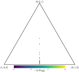
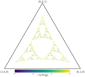
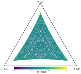
Figure 1: Mixed state presentations $Y$ for three different generative models given in Supplementary Materials App. A. To visualize the mixed-state simplex, the diagrams plot iterates $y_{t}$ such that the left vertex corresponds to the pure state $\Pr(A,B,C)=(1,0,0)$ or HMM state $A$, the right to pure state $(0,1,0)$ or HMM state $B$, and the top to pure state $(0,0,1)$ or HMM state $C$. Left plot has $55$ mixed states plotted in a $1\times 100$ bin histogram; middle plots $2,391,484$ mixed states in a $1000\times 1000$ bin histogram; and right plots $21,523,360$ mixed states in a $4000\times 4000$ bin histogram. Bin cell coloring is negative logarithm of the normalized bin counts. The box-counting dimensions are respectively: $\text{dim}_{0}(Y)\approx 0.3$ at left, $\text{dim}_{0}(Y)\approx 1.8$ in the middle, and $\text{dim}_{0}(Y)\approx 1.9$ at right. Box-counting dimension calculated by estimating the slope of $\log(1/\epsilon)$ versus $\log N_{\epsilon}$ as described in Supplementary Materials App. A.

More concretely, we partition the simplex into cubes of side length $\epsilon$, and each nonempty cube is taken to be a predictive feature in our representation. When there are only a finite number of causal states, then this feature set consists of the causal states $\mathcal{S}$ for some nonzero $\epsilon$. There is no such $\epsilon$ if, instead, the process has a countable infinity of causal states. Sometimes, as for the finite $|\mathcal{S}|$ case, the information dimension and perhaps even the box-counting dimension of the mixed states will vanish. When there is an uncountable infinity of causal states and $\epsilon$ is sufficiently small, the corresponding number of features scales as:

$$|\mathcal{F}|\sim\left(\frac{1}{\epsilon}\right)^{\text{dim}_{0}(Y)}~{},$$

where $\text{dim}_{0}(Y)$ denotes the box-counting dimension and the coding cost scales as:

$$\operatorname{H}[\mathcal{R}]\sim\text{dim}_{1}(Y)\log\frac{1}{\epsilon}~{},$$

where $\text{dim}_{1}(Y)$ is the information dimension. These dimensions can be approximated numerically; see Fig. 1 and Supplementary Materials App. A.

For processes generated by infinite $\epsilon$-machines, finding the better feature set requires analyzing the scaling of predictive distortion with $\epsilon$. Supplementary Materials App. B shows that $d(\mathcal{R})$ at coarse-graining $\epsilon$ scales at most as $\epsilon$ in the limit of asymptotically small $\epsilon$. Our upper bound relies on the fact that two nearby mixed states have similar future morphs, i.e., they have similar conditional probability distributions over future trajectories given one’s mixed state. From this, we conclude that:

$$|\mathcal{F}|\sim\left(\frac{1}{d}\right)^{\text{dim}_{0}(Y)}$$ (5)

and

$$\operatorname{H}[\mathcal{R}]\sim\text{dim}_{1}(Y)\log\frac{1}{d}~{}.$$ (6)

In general, both $\text{dim}_{0}(Y)$ and $\text{dim}_{1}(Y)$ are bounded above by $|\mathcal{G}|$, the number of states in the minimal generative model.

Resource-Prediction Tradeoff

Finally, putting Eqs. (3)-(6) together, we find that for a process with an uncountably infinite $\epsilon$-machine, the necessary number of predictive features $|\mathcal{F}^{*}|$ scales no faster than:

$$|\mathcal{F}^{*}|\lesssim\left(\frac{1}{d}\right)^{\min(h_{0}/\lambda,\text{dim}_{0}(Y))}$$ (7)

and the requisite coding cost $\operatorname{H}[\mathcal{R}^{*}]$ scales no faster than:

$$\operatorname{H}[\mathcal{R}^{*}]\lesssim\min(h_{\mu}/\lambda,\text{dim}_{1}(Y))\log\frac{1}{d}~{},$$ (8)

where $d$ is predictive distortion.

These bounds have a practical interpretation. From finite data, one can only justify inferring finite-state minimal maximally predictive models. Indeed, the criteria of Ref. [33] applied as in Ref. [13] suggests that the maximum number of inferred states should not yield predictive distortions below the noise in our estimate of predictive distortion $d$ from $T$ data points. This noise scales as $\sim 1/\sqrt{T}$, since from $T$ data points, we have approximately $T$ separate measurements of predictive distortion. This, in turn, sets upper bounds on $|\mathcal{F}^{*}|\lesssim T^{\frac{1}{2}\min(h_{0}/\lambda,\text{dim}_{0}(Y))}$ and $\operatorname{H}[\mathcal{R}^{*}]\lesssim\min(h_{\mu}/\lambda,\text{dim}_{1}(Y))\log T$ when the process in question has an uncountable infinity of causal states.

We can test this prediction directly using the Bayesian Structural Inference (BSI) algorithm [34] applied to the processes described in Fig. 1. The major difficulty in employing BSI is that one must specify a list of $\epsilon$-machine topologies to search over. Since the number of such topologies grows super-exponentially with the number of states [35], experimentally probing the scaling behavior of the number of inferred states with the amount of available data is, with nothing else said, impossible.

However, “expert knowledge” can cull the number of $\epsilon$-machine topologies that one should search over. In this spirit, we focus on the Simple Nonunifilar Source (SNS), since $\epsilon$-machines for renewal processes have been characterized in detail [36, 37, 38, 39]. The SNS’s generative HMM is given in Fig. 2(left). This process has a mixed-state presentation similar to that of “nond” in Fig. 1(left). We choose to only search over the $\epsilon$-machine topologies that correspond to the class of eventually Poisson renewal processes.

We must first revisit the upper bound in Eq. (7), as the SNS has a countable (not uncountable) infinity of causal states. When a process’ $\epsilon$-machine is countable instead of uncountable, then we can improve upon Eq. (7). However, the magnitude of improvement is process dependent and not easily characterized in general for two main reasons. First, predictive distortion can decrease faster than $\epsilon$ for processes generated by countably infinite $\epsilon$-machines since there might only be one mixed state in an $\epsilon$ hypercube. (See the lefthand factor in Supplementary Materials Eq. (13), $\sum_{r\in\mathcal{R}^{(\epsilon)}:\operatorname{H}[Y|\mathcal{R}^{(\epsilon)}=r]=0}\pi(r)$. We are guaranteed that $\lim_{\epsilon\rightarrow 0}\sum_{r\in\mathcal{R}^{(\epsilon)}:\operatorname{H}[Y|\mathcal{R}^{(\epsilon)}=r]=0}\pi(r)=0$, but the rate of convergence to zero is highly process dependent.) Second, the scaling relation between $N_{\epsilon}$ and $1/\epsilon$ may be subpower law.

Figure 2: Model-size scaling for the parametrized Simple Nonunifilar Source (SNS). (Top) Generative HMM for the SNS. (Bottom) Scaling of $\langle|M|\rangle=\sum_{M}|M|P(M|x_{0:T})$ with $T$, with the posterior $P(M|x_{0:T})$ calculated using formulae from BSI [34] with $\alpha=1$ and the set of model topologies being the eventually Poisson $\epsilon$-machines described in Ref. [36]. Data generated from the SNS with $p=q=\frac{1}{2}$. Linear regression reveals a slope of $\approx 1$ for $\log\log T$ vs. $\log\langle|M|\rangle$, confirming the expected $N_{T}\begin{subarray}{l}\propto\\[-2.0pt] \sim\end{subarray}\log T$, where the proportionality constants depend on $\beta$.

Given a specific process, though, with a countably infinite $\epsilon$-machine—here, the SNS—we can derive expected scaling relations. See Supplementary Materials App. C. We argue that, roughly speaking, we should expect predictive distortion to decay exponentially with $N_{\epsilon}$, so that $d(\mathcal{R}_{\epsilon})~{}\begin{subarray}{l}\propto\\[-2.0pt] \sim\end{subarray}~{}\lambda^{N_{\epsilon}}$ for some $\lambda<1$. As we expect, since our uncertainty in $d$ scales as $\sim 1/\sqrt{T}$, where $T$ is the amount of data, we expect that the number of inferred states $N_{T}$ should scale as $\begin{subarray}{l}\propto\\[-2.0pt] \sim\end{subarray}~{}\log T$.

These scaling relationships are confirmed by BSI applied to data generated from the SNS, where the set of $\epsilon$-machine topologies selected from are the eventually Poisson $\epsilon$-machine topologies characterized by Ref. [36]. Given a set of machines $\mathcal{M}$ and data $x_{0:T}$, BSI returns an easily-calculable posterior $\Pr(M|x_{0:T})$ for $M\in\mathcal{M}$ with (at least) two hyperparameters: (i) the concentration parameter for our Dirichlet prior on the transition probabilities $\alpha$ and (ii) our prior on the likelihood of a model $M$ with number of states $|M|$, taken to be proportional to $e^{-\beta|M|}$ for a user-specified $\beta$. From this posterior, we calculate an average model size $\langle|M|\rangle(T)=\sum_{M\in\mathcal{M}}|M|\Pr(M|x_{0:T})$ as a function of $T$ for multiple data strings $x_{0:T}$. The result is that we find the exact scaling of $\langle|M|\rangle(T)$ with $T$ is proportional to $\log T$ in the large $T$ limit, where the proportionality constant and the initial value depends on hyperparameters $\alpha$ and $\beta$.

Conclusion

We now better understand the tradeoff between memory and prediction in processes generated by a finite-state Hidden Markov model with infinite statistical complexity. Importantly and perhaps still underappreciated, these processes are more “typical” than those with finite statistical complexity and Gaussian processes, which have received more attention in related literature [12, 13].

We proposed a new method for obtaining predictive features—coarse-graining mixed states—and used this feature set to bound the number of features and their coding cost in the limit of small predictive distortion. These bounds were compared to those obtained from the more familiar and widely used (Markov) predictive feature set—that of memorizing all pasts of a fixed length. The general results here suggest that the new feature set can outperform the standard set in many situations.

Practically speaking, the new bounds presented have three potential uses. First, they give weight to Ref. [7]’s suggestion to replace the statistical complexity with the information dimension of mixed-state space as a complexity measure when statistical complexity diverges. Second, they suggest a route to an improved, process-dependent tradeoff between complexity and precision for estimating the entropy rate of processes generated by nonunifilar HMMs [40]. (Admittedly, here space kept us from addressing how to estimate the probability distribution over $\epsilon$-boxes.)

Finally, and perhaps most importantly, our upper bounds provide a first attempt to calculate the expected scaling of inferred model size with available data. It is commonly accepted that inferring time-series models from finite data typically has two components—parameter estimation and model selection—though these two can be done simultaneously. Our focus above was on model selection, as we monitored how model size increased with the amount of available data. One can view the results as an effort to characterize the posterior distribution of $\epsilon$-machine topologies given data or as the growth rate of the optimum model cost [41] in the asymptotic limit. Posterior distributions of estimated parameters (transition probabilities) are almost always asymptotically normal, with standard deviation decreasing as the square root of the amount of available data [42, 43, 44]. However, asymptotic normality does not typically hold for this posterior distribution, since using finite $\epsilon$-machine topologies almost always implies out-of-class modeling. Rather, we showed that the particular way in which the mode of this posterior distribution increases with data typically depends on a gross process statistic—the box-counting dimension of the mixed-state presentation.

Stepping back, we only tackled the lower parts of the infinitary process hierarchy identified in Ref. [45]. In particular, “complex” processes in the sense of Ref. [46] have different resource-prediction tradeoffs than analyzed here, since processes generated by finite-state HMMs (as assumed here) cannot produce processes with infinite excess entropy. To do so, at the very least, predictive distortion must be more carefully defined. We conjecture that success will be achieved by instead focusing on a one-step predictive distortion, equivalent to a self-information loss function, as is typically done [47, 41]. Luckily, the derivation in Supplementary Materials App. B easily extends to this case, simultaneously suggesting improvements to related entropy rate-approximating algorithms.

We hope these introductory results inspire future study of resource-prediction tradeoffs for infinitary processes.

The authors thank Santa Fe Institute for its hospitality during visits and A. Boyd, C. Hillar, and D. Upper for useful discussions. JPC is an SFI External Faculty member. This material is based upon work supported by, or in part by, the U.S. Army Research Laboratory and the U. S. Army Research Office under contracts W911NF-13-1-0390 and W911NF-12-1-0288. S.E.M. was funded by a National Science Foundation Graduate Student Research Fellowship, a U.C. Berkeley Chancellor’s Fellowship, and the MIT Physics of Living Systems Fellowship.

Appendix A Estimating fractal dimensions

We start by describing the generative models with mixed-state presentations shown in Fig. 1. Figure 1(left) has labeled transition matrices of:

$$T^{(0)}=\begin{pmatrix}0&0&0\\ 0&0&0\\ 1&0&0\end{pmatrix}\text{ and }T^{(1)}=\begin{pmatrix}0&1/2&1/3\\ 0&1/2&1/3\\ 0&0&1/3\end{pmatrix}~{}.$$

Figure 1(middle) and Fig. 1(right) have labeled transition matrices parametrized by $x$ and $\alpha$:

$$T^{(0)}=\begin{pmatrix}\alpha y&\beta x&\beta x\\ \alpha x&\beta y&\beta x\\ \alpha x&\beta x&\beta y\end{pmatrix}~{},~{}T^{(1)}=\begin{pmatrix}\beta y&\alpha x&\beta x\\ \beta x&\alpha y&\beta x\\ \beta x&\alpha x&\beta y\end{pmatrix}~{},~{}\text{and }T^{(2)}=\begin{pmatrix}\beta y&\beta x&\alpha x\\ \beta x&\beta y&\alpha x\\ \beta x&\beta x&\alpha y\end{pmatrix}~{},$$

with $\beta=\frac{1-\alpha}{2}$ and $y=1-2x$. Figure 1(middle) corresponds to $x=0.15$ and $\alpha=0.6$, while Fig. 1(right) corresponds to $x=0.05$ and $\alpha=0.6$.

The probabilities of emitting a $0$, $1$, and $2$ given the current state are, respectively:

$$p({x}|A) =\begin{cases}\alpha&{x}=0\\ \frac{1-\alpha}{2}&{x}=1,2\end{cases}~{},$$

$$p({x}|B) =\begin{cases}\alpha&{x}=1\\ \frac{1-\alpha}{2}&{x}=0,2\end{cases}~{},~{}\text{and}$$

$$p({x}|C) =\begin{cases}\alpha&{x}=2\\ \frac{1-\alpha}{2}&{x}=0,1\end{cases}~{}.$$

Figure 3: (Left) Minimal generative model for the “nond” process whose mixed-state presentation is shown in Fig. 1(left). (Right) Parametrized minimal generative model for the “mess3” process. For Fig. 1(middle), $x=0.15$ and $\alpha=0.6$ and for Fig. 1(right), $x=0.05$ and $\alpha=0.6$.

The box-counting dimension is approximated by forming the mixed-state presentation from the generative model as described by Ref. [30] down to the desired tree depth. For Fig. 1(left), the depth was sufficient to accrue $10,000$ mixed states; for Fig. 1(middle) and Fig. 1(right), the depth was sufficient to accrue $30,000$ mixed states. Box-counting dimension was estimated by partitioning the simplex into boxes of side length $\epsilon=1/n$ for $n\in\{1,...,300\}$, calculating the number $N_{\epsilon}$ of nonempty boxes, and using linear regression on $\log N_{\epsilon}$ versus $\log\frac{1}{\epsilon}$ to find the slope. Information dimension could be estimated as well by estimating probabilities of words that lead to each mixed state.

Appendix B Predictive distortion scaling for coarse-grained mixed states

Recall that the second feature set (alphabet $\mathcal{F}$, random variable $\mathcal{R}$) is constructed by partitioning the simplex into boxes of side-length $\epsilon$. This section finds the scaling of $d(\mathcal{R})$ with $\epsilon$ in the limit of asymptotically small $\epsilon$.

For reasons that become clear shortly, we define:

$$d_{L}(\mathcal{R}) =\operatorname{I}[{X}_{:0};\smash{\overrightarrow{{X}}{}^{L}}|\mathcal{R}]$$ (9)

$$=\operatorname{H}[\smash{\overrightarrow{{X}}{}^{L}}|\mathcal{R}]-\operatorname{H}[\smash{\overrightarrow{{X}}{}^{L}}|{X}_{:0}]~{},$$ (10)

where $\lim_{L\rightarrow\infty}d_{L}(\mathcal{R})=d(\mathcal{R})$. Let $\pi(r)$ be the invariant probability distribution over $\epsilon$-boxes, and let $\pi(y|r)$ be the probability measure over mixed states in that $\epsilon$-box. Then:

$$d_{L}(\mathcal{R})=\sum_{r}\pi(r)\left(\operatorname{H}[\smash{\overrightarrow{{X}}{}^{L}}|\mathcal{R}=r]-\int_{y}d\pi(y|r)\operatorname{H}[\smash{\overrightarrow{{X}}{}^{L}}|\mathcal{G}\sim y]\right)~{},$$ (11)

where:

$$\Pr(\smash{\overrightarrow{{X}}{}^{L}}|\mathcal{R}=r)=\int_{y}d\pi(y|r)\Pr(\smash{\overrightarrow{{X}}{}^{L}}|\mathcal{G}\sim y)~{}.$$ (12)

To place an upper bound on $d_{L}(\mathcal{R})$ in terms of $\epsilon$, we note that for any two mixed states $y$ and $y^{\prime}$ in the same partition:

$$\left\lVert y-y^{\prime}\right\rVert_{1}\leq\sqrt{|\mathcal{G}|}\epsilon~{},$$

the length of the longest diagonal in a hypercube of dimension $|\mathcal{G}|$, by construction. Hence:

$$\left\lVert\Pr(\smash{\overrightarrow{{X}}{}^{L}}|\mathcal{G}\sim y)-\Pr(\smash{\overrightarrow{{X}}{}^{L}}|\mathcal{G}\sim y^{\prime})\right\rVert_{TV} =\left\lVert\sum_{i=1}^{|\mathcal{G}|}\Pr(\smash{\overrightarrow{{X}}{}^{L}}|\mathcal{G}=i)(y_{i}-y^{\prime}_{i})\right\rVert_{TV}$$

$$\leq\sum_{i=1}^{|\mathcal{G}|}\left\lVert\Pr(\smash{\overrightarrow{{X}}{}^{L}}|\mathcal{G}=i)\right\rVert_{TV}|y_{i}-y^{\prime}_{i}|$$

$$=\sum_{i=1}^{|\mathcal{G}|}|y_{i}-y^{\prime}_{i}|~{}.$$

From earlier, though, this is simply:

$$\left\lVert\Pr(\smash{\overrightarrow{{X}}{}^{L}}|\mathcal{G}\sim y)-\Pr(\smash{\overrightarrow{{X}}{}^{L}}|\mathcal{G}\sim y^{\prime})\right\rVert_{TV} \leq\left\lVert y-y^{\prime}\right\rVert_{1}$$

$$\leq\sqrt{|\mathcal{G}|}\epsilon~{}.$$

(Often the literature defines $\left\lVert\cdot\right\rVert_{TV}$ as $1/2$ of the quantity used here.) From this, we can similarly conclude that:

$$\left\lVert\Pr(\smash{\overrightarrow{{X}}{}^{L}}|\mathcal{R}=r)-\Pr(\smash{\overrightarrow{{X}}{}^{L}}|\mathcal{G}\sim y^{\prime})\right\rVert_{TV} =\left\lVert\int_{y}d\pi(y|r)\Pr(\smash{\overrightarrow{{X}}{}^{L}}|\mathcal{G}\sim y)-\Pr(\smash{\overrightarrow{{X}}{}^{L}}|\mathcal{G}\sim y^{\prime})\right\rVert_{TV}$$

$$\leq\int_{y}d\pi(y|r)\left\lVert\Pr(\smash{\overrightarrow{{X}}{}^{L}}|\mathcal{G}\sim y)-\Pr(\smash{\overrightarrow{{X}}{}^{L}}|\mathcal{G}\sim y^{\prime})\right\rVert_{TV}$$

$$\leq\int_{y}d\pi(y|r)\sqrt{|\mathcal{G}|}\epsilon=\sqrt{|\mathcal{G}|}\epsilon$$

for any mixed state $y^{\prime}$ in partition $r$. Reference [49] gives us an upper bound on differences in entropy in terms of the total variation, which here implies that:

$$\left|\operatorname{H}[\smash{\overrightarrow{{X}}{}^{L}}|\mathcal{R}=r]-\operatorname{H}[\smash{\overrightarrow{{X}}{}^{L}}|\mathcal{G}\sim y^{\prime}]\right|\leq\operatorname{H}_{b}\left(\frac{\sqrt{|\mathcal{G}|}\epsilon}{2}\right)+\frac{\epsilon L\log_{2}|\mathcal{A}|}{2}~{}.$$

This, in turn, gives:

$$\left|H[\smash{\overrightarrow{{X}}{}^{L}}|\mathcal{R}=r]-\int_{y}d\pi(y|r)H[\smash{\overrightarrow{{X}}{}^{L}}|\mathcal{G}\sim y]\right| \leq\int_{y}d\pi(y|r)\left|H[\smash{\overrightarrow{{X}}{}^{L}}|\mathcal{R}=r]-H[\smash{\overrightarrow{{X}}{}^{L}}|\mathcal{G}\sim y]\right|$$

$$\leq H_{b}\left(\frac{\sqrt{|\mathcal{G}|}\epsilon}{2}\right)+\frac{\epsilon L\log_{2}|\mathcal{A}|}{2}~{}.$$

With that having been said, if there is only one mixed state in some $\epsilon$-cube $r$, the quantity above vanishes:

$$\left|\operatorname{H}[\smash{\overrightarrow{{X}}{}^{L}}|\mathcal{R}=r]-\int_{y}d\pi(y|r)H[\smash{\overrightarrow{{X}}{}^{L}}|\mathcal{G}\sim y]\right|=0~{}.$$

Denote the probability of a nonempty $\epsilon$-cube having only one mixed state in it as $\sum_{r\in\mathcal{F}:H[Y|\mathcal{R}=r]=0}\pi(r)$. Then substitution into Eq. (11) gives:

$$d_{L}(\mathcal{R})\leq\left(\sum_{r\in\mathcal{F}:H[Y|\mathcal{R}=r]=0}\pi(r)\right)\left(H_{b}\left(\frac{\sqrt{|\mathcal{G}|}\epsilon}{2}\right)+\frac{\epsilon L\log_{2}|\mathcal{A}|}{2}\right).$$ (13)

Note that this implies the entropy rate can be approximated with error no greater than $\left(H_{b}\left(\frac{\sqrt{|\mathcal{G}|}\epsilon}{2}\right)+\frac{\epsilon\log_{2}|\mathcal{A}|}{2}\right)$ if one knows the distribution over $\epsilon$-boxes, $\pi(r)$. The left factor $\sum_{r\in\mathcal{F}:H[Y|\mathcal{R}=r]=0}\pi(r)$ tends to zero as the partitions shrink for a process generated by a countable $\epsilon$-machine and not so otherwise. For ease of presentation, we first study the case of uncountably infinite $\epsilon$-machines, and then comment on the case of processes produced by countable $\epsilon$-machines.

For clarity, we now introduce the notation $\mathcal{R}^{(\epsilon)}$ to indicate the predictive features obtained from an $\epsilon$-partition of the mixed-state simplex. From Eq. (13), we can readily conclude that for any finite $L$:

$$\lim_{\epsilon\rightarrow 0}\frac{d_{L}(\mathcal{R}^{(\epsilon)})}{\epsilon^{\gamma}}=0~{},$$

when $\gamma<1$. We would like to extend this conclusion to $d(\mathcal{R}^{(\epsilon)})$, but inspection of Eq. (13) suggests that concluding anything similar for $d(\mathcal{R}^{(\epsilon)})$ requires care. In particular, we would like to show that $\lim_{\epsilon\rightarrow 0}d(\mathcal{R}^{(\epsilon)})/\epsilon^{\gamma}=0$ for any $\gamma<1$. Recall that $d(\mathcal{R})=\lim_{L\rightarrow\infty}d_{L}(\mathcal{R})$. If we can exchange the limits $\lim_{\epsilon\rightarrow 0}$ and $\lim_{L\rightarrow\infty}$, then:

$$\lim_{\epsilon\rightarrow 0}\frac{d(\mathcal{R}^{(\epsilon)})}{\epsilon^{\gamma}} =\lim_{\epsilon\rightarrow 0}\lim_{L\rightarrow\infty}\frac{d_{L}(\mathcal{R}^{(\epsilon)})}{\epsilon^{\gamma}}$$

$$=\lim_{L\rightarrow\infty}\lim_{\epsilon\rightarrow 0}\frac{d_{L}(\mathcal{R}^{(\epsilon)})}{\epsilon^{\gamma}}$$

$$=0~{}.$$

To justify exchanging limits, we appeal to the Moore-Osgood Theorem [50]. Consider any monotone decreasing sequence $\{\epsilon_{i}\}_{i=1}^{\infty}$ of $\epsilon$, such that $a_{i,L}:=d_{L}(\mathcal{R}^{(\epsilon_{i})})/\epsilon_{i}^{\gamma}$ is a doubly-infinite sequence. When $\gamma<1$, we have that $\lim_{i\rightarrow\infty}a_{i,L}=0$. We provide a plausibility argument for uniform convergence of $a_{i,L}$ to $0$. Recall from Eq. (13) that:

$$|a_{i,L}-0|=a_{i,L}\leq\frac{1}{\epsilon_{i}^{\gamma}}\left(H_{b}(\frac{\sqrt{|\mathcal{G}|}\epsilon_{i}}{2})+\frac{\epsilon_{i}L\log_{2}|\mathcal{A}|}{2}\right)~{}.$$

And, since $H_{b}(x)\leq-x\log_{2}x+x$, this expands to:

$$a_{i,L}\leq\frac{\sqrt{|\mathcal{G}|}\epsilon_{i}^{1-\gamma}}{2}\log_{2}\left(1/\epsilon_{i}\right)+\left(\frac{\sqrt{|\mathcal{G}|}}{2}\log_{2}\frac{2}{\sqrt{|\mathcal{G}|}}+\frac{\sqrt{|\mathcal{G}|}}{2}+\frac{L\log_{2}|\mathcal{A}|}{2}\right)\epsilon_{i}^{1-\gamma}~{}.$$

At small enough $\epsilon_{i}$, the first term dominates, implying that $a_{i,L}\leq\sqrt{|\mathcal{G}|}\epsilon_{i}^{1-\gamma}\log_{2}\frac{1}{\epsilon_{i}}$. By making $i$ sufficiently large (i.e., by making $\epsilon_{i}$ sufficiently small) we can make this upper bound as small as desired. Finally, the Data Processing Inequality implies that $\operatorname{I}[{X}_{:0};\smash{\overrightarrow{{X}}{}^{L}}|\mathcal{R}]$ is monotone increasing in $L$ and upper bounded by ${\bf E}<\log_{2}|\mathcal{G}|<\infty$ . And so, $a_{i,L}$ is also monotone increasing in $L$ and upper-bounded by ${\bf E}/\epsilon_{i}^{\gamma}$. Hence, the monotone convergence theorem implies that $\lim_{L\rightarrow\infty}a_{i,L}$ exists for any $i$. Therefore, the conditions of the Moore-Osgood Theorem are satisfied, and $\lim_{i\rightarrow\infty}\lim_{L\rightarrow\infty}d_{L}(\mathcal{R}^{(\epsilon_{i})})/\epsilon_{i}^{\gamma}=0$, so $\lim_{\epsilon\rightarrow 0}d(\mathcal{R}^{(\epsilon)})/\epsilon^{\gamma}=0$ for any $\gamma<1$ as desired. Loosely speaking, as in the main text, we say simply that $d(\mathcal{R}^{(\epsilon)})$ scales as $\epsilon$ for small $\epsilon$.

Appendix C Countably infinite $\epsilon$-machine example: the simple nonunifilar source

Consider the parametrized Simple Nonunifilar Source (SNS), represented by Fig. 4. It is straightforward to show that the mixed states lie on a line in the simplex $\{(v_{n},1-v_{n})\}_{n=0}^{\infty}$ with:

$$v_{n}=\frac{(1-p)^{n}(q-p)}{(1-p)^{n}q-(1-q)^{n}p}~{}.$$

If $p<q$, then $\lim_{n\rightarrow\infty}v_{n}=1-p/q$; if $q<p$, then $\lim_{n\rightarrow\infty}v_{n}=0$.

It is also straightforward to show that $v_{n}$ converges exponentially fast to its limit when $p\neq q$:

$$v_{n}-\lim_{n\rightarrow\infty}v_{n}\approx\begin{cases}-(1-\frac{p}{q})(\frac{p}{q}(\frac{1-q}{1-p})^{n})&p<q\\ (1-\frac{q}{p})\left(\frac{1-p}{1-q}\right)^{n}&q<p\end{cases}~{}.$$

However, when $p=q$, then $v_{n}=\frac{n}{n+(\frac{1}{p}-1)}$, with $\lim_{n\rightarrow\infty}v_{n}=1$.

For any $p$, $v_{n}-\lim_{n\rightarrow\infty}v_{n}\approx\frac{(1/p)-1}{n}$. This is a much slower rate of convergence. This greatly affects the box-counting dimension of the parametrized SNS’s mixed-state presentation. In fact, $\text{dim}_{0}(Y)$ is nonzero (and roughly $1/2$) only when $p=q$; see Fig. 4(bottom). Additionally, for the parametrized SNS, causal states act as a counter of the number of $0$’s since last $1$. So, we can think of the predictive distortion at coarse-graining $\epsilon$ as $d(\mathcal{R}_{\epsilon})\approx{\bf E}-{\bf E}(N_{\epsilon})$, which decreases exponentially quickly with $N_{\epsilon}$ rather than algebraically under weak conditions. (See, for example, Ref. [29] and references therein.) Alternatively, from Eq. (13), we note that $\sum_{i=0}^{n}\pi(i)$ decreases exponentially for the parametrized SNS; see Ref. [36] for details. From Fig. 4, we see that:

$$N_{\epsilon}\sim\begin{cases}\sqrt{1/\epsilon}&p=q\\ \left(1/\epsilon\right)^{2}&p\neq q\end{cases}~{}.$$

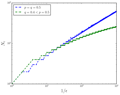
Figure 4: Feature-set scaling of SNS mixed states: Number $N_{\epsilon}$ of nonempty $\epsilon$-cubes as a function of $1/\epsilon$ on a log-log plot. When $p=q$, the scaling relation appears to be power law: $N_{\epsilon}\approx(1/\epsilon)^{1/2}$. When $p\neq q$, $N_{\epsilon}$ scales more slowly than a power law with $1/\epsilon$, seemingly at a rate $N_{\epsilon}\sim\left(\log\frac{1}{\epsilon}\right)^{2}$.

References

- [1] S. Still. EuroPhys. Lett., 85:28005, 2009.
- [2] M. L. Littman, R. S. Sutton, and S. P. Singh. In NIPS, volume 14, pages 1555–1561, 2001.
- [3] N. Tishby and D. Polani. In Perception-action cycle, pages 601–636. Springer, 2011.
- [4] D. Little and F. Sommer. Learning and exploration in action-perception loops. Frontiers in Neural Circuits, 7:37, 2013.
- [5] S. Still and D. Precup. Theory in Biosciences, 131(3):139–148, 2012.
- [6] N. Brodu. Adv. Complex Sys., 14(05):761–794, 2011.
- [7] J. P. Crutchfield. Physica D, 75:11–54, 1994.
- [8] S. Still and J. P. Crutchfield. arXiv:0708.0654.
- [9] T. Berger. Rate Distortion Theory. Prentice-Hall, New York, 1971.
- [10] J. P. Crutchfield and K. Young. Phys. Rev. Let., 63:105–108, 1989.
- [11] C. R. Shalizi and J. P. Crutchfield. J. Stat. Phys., 104:817–879, 2001.
- [12] F. Creutzig, A. Globerson, and N. Tishby. Phys. Rev. E, 79(4):041925, 2009.
- [13] S. Still, J. P. Crutchfield, and C. J. Ellison. CHAOS, 20(3):037111, 2010.
- [14] S. Marzen and J. P. Crutchfield. J. Stat. Phys., 163(6):1312–1338, 2014.
- [15] D. Blackwell. Transactions of the first Prague conference on information theory, Statistical decision functions, Random processes, 28:13–20, 1957. Held at Liblice near Prague from November 28 to 30, 1956.
- [16] L. R. Rabiner and B. H. Juang. IEEE ASSP Magazine, January, 1986.
- [17] E. J. Gilbert. Ann. Math. Stat., pages 688–697, 1959.
- [18] H. Ito, S.-I. Amari, and K. Kobayashi. IEEE Info. Th., 38:324, 1992.
- [19] V. Balasubramanian. Neural Computation, 9:349–368, 1997.
- [20] D. R. Upper. Theory and Algorithms for Hidden Markov Models and Generalized Hidden Markov Models. PhD thesis, University of California, Berkeley, 1997. Published by University Microfilms Intl, Ann Arbor, Michigan.
- [21] This is not necessarily the same as the generative model with minimal generative complexity [48], since a nonunifilar generator with a large number of sparsely-used states might have smaller state entropy than a nonunifilar generator with a small number of equally-used states. And, typically, per our main result, the minimal generative model is usually not the same as the minimal prescient (unifilar) model.
- [22] Cf. Ref. [23]’s discussion of terminology and Ref. [46].
- [23] J. P. Crutchfield and D. P. Feldman. CHAOS, 13(1):25–54, 2003.
- [24] Finite HMMs generate finitary processes, as is bounded from above by the logarithm of the number of HMM states [48].
- [25] T. M. Cover and J. A. Thomas. Elements of Information Theory. Wiley-Interscience, New York, second edition, 2006.
- [26] N. Travers and J. P. Crutchfield. Equivalence of history and generator -machines. arxiv.org:1111.4500.
- [27] One can construct a better feature set simply by applying the causal-state equivalence relation to these length- pasts. We avoid this here since the size of this feature set is more difficult to analyze generically and since the causal-state equivalence relation applied to length- pasts often induces no coarse-graining.
- [28] P. M. Ara, R. G. James, and J. P. Crutchfield. Phys. Rev. E, 93(2):022143, 2016.
- [29] N. F. Travers. Stochastic Proc. Appln., 124(12):4149–4170, 2014.
- [30] C. J. Ellison, J. R. Mahoney, and J. P. Crutchfield. J. Stat. Phys., 136(6):1005–1034, 2009.
- [31] Ya. B. Pesin. University of Chicago Press, 1997.
- [32] We assume here that the lower box-counting dimension and upper box-counting dimension are equivalent.
- [33] S. Still and W. Bialek. Neural Comp., 16(12):2483–2506, 2004.
- [34] C. C. Strelioff and J. P. Crutchfield. Phys. Rev. E, 89:042119, 2014.
- [35] B. D. Johnson, J. P. Crutchfield, C. J. Ellison, and C. S. McTague. arxiv.org:1011.0036.
- [36] S. Marzen and J. P. Crutchfield. Entropy, 17(7):4891–4917, 2015.
- [37] S. Marzen and J. P. Crutchfield. Phys. Lett. A, 380(17):1517–1525, 2016.
- [38] S. Marzen, M. R. DeWeese, and J. P. Crutchfield. Front. Comput. Neurosci., 9:109, 2015.
- [39] S. Marzen and J. P. Crutchfield. arXiv:1611.01099.
- [40] E Ordentlich and T Weissman. Entropy of Hidden Markov Processes and Connections to Dynamical Systems, London Math. Soc. Lecture Notes, 385:117–171, 2011.
- [41] J. Rissanen. IEEE Trans. Info. Th., IT-30:629, 1984.
- [42] A. M. Walker. J. Roy. Stat. Soc. Series B, pages 80–88, 1969.
- [43] C. C. Heyde and I. M. Johnstone. J. Roy. Stat. Soc. Series B, pages 184–189, 1979.
- [44] T.J. Sweeting. Bayesian Statistics, 4:825–835, 1992.
- [45] J. P. Crutchfield and S. Marzen. Phys. Rev. E, 91(5):050106, 2015.
- [46] W. Bialek, I. Nemenman, and N. Tishby. Neural Comp., 13:2409–2463, 2001.
- [47] N. Merhav and M. Feder. IEEE Trans. Info. Th., 44(6):2124–2147, 1998.
- [48] W. Löhr. Models of discrete-time stochastic processes and associated complexity measures. PhD thesis, University of Leipzig, May 2009.
- [49] S.-W. Ho and R. W. Yeung. The interplay between entropy and variational distance. IEEE Trans. Info. Th., 56(12):5906–5929, 2010.
- [50] T. Tao. An Introduction to Measure Theory, volume 126. American Mathematical Society, 2011.
- [51] This upper bound on was noted in Ref. [48].
Supplementary Materials
for