A Universal Ordinary Differential Equation

Abstract.

An astonishing fact was established by Lee A. Rubel (1981): there exists a fixed non-trivial fourth-order polynomial differential algebraic equation (DAE) such that for any positive continuous function $\varphi(t)$ on the reals, and for any positive continuous function $\epsilon(t)$, it has a $\mathcal{C}^{\infty}$ solution with $|y(t)-\varphi(t)|<\epsilon(t)$ for all $t$. Lee A. Rubel provided an explicit example of such a polynomial DAE. Other examples of universal DAE have later been proposed by other authors. However, Rubel’s DAE never has a unique solution, even with a finite number of conditions of the form $y^{(k_{i})}(a_{i})=b_{i}$.

The question whether one can require the solution that approximates $\varphi(t)$ to be the unique solution for a given initial data is a well known open problem [Rubel 1981, page 2], [Boshernitzan 1986, Conjecture 6.2]. In this article, we solve it and show that Rubel’s statement holds for polynomial ordinary differential equations (ODEs), and since polynomial ODEs have a unique solution given an initial data, this positively answers Rubel’s open problem. More precisely, we show that there exists a fixed polynomial ODE such that for any $\varphi(t)$ and $\epsilon(t)$ there exists some initial condition that yields a solution that is $\epsilon(t)$-close to $\varphi(t)$ at all times. In particular, the solution to the ODE is necessarily analytic, and we show that the initial condition is computable from the target function and error function.

1. Introduction

An astonishing result was established by Lee A. Rubel in 1981 [Rub81]. There exists a universal fourth-order algebraic differential equation in the following sense.

[[Rub81]] There exists a non-trivial fourth-order implicit differential algebraic equation

$$P(y^{\prime},y{{}^{\prime\prime}},y{{}^{\prime\prime\prime}},y{{}^{\prime\prime\prime\prime}})=0$$ (1)

where $P$ is a polynomial in four variables with integer coefficients, such that for any continuous function $\varphi$ on $(-\infty,\infty)$ and for any positive continuous function $\epsilon(t)$ on $(-\infty,\infty)$, there exists a $\mathcal{C}^{\infty}$ solution $y$ to (1) such that

$$|y(t)-\varphi(t)|<\epsilon(t)$$

for all $t\in(-\infty,\infty)$.

Even more surprising is the fact that Rubel provided an explicit example of such a polynomial $P$ that is particularly simple:

$$\begin{array}[]{lll}3{y^{\prime}}^{4}y^{{{}^{\prime\prime}}}{y{{}^{\prime\prime\prime\prime}}}^{2}&-4{y^{\prime}}^{4}{y{{}^{\prime\prime\prime}}}^{2}y^{{{}^{\prime\prime\prime\prime}}}+6{y^{\prime}}^{3}{y{{}^{\prime\prime}}}^{2}y{{}^{\prime\prime\prime}}y{{}^{\prime\prime\prime\prime}}+24{y^{\prime}}^{2}{y{{}^{\prime\prime}}}^{4}y{{}^{\prime\prime\prime\prime}}&\\ &-12{y^{\prime}}^{3}y{{}^{\prime\prime}}{y{{}^{\prime\prime\prime}}}^{3}-29{y^{\prime}}^{2}{y{{}^{\prime\prime}}}^{3}{y{{}^{\prime\prime\prime}}}^{2}+12{y{{}^{\prime\prime}}}^{7}&=0.\end{array}$$ (2)

While this result looks very surprising at first sight, Rubel’s proofs turns out to use basic arguments, and can be explained as follows. It uses the following classical trick to build $\mathcal{C}^{\infty}$ piecewise functions: let

$$g(t)=\left\{\begin{array}[]{ll}e^{-1/(1-t^{2})}&\mbox{ for }-1<t<1\\ 0&\mbox{ otherwise.}\end{array}\right.$$

It is not hard to see that function $g$ is $C^{\infty}$ and Figure 1 shows that $g$ looks like a “bump”. Since it satisfies

$$\tfrac{g^{\prime}(t)}{g(t)}=-\frac{2t}{(1-t^{2})^{2}},$$

then

$$g^{\prime}(t)(1-t^{2})^{2}+g(t)2t=0$$

and $f(t)=\int_{0}^{t}g(u)du$ satisfies the polynomial differential algebraic equation

$$f^{\prime\prime}(1-t^{2})^{2}+f^{\prime}(t)2t=0.$$

Since this equation is homogeneous, it also holds for $af+b$ for any $a$ and $b$. The idea is then to obtain a fourth order DAE that is satisfied by every function $y(t)=\gamma f(\alpha t+\beta)+\delta$, for all $\alpha,\beta,\gamma,\delta$. After some computations, Rubel obtained the universal differential equation (2).

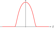
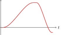
Figure 1. On left, graphical representation of function $g$. On right, two $S$-modules glued together.

Functions of the type $y(t)=\gamma f(\alpha t+\beta)+\delta$ generate what Rubel calls $S$-modules: a function that values $A$ at $a$, $B$ at $b$, is constant on $[a,a+\delta]$, monotone on $[a+\delta,b-\delta]$, constant on $[b-\delta,b]$, by an appropriate choice of $\alpha,\beta,\gamma,\delta$. Summing $S$-modules corresponds to gluing then together, as is depicted in Figure 1. Note that finite, as well as infinite sums of $S$-modules still satisfy the equation (2) and thus any piecewise affine function (and hence any continuous function) can be approximated by an appropriate sum of $S$-modules. This concludes Rubel’s proof of universality.

As one can see, the proof turns out to be frustrating because the equation essentially allows any behavior. This may be interpreted as merely stating that differential algebraic equations is simply too lose a model. Clearly, a key point is that this differential equation does not have a unique solution for any given initial condition: this is the core principle used to glue a finite or infinite number of $S$-modules and to approximate any continuous function. Rubel was aware of this issue and left open the following question in [Rub81, page 2].

“It is open whether we can require in our theorem that the solution that approximates $\varphi$ to be the unique solution for its initial data.”

Similarly, the following is conjectured in [Bos86, Conjecture 6.2].

“Conjecture. There exists a non-trivial differential algebraic equation such that any real continuous function on $\mathbb{R}$ can be uniformly approximated on all of $\mathbb{R}$ by its real-analytic solutions”

The purpose of this paper is to provide a positive answer to both questions. We prove that a fixed polynomial ordinary differential equations (ODE) is universal in above Rubel’s sense. At a high level, our proofs are based on ordinary differential equation programming. This programming is inspired by constructions from our previous paper [BGP16a]. Here, we mostly use this programming technology to achieve a very different goal and to provide positive answers to these above open problems.

We also believe they open some lights on computability theory for continuous-time models of computations. In particular, it follows that concepts similar to Kolmogorov complexity can probably be expressed naturally by measuring the complexity of the initial data of a (universal-) polynomial ordinary differential equation for a given function. We leave this direction for future work.

The current article is an extended version of [BP17]: here all proofs are provided, and we extend the statements by proving that the initial condition can always be computed from the function in the sense of Computable Analysis.

1.1. Related work and discussions

First, let us mention that Rubel’s universal differential equation has been extended in several papers. In particular, Duffin proved in [Duf81] that implicit universal differential equations with simpler expressions exists, such as

$$n^{2}y^{{}^{\prime\prime\prime\prime}}{y^{\prime}}^{2}+3n(1-n)y^{{}^{\prime\prime\prime}}y^{{}^{\prime\prime}}y^{\prime}+(2n^{2}-3n+1){y^{{}^{\prime\prime}}}^{3}=0$$

for any $n>3.$ The idea of [Duf81] is basically to replace the $\mathcal{C}^{\infty}$ function $g$ of [Rub81] by some piecewise polynomial of fixed degree, that is to say by splines. Duffin also proves that considering trigonometric polynomials for function $g(x)$ leads to the universal differential equation

$$ny^{{}^{\prime\prime\prime\prime}}{y^{\prime}}^{2}+(2-3n)y^{{}^{\prime\prime\prime}}y^{{}^{\prime\prime}}y^{\prime}+2(n-1){y^{\prime\prime}}^{3}=0.$$

This is done at the price of approximating function $\varphi$ respectively by splines or trigonometric splines solutions which are $\mathcal{C}^{n}$ (and $n$ can be taken arbitrary big) but not $\mathcal{C}^{\infty}$ as in [Rub81]. Article [Bri02] proposes another universal differential equation whose construction is based on Jacobian elliptic functions. Notice that [Bri02] is also correcting some statements of [Duf81].

All the results mentioned so far are concerned with approximations of continuous functions over the whole real line. Approximating functions over a compact domain seems to be a different (and somewhat easier for our concerns) problem, since basically by compactness, one just needs to approximate the function locally on a finite number of intervals. A 1986 reference survey discussing both approximation over the real line and over compacts is [Bos86]. Recently, over compact domains, the existence of universal ordinary differential equation $\mathcal{C}^{\infty}$ of order $3$ has been established in [CJ16]: it is shown that for any $a<b$, there exists a third order $\mathcal{C}^{\infty}$ differential equation $y^{\prime\prime\prime}=F(y,y^{\prime},y^{\prime\prime})$ whose solutions are dense in $\mathcal{C}^{0}([a,b])$. Notice that this is not obtained by explicitly stating such an order $3$ universal ordinary differential, and that this is a weaker notion of universality as solutions are only assumed to be arbitrary close over a compact domain and not all the real line. Order $3$ is argued to be a lower bound for Lipschitz universal ODEs [CJ16].

Rubel’s result has sometimes been considered to be the equivalent, for analog computers, of the universal Turing machines. This includes Rubel’s paper motivation given in [Rub81, page 1]. We now discuss and challenge this statement.

Indeed, differential algebraic equations are known to be related to the General Purpose Analog Computer (GPAC) of Claude Shannon [Sha41], proposed as a model of the Differential Analysers [Bus31], a mechanical programmable machine, on which he worked as an operator. Notice that the original relations stated by Shannon in [Sha41] between differential algebraic equations and GPACs have some flaws, that have been corrected later by [PE74] and [GC03]. Using the better defined model of GPAC of [GC03], it can be shown that functions generated by GPAC exactly correspond to polynomial ordinary differential equations. Some recent results have established that this model, and hence polynomial ordinary differential equations can be related to classical computability [BCGH07] and complexity theory [BGP16a].

However, we do not really agree with the statement that Rubel’s result is the equivalent, for analog computers, of the universal Turing machines. In particular, Rubel’s notion of universality is completely different from those in computability theory. For a given initial data, a (deterministic) Turing machine has only one possible evolution. On the other hand, Rubel’s equation does not dictate any evolution but rather some conditions that any evolution has to satisfy. In other words, Rubel’s equation can be interpreted as the equivalent of an invariant of the dynamics of (Turing) machines, rather than a universal machine in the sense of classical computability.

Notice that while several results have established that (polynomial) ODEs are able to simulate the evolution of Turing machines (see e.g. [BCGH07, GCB08, BGP16a]), the existence of a universal ordinary differential equation does not follow from them. To understand the difference, let us restate the main result of [GCB08], of which [BGP16a] is a more advanced version for polynomial-time computable functions.

Theorem 1.

A function $f:[a,b]\to\mathbb{R}$ is computable (in the framework of Computable Analysis) if and only if there exists some polynomials $p:\mathbb{R}^{n}\to\mathbb{R}^{n}$, $p_{0}:\mathbb{R}\to\mathbb{R}$ with computable coefficients and $\alpha_{1},\ldots,\alpha_{n-1}$ computable reals such that for all $x\in[a,b]$, the solution $y:\mathbb{R}_{\geqslant 0}\to\mathbb{R}^{n}$ to the Cauchy problem

$$y(0)=(\alpha_{1},\ldots,\alpha_{n-1},p_{0}(x)),\qquad y^{\prime}=p(y)$$

satisfies that for all $t\geqslant 0$ that

$$|f(x)-y_{1}(t)|\leqslant y_{2}(t)\quad\text{and}\quad\lim_{t\rightarrow\infty}y_{2}(t)=0.$$

Since there exists a universal Turing machine, there exists a “universal” polynomial ODE for computable functions. But there are major differences between Theorem 1 and the result of this paper (Theorem 2). Even if we have a strong link between the Turing machines’s configuration and the evolution of the differential equation, this is not enough to guarantee what the trajectory of the system will be at all times. Indeed, Theorem 1 only guarantees that $y_{1}(t)\rightarrow f(x)$ asymptotically. On the other hand, Theorem 2 guarantees the value of $y_{1}(t)$ at all times. Notice that our universality result also applies to functions that are not computable (in which case the initial condition is computable from the function but still not computable).

We would like to mention some implications for experimental sciences that are related to the classical use of ODEs in such contexts. Of course, we know that this part is less formal from a mathematical point of view, but we believe this discussion has some importance: A key property in experimental sciences, in particular physics is analyticity. Recall that a function is analytic if it is equal to its Taylor expansion in any point. It has sometimes been observed that “natural” functions coming from Nature are analytic, even if this cannot be a formal statement, but more an observation (see e.g. [BC08, Moo90, KM99]). We obtain a fixed universal polynomial ODE, so in particular all its solution must be analytic, and it follows that universality holds even with analytic functions. All previous constructions mostly worked by gluing together $\mathcal{C}^{\infty}$ or $\mathcal{C}^{n}$ functions, and as it is well known “gluing” of analytic functions is impossible. We believe this is an important difference with previous works.

As we said, Rubel’s proof can be seen as an indication that (fourth-order) polynomial implicit DAE is too loose model compared to classical ODEs, allowing in particular to glue solutions together to get new solutions. As observed in many articles citing Rubel’s paper, this class appears so general that from an experimental point of view, it makes littles sense to try to fit a differential model because a single equation can model everything with arbitrary precision. Our result implies the same for polynomial ODEs since, for the same reason, a single equation of sufficient dimension can model everything.

Notice that our constructions have at the end some similarities with Voronin’s theorem. This theorem states that Riemann’s $\zeta$ function is such that for any analytic function $f(z)$ that is non-vanishing on a domain $U$ homeomorphic to a closed disk, and any $\epsilon>0$, one can find some real value $t$ such that for all $z\in U$, $|\zeta(z+it)-f(z)|<\epsilon$. Notice that $\zeta$ function is a well-known function known not to be solution of any polynomial DAE (and consequently polynomial ODE), and hence there is no clear connection to our constructions based on ODEs. We invite to read the post [LR] in “Gödel’s Lost Letter and P=NP” blog for discussions about potential implications of this surprising result to computability theory.

1.2. Formal statements

Our results are the following:

Theorem 2 (Universal PIVP).

There exists a fixed polynomial vector $p$ in $d$ variables with rational coefficients such that for any functions $f\in C^{0}(\mathbb{R})$ and $\varepsilon\in C^{0}(\mathbb{R},\mathbb{R}_{>0})$, there exists $\alpha\in\mathbb{R}^{d}$ such that there exists a unique solution $y:\mathbb{R}\rightarrow\mathbb{R}^{d}$ to $y(0)=\alpha$, $y^{\prime}=p(y).$ Furthermore, this solution satisfies that $|y_{1}(t)-f(t)|\leqslant\varepsilon(t)$ for all $t\in\mathbb{R}$, and it is analytic.

Furthermore, $\alpha$ can be computed from $f$ and $\varepsilon$ in the sense of Computable Analysis, more precisely $(f,\varepsilon)\mapsto\alpha$ is $([\rho\to\rho]^{2},\rho^{d})$-computable (refer to Section 2.3 for formal definitions).

It is well-known that polynomial ODEs can be transformed into DAEs that have the same analytic solutions, see [CPSW05] for example. The following then follows for DAEs.

Theorem 3 (Universal DAE).

There exists a fixed polynomial $p$ in $d+1$ variables with rational coefficients such that for any functions $f\in C^{0}(\mathbb{R})$ and $\varepsilon\in C^{0}(\mathbb{R},\mathbb{R}_{>0})$, there exists $\alpha_{0},\ldots,\alpha_{d-1}\in\mathbb{R}$ such that there exists a unique analytic solution $y:\mathbb{R}\rightarrow\mathbb{R}$ to $y(0)=\alpha_{0},y^{\prime}(0)=\alpha_{1},\ldots,y^{(d-1)}(0)=\alpha_{d-1}$, $p(y,y^{\prime},\ldots,y^{d})=0.$ Furthermore, this solution satisfies that $|y(t)-f(t)|\leqslant\varepsilon(t)$ for all $t\in\mathbb{R}$.

Furthermore, $\alpha$ can be computed from $f$ and $\varepsilon$ in the sense of Computable Analysis, more precisely $(f,\varepsilon)\mapsto\alpha$ is $([\rho\to\rho]^{2},\rho^{d})$-computable (refer to Section 2.3 for formal definitions).

Remark 4.

Notice that both theorems apply even when $f$ is not computable. In this case, the initial condition(s) $\alpha$ exist but are not computable. We will prove that $\alpha$ is always computable from $f$ and $\varepsilon$, that is the mapping $(f,\varepsilon)\mapsto\alpha$ is computable in the framework of Computable Analysis, with an adequate representation of $f,\varepsilon$ and $\alpha$.

Remark 5.

Notice that we do not provide explicitly in this paper the considered polynomial ODE, nor its dimension $d$. But it can be derived by following the constructions. We currently estimate $d$ to be more than three hundred following the precise constructions of this paper (but also to be very far from the optimal). We did not try to minimize $d$ in the current paper, as we think our results are sufficiently hard to be followed in this paper for not being complicated by considerations about optimization of dimensions.

Remark 6.

Both theorems are stated for total functions $f$ and $\varepsilon$ over $\mathbb{R}$. It trivially applies to any continuous partial function that can be extended to a continuous function over $\mathbb{R}$. In particular, it applies to any functions over $[a,b]$. It is not hard to see that it also applies to functions over $(a,b)$ by rescaling $\mathbb{R}$ into $(a,b)$ using the cotangent:

$$z(t)=y\left(-\cot\left(\tfrac{t-a}{b-a}\pi\right)\right)\quad\text{satisfies}\quad z^{\prime}(t)=\phi^{\prime}(t)p(z(t)),\quad\phi^{\prime}(t)=\tfrac{\pi}{b-a}(1+\phi(t)^{2}).$$

More complex domains such as $[a,b)$ and $(a,b]$ (with $a$ possibly infinite) can also be obtained using a similar method.

Remark 7.

Since the solution of a polynomial (or analytic) differential equation is analytic, our results can be compared with the problem of building uniform approximations of continuous function on the real line by analytic ones, and hence can be seen as a strengthening of such results (see e.g. [Kap55]).

Remark 8.

Let $Y(\alpha)$ be the solution given by Theorem 2 satisfying $Y(\alpha)(0)=\alpha$. Note that the theorem does not specify the existence of $Y(\alpha)(t)$ for all $t$ and $\alpha$. In fact, because of function $\mathtt{fastgen}$ in what follows, $Y(\alpha)$ will explode in finite time for all $\alpha$ that have certain coordinates rational, and the length of the interval of life depends on $\alpha$. Therefore, given $\alpha\in\mathbb{R}^{d}$, any ball around $\alpha$ contains a $\beta$ such that $Y(\beta)$ explodes in finite time for the function $Y$ corresponding to our constructions.

Remark 9.

It may look at first like that Theorem 2 violates Brouwer’s Invariance of domain but this is not the case. Indeed, continuing with the notation of above remark, $Y$ is continuous and $Y$ is injective with image in $S:=\bigcup_{a<b}C^{0}((a,b),\mathbb{R}^{d})$ (see Remark 8 about domains). Clearly $S$ is of much higher dimension than $\alpha\in\mathbb{R}^{d}$ but $Y$ is not dense in $S$ so there is no contradiction. On the other hand, if we only consider the first coordinate $Y_{1}$, then $Y_{1}$ is dense in $C^{0}(\mathbb{R},\mathbb{R})$ but is not injective.

1.3. Overview of the proof

A first a priori difficulty is that if one considers a fixed polynomial ODE $y^{\prime}=p(y)$, one could think that the growth of its solutions is constrained by $p$ and thus cannot be arbitrary. This would then prevent us from building a universal ODE simply because it could not grow fast enough. This fact is related to Emil Borel’s conjecture in [Bor99] (see also [Har12]) that a solution, defined over $\mathbb{R}$, to a system with $n$ variables has growth bounded by roughly $e_{n}(x)$, the $n-$th iterate of $\exp$. The conjecture is proved for $n=1$ [Bor99], but has been proven to be false for $n=2$ in [Vij32] and [BBV37]. Bank [Ban75] then adapted the previous counter-examples to provide a DAE whose non-unique increasing real-analytic solutions at infinity do not have any majorant. See the discussions (and Conjecture 6.1) in [Bos86] for discussions about the growth of solutions of DAEs, and their relations to functions $e_{n}(x)$.

Thus, the first important part of this paper is to refine Bank’s counter-example to build fastgen, a fast-growing function that satisfies even stronger properties. The second major ingredient is to be able to approximate a function with arbitrary precision everywhere. Since this is a difficult task, we use fastgen to our advantage to show that it is enough to approximate functions that are bounded and change slowly (think 1-Lipschitz, although the exact condition is more involved). That is to say, to deal with the case where there is no problem about the growth and rate of change of functions in some way. This is the purpose of the function pwcgen which can build arbitrary almost piecewise constant functions as long as they are bounded and change slowly.

It should be noted that in the entire paper, we construct generable functions (in several variables) (see Section 2.1). For most of the constructions, we only use basic facts like the fact that generable functions are stable under arithmetic, composition and ODE solving. We know that generable functions satisfy polynomial partial equations and use this fact only at the very end to show that the generable approximation that we have built, in fact, translates to a polynomial ordinary differential equation.

The rest of the paper is organised as follows. In Section 2, we recall some concepts and results from other articles. The main purpose of this section is to present Theorem 20. This theorem is the analog equivalent of doing an assignment in a periodic manner. Section 3 is devoted to fastgen, the fast-growing function. In Section 4, we show how to generate a sequence of dyadic rationals. In Section 5, we show how to generate a sequence of bits. In Section 6, we show how to leverage the two previous sections to generate arbitrary almost piecewise constant functions. Section 7 is then devoted to the proof of our main theorem.

2. Concepts and results from previous work

2.1. Generable functions

The following concept can be attributed to [Sha41]: a function $f:\mathbb{R}\to\mathbb{R}$ is said to be a PIVP (Polynomial Initial Value Problem) function if there exists a system of the form $y^{\prime}=p(y)$, where $p$ is a (vector of) polynomial, with $f(t)=y_{1}(t)$ for all $t$, where $y_{1}$ denotes first component of the vector $y$ defined in $\mathbb{R}^{d}$. We need in our proof to extend this concept to talk about multivariate functions. In [BGP17], we introduced the following class, which can be seen as extensions of [GBC09]. Let $\mathbb{K}$ be the smallest generable field (see [BGP17] for formal definitions and properties), the reader only needs to know that $\mathbb{Q}\subseteq\mathbb{K}\subseteq\mathbb{R}_{P}$ where $\mathbb{R}_{P}$ is the set of polynomial-time computable reals, and $\mathbb{K}$ is closed under images of generable functions.

[Generable function] Let $d,e\in\mathbb{N}$, $I$ be an open and connected subset of $\mathbb{R}^{d}$ and $f:I\rightarrow\mathbb{R}^{e}$. We say that $f$ is generable if and only if there exists an integer $n\geqslant e$, a $n\times d$ matrix $p$ consisting of polynomials with coefficients in $\mathbb{K}$, $x_{0}\in\mathbb{K}^{d}$, $y_{0}\in\mathbb{K}^{n}$ and $y:I\rightarrow\mathbb{R}^{n}$ satisfying for all $x\in I$:

• $y(x_{0})=y_{0}$ and $J_{y}(x)=p(y(x))$ $\blacktriangleright$ $y$ satisfies a polynomial differential equation,

• $f(x)=(y_{1}(x),\ldots,y_{e}(x))$ $\blacktriangleright$ the components of $f$ are components of $y$.

This class strictly generalizes functions generated by polynomial ODEs. Indeed, in the special case of $d=1$ (the domain of the function has dimension $1$), the above definition is equivalent to saying that $y^{\prime}=p(y)$ for some polynomial $p$. The interested reader can read more about this in [BGP17].

For the purpose of this paper, we will need to consider a slight generalisation of this notion where the initial condition is considered to be (depending of) a parameter, therefore defining not just a single function but a family of function, and most importantly, all sharing the same differential equation. Formally:

[Uniformly-generable function] Let $d,m,e\in\mathbb{N}$, $I$ be an open and connected subset of $\mathbb{R}^{d}$, $\Gamma\subseteq\mathbb{R}^{m}$, and $f:\Gamma\times I\rightarrow\mathbb{R}^{e}$. We say that $f$ is uniformly-generable if and only if there exists an integer $n\geqslant e$, a $n\times d$ matrix $p$ consisting of polynomials with coefficients in $\mathbb{K}$, $x_{0}\in\mathbb{K}^{d}\cap I$ and a $(\rho^{m},\rho^{n})-$computable function $y_{0}:\Gamma\to\mathbb{R}^{n}$ such that for all $\gamma\in\Gamma$, there exists $y:I\rightarrow\mathbb{R}^{n}$ satisfying for all $x\in I$:

• $y(x_{0})=y_{0}(\gamma)$ and $J_{y}(x)=p(y(x))$ $\blacktriangleright$ $y$ satisfies a polynomial differential equation

• $f(\gamma;x)=(y_{1}(x),\ldots,y_{e}(x))$ $\blacktriangleright$ the components of $f$ are components of $y$.

For readability, we will distinguish parameters from variables using a semicolon, for example $f(\gamma;x)$ is parameterized by $\gamma$. This should make it clear from the context what is considered as parameter and what is considered as a variable.

Remark 10.

Although we have chosen $x_{0}$ and the coefficients of $p$ to be in $\mathbb{K}$ in the definition above, it is clear that we can change this set at the cost of increasing the set $\Gamma$ of parameters. For example we could take all coefficients to be rational or in $\left\{0,1\right\}$ by adding one extra parameter per coefficient and hence “hiding” them in $y_{0}$. The only real constraint is that since $y_{0}$ must remain computable, we still need all elements of $\mathbb{K}$ to be computable.

For the purpose of this paper, the reader only needs to know that the class of generable functions enjoys many stability properties that make it easy to create new functions from basic operations. Informally, one can add, subtract, multiply, divide and compose them at will, the only requirement is that the domain of definition must always be connected. In particular, the class of generable functions contains some common mathematical functions:

• (multivariate) polynomials;

• trigonometric functions: $\sin$, $\cos$, $\tan$, etc;

• exponential and logarithm: $\exp$, $\ln$;

• hyperbolic trigonometric functions: $\sinh$, $\cosh$, $\tanh$.

Two famous examples of functions that are not in this class are the $\zeta$ and $\Gamma$, we refer the reader to [BGP17] and [GBC09] for more information.

A nontrivial fact is that generable functions are always analytic. This property is well-known in the one-dimensional case but is less obvious in higher dimensions, see [BGP17] for more details. Moreover, generable functions satisfy the following crucial properties.

Lemma 11 (Closure properties of generable functions [BGP17]).

Let $f:\subseteq\mathbb{R}^{d}\rightarrow\mathbb{R}^{n}$ and $g:\subseteq\mathbb{R}^{e}\rightarrow\mathbb{R}^{m}$ be generable functions. Then $f+g$, $f-g$, $fg$, $\tfrac{f}{g}$ and $f\circ g$ are generable.

Lemma 12 (Generable functions are closed under ODE [BGP17]).

Let $d\in\mathbb{N}$, $J\subseteq\mathbb{R}$ an interval, $f:\subseteq\mathbb{R}^{d}\rightarrow\mathbb{R}^{d}$ generable, $t_{0}\in J\cap\mathbb{K}$ and $y_{0}\in\operatorname{dom}{f}\cap\mathbb{K}^{d}$. Assume there exists $y:J\rightarrow\operatorname{dom}{f}$ satisfying

$$y(t_{0})=y_{0},\qquad y^{\prime}(t)=f(y(t))$$

for all $t\in J$, then $y$ is generable (and unique).

Those results can be generalised to uniformly-generable functions with the obvious restrictions on the domains and the roles of parameters. For example, if $f(\alpha;x)$ and $g(\beta;y)$ are uniformly-generable over $A\times X$ and $B\times Y$ respectively, then $h(\alpha,\beta;y):=f(\alpha;g(\beta;y))$ is uniformly-generable over $A\times B\times Y$. We will use those facts implicitly, and in particular the following result:

Theorem 13 (Uniformly-generable functions are closed under ODE).

Let $d,m\in\mathbb{N}$, $\Gamma\subseteq\mathbb{R}^{m}$, $t_{0}\in\mathbb{K}$, $J$ an open interval containing $t_{0}$, $f_{0}:\Gamma\to\mathbb{R}^{d}$ a $(\rho^{m},\rho^{d})-$computable function and $F:\subseteq\Gamma\times\mathbb{R}^{d}\rightarrow\mathbb{R}^{d}$ uniformly-generable. Assume that there exists $f:\Gamma\times J\rightarrow\mathbb{R}^{d}$ satisfying

$$f(\gamma;t_{0})=f_{0}(\gamma),\qquad\tfrac{\partial f}{\partial t}(\gamma;t)=F(\gamma;f(\gamma;t))$$

for all $\gamma\in\Gamma$ and $t\in J$. Then $f$ is uniformly-generable (and unique).

Proof 2.1.

Apply Definition 2.1 to $F$ to get $n\in\mathbb{N}$, $x_{0}\in\mathbb{K}^{n}$, $y_{0}:\Gamma\to\mathbb{R}^{n}$ computable and $p$ polynomial matrix with coefficients in $\mathbb{K}$. Then given $\gamma\in\Gamma$, there exists $y:\subseteq\mathbb{R}^{d}\to\mathbb{R}^{n}$ such that

$$y(x_{0})=y_{0}(\gamma),\qquad J_{y}(x)=p(y(x))$$

and $F(\gamma;x)=(y_{1}(x),\ldots,y_{d}(x))=:y_{1..d}(x)$ for all $(\gamma,x)\in\operatorname{dom}{F}$. Let $z(t)=y(f(\gamma;t))$ which is well-defined by assumption and check that

$$z^{\prime}(t)=J_{y}(f(\gamma;t))\tfrac{\partial f}{\partial t}(\gamma;t)=p(y(f(\gamma;t)))F(\gamma;f(\gamma;t))=p(z(t))z_{1..d}(t)=q(z(t))$$

for some polynomial $q$ that does not depend on $\gamma$, and $z(t_{0})=y(f(\gamma;t_{0}))=y(f_{0}(\gamma))$ which is a computable function of $\gamma$ since $f_{0}$ is computable and $(\gamma,x)\mapsto y(x)$ is also computable (note that $y$ depends on $\gamma$) by Proposition 14.

An important point, which we have in fact already used in the proof of the previous proposition, is that generable functions are always computable, in the sense of Computable Analysis.

Proposition 14 (Generable implies computable).

Assume $f:\Gamma\times I\rightarrow\mathbb{R}^{e}$ is uniformly generable according to Definition 2.1: Hence there is a $(\rho^{m},\rho^{n})-$computable function $y_{0}:\Gamma\to\mathbb{R}^{n}$ and a $n\times d$ matrix $p$ consisting of polynomials with coefficients in $\mathbb{K}$, $x_{0}\in\mathbb{K}^{d}$ that define $y(\gamma;x_{0})=y_{0}(\gamma)$ and $J_{y}(x)=p(y(\gamma;x))$. Then the function that maps $(\gamma,x)\in\Gamma\times I$ to $y(\gamma;x)$ is $([\rho^{m},\rho^{d}],\rho^{n})-$computable.

Proof 2.2.

We established in proposition [BGP17, Proposition 31] that $y(x)$ is necessarily real-analytic on some neighbourhood $V=V(x)$ of $x$ for all $x$ that corresponds to some point of the domain of $f$.

Some explicit upper bound on the radius of convergence is provided by [PG16, Theorem 5]: Assuming $t_{0}=0$, $k=\deg(p)\geq 2$, $\alpha=\max(1,\left\lVert{y_{0}}\right\rVert)$, the radius is at least $1/M$ with $M=M(y_{0})=(k-1)\Sigma p\alpha^{k-1}$, where $\Sigma p$ is basically the sum of the absolute value of the coefficients of polynomials in matrix $p$.

Consequently, using classical techniques for evaluating a converging power series whose convergence radius is known up to a given precision (by restricting the sum up to suitable index) we get that $y$ is computable over the ball $V(y_{0})$ of radius $1/(2M)$.

Computability of $y$ then follows from classical analytic continuation techniques: A Turing machine can then extend the computation starting from a new point $y_{1}$ in $V(y_{0}(\gamma))$, and then repeat the above process to compute $y$ over some ball $V(y_{1})$ of radius $1/(2M(y_{1}))$, and so on. Repeating the process, eventually, it will reach $x$ and will be able to compute $y(x)$. Refer to [KTZ18, Thi18] for similar techniques and a finer complexity analysis.

2.2. Helper functions and constructions

We mentioned earlier that a number of common mathematical functions are generable. However, for our purpose, we will need less common functions that one can consider to be programming gadgets.

Remark 15.

In this subsection, some of the functions will be introduced as mapping arguments to value, i.e. as usual mathematical functions, but some others by the properties of their solutions (e.g. $\mathtt{reach}$, $\mathtt{pereach}$, $\mathtt{pil})$. In the latter case, an explicit expression of a function satisfying those properties can be found in the proof.

One such operation is rounding (computing the nearest integer). Note that, by construction, generable functions are analytic and in particular must be continuous. It is thus clear that we cannot build a perfect rounding function and in particular we have to compromise on two aspects:

• we cannot round numbers arbitrarily close to $n+\tfrac{1}{2}$ for $n\in\mathbb{Z}$ because of continuity: thus the function takes a parameter $\lambda$ to control the size of the “zone” around $n+\tfrac{1}{2}$ where the function does not round properly;

• we cannot round without error due to the uniqueness of analytic functions: thus the function takes a parameters $\mu$ that controls how good the approximation must be.

Lemma 16 (Round, [BGP17]).

There exists a generable function $\mathtt{round}$ such that for any $n\in\mathbb{Z}$, $x\in\mathbb{R}$, $\lambda>2$ and $\mu\geqslant 0$:

• if $x\in\left[n-\frac{1}{2},n+\frac{1}{2}\right]$ then $|\mathtt{round}(x,\mu,\lambda)-n|\leqslant\frac{1}{2}$;

• if $x\in\left[n-\frac{1}{2}+\frac{1}{\lambda},n+\frac{1}{2}-\frac{1}{\lambda}\right]$ then $|\mathtt{round}(x,\mu,\lambda)-n|\leqslant e^{-\mu}$.

Another very useful operation is the analog equivalent of a discrete assignment, done in a periodic manner. More precisely, we consider a particular class of ODEs

$$y^{\prime}(t)=\mathtt{pereach}(t,\phi(t),y(t),g(t))$$

adapted from the constructions of [BGP16a], where $g$ and $\phi$ are sufficiently nice functions. Solutions to this equation alternate between two behaviours, for all $n\in\mathbb{N}$:

• During $J_{n}=[n,n+\tfrac{1}{2}]$, the system performs $y(t)\rightarrow\overline{g}$ for some $\bar{g}$ satisfying $\min_{t\in J_{n}}g(t)\leqslant\overline{g}\leqslant\max_{t\in J_{n}}g(t)$ (note that this is voluntarily underspecified). So in particular, if $g(t)\approx\bar{g}$ over this time interval, then $y(t)\rightarrow\bar{g}$ and the system performs an “assignment” in the sense that $y(n+\tfrac{1}{2}):=\bar{g}$. Then $\phi$ controls how good the convergence is: the error is of the order of $e^{-\phi}$.

• During $J_{n}^{\prime}=[n+\tfrac{1}{2},n+1]$, the systems tries to keep $y$ constant, ie $y^{\prime}\approx 0$. More precisely, the system enforces that $|y^{\prime}(t)|\leqslant e^{-\phi(t)}$.

As a result of this behavior, if $g(t)\approx\bar{g}$ for $t\in[n,n+\tfrac{1}{2}]$ then the system performs the “assignment” $y(n+1):=\bar{g}$ with some error that is exponential small in $\phi$.

We now go to the proof of the existence of such a function $\mathtt{pereach}$ (formally stated as Theorem 20): We will need the following bound on $\tanh$, which essentially tells us that $\tanh(t)$ gets exponentially close (in $|t|$) to $\pm 1$ as $t\to\pm\infty$.

Lemma 17.

For any $t\in\mathbb{R}$, $|\tanh(t)-\mathtt{sgn}(t)|\leqslant e^{-|t|}$.

Lemma 18 (Reach, [BGP16b]).

There exists a generable function $\mathtt{reach}$ such that for any $\phi\in C^{0}(\mathbb{R}_{\geqslant 0})$, $g\in C^{0}(\mathbb{R})$ and $y_{0}\in\mathbb{R}$, the unique solution to

$$y(0)=y_{0},\qquad y^{\prime}(t)=\phi(t)\mathtt{reach}(g(t)-y(t))$$

exists over $\mathbb{R}_{\geqslant 0}$. Furthermore, for any $I=[a,b]\subseteq[0,+\infty)$, if there exists $\bar{g}\in\mathbb{R}$ and $\eta\in\mathbb{R}_{\geqslant 0}$ such that $|g(t)-\bar{g}|\leqslant\eta$ for all $t\in I$, then for all $t\in I$,

$$|y(t)-\bar{g}|\leqslant\eta+\exp\left(-\int_{a}^{t}\phi(u)du\right)\qquad\text{whenever }\int_{a}^{t}\phi(u)du\geqslant 1.$$

Furthermore, for all $t\in I$,

$$\min(\bar{g}-\eta,y(a))\leqslant y(t)\leqslant\max(\bar{g}+\eta,y(a))$$

and in particular

$$|y(t)-\bar{g}|\leqslant\max(\eta,|y(a)-\bar{g}|).$$

Proof 2.3 (Proof Remark).

The statement of [BGP16b, Lemma 40] only contains the first and third inequalities but in fact the proof also contains the second inequality (which is strictly stronger than the third but less immediate to use).

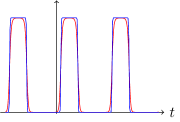
Figure 2. Illustration of $\mathtt{pil}(\mu,\cdot)$ from Lemma 19 for various values of $\mu$: it has period $1$, is very small ($\leqslant e^{-\mu}$) half of the time, and the integral of the remaining half is at least $1$.

Lemma 19 (Periodic integral-low, see Figure 2).

There exists a generable function $\mathtt{pil}:\mathbb{R}_{\geqslant 0}\times\mathbb{R}\rightarrow\mathbb{R}_{\geqslant 0}$ such that:

• $\mathtt{pil}(\mu,\cdot)$ is 1-periodic, for any $\mu\in\mathbb{R}_{\geqslant 0}$;

• $\int_{0}^{1/2}\mathtt{pil}(\mu(t),t)dt\geqslant 1$ for any $\mu\in C^{0}(\mathbb{R}_{\geqslant 0})$;

• $|\mathtt{pil}(\mu,t)|\leqslant e^{-\mu}$ for any $\mu\in\mathbb{R}_{\geqslant 0}$ and $t\in\left[\tfrac{1}{2},1\right]$.

Proof 2.4.

For any $t\in\mathbb{R}$ and $\mu\in\mathbb{R}_{\geqslant 0}$, let

$$\mathtt{pil}(\mu,t)=A\left(1+\tanh\big{(}2(\sin(2\pi t)-\tfrac{1}{2})(A+\mu)\big{)}\right).$$

where $A=3$. Clearly $\mathtt{pil}$ is generable and 1-periodic in $t$. Let $\mu\in\mathbb{R}_{\geqslant 0}$ and $t\in[\tfrac{1}{2},1]$, then

$$\sin(2\pi t) \leqslant 0$$

$$2(\sin(2\pi t)-\tfrac{1}{2})(A+\mu) \leqslant-A-\mu$$

$$|\tanh(2(\sin(2\pi t)-\tfrac{1}{2})(A+\mu))-(-1)| \leqslant e^{-A-\mu}$$ using Lemma 17

$$A|\tanh(2(\sin(2\pi t)-\tfrac{1}{2})(A+\mu))-(-1)| \leqslant Ae^{-A-\mu}$$

$$|\mathtt{pil}(\mu,t)| \leqslant e^{-\mu}.$$

Let $\mu\in C^{0}(\mathbb{R}_{\geqslant 0})$ and $t\in[0,\tfrac{1}{2}]$. Observe that $\mathtt{pil}(\mu(t),t)\geqslant 0$ and, furthermore, if $t\in[\tfrac{1}{8},\tfrac{3}{8}]$ then

$$\sin(2\pi t) \geqslant\frac{\sqrt{2}}{2}$$

$$2(\sin(2\pi t)-\tfrac{1}{2})(A+\mu(t)) \geqslant\sqrt{2}-1 \text{since }A+\mu(t)\geqslant 1$$

$$\tanh(2(\sin(2\pi t)-\tfrac{1}{2})(A+\mu(t))) \geqslant\tanh(\sqrt{2}-1)\geqslant\frac{1}{3}$$

$$\mathtt{pil}(\mu(t),t) \geqslant\tfrac{4}{3}A.$$

It follows that

$$\int_{0}^{\tfrac{1}{2}}\mathtt{pil}(\mu(t),t)dt\geqslant\int_{\tfrac{1}{8}}^{\tfrac{3}{8}}\mathtt{pil}(\mu(t),t)dt\geqslant\left(\frac{3}{8}-\frac{1}{8}\right)\frac{4}{3}A\geqslant\frac{A}{3}\geqslant 1.$$

Theorem 20 (Periodic reach).

There exists a generable function $\mathtt{pereach}:\mathbb{R}_{\geqslant 0}^{2}\times\mathbb{R}^{2}\to\mathbb{R}$ such that for any $I=[n,n+1]$ with $n\in\mathbb{N}$, $y_{0}\in\mathbb{R}$, $\phi,\psi\in C^{0}(I,\mathbb{R}_{\geqslant 0})$ and $g\in C^{0}(I,\mathbb{R})$, the unique solution to

$$y(n)=y_{0},\qquad y^{\prime}(t)=\psi(t)\mathtt{pereach}(t,\phi(t),y(t),g(t))$$

exists over $I$. Furthermore,

1. For all $\bar{g}\in\mathbb{R}$ and $\eta,\theta\in\mathbb{R}_{\geqslant 0}$ such that $|g(t)-\bar{g}|\leqslant\eta$ and $\psi(t)\phi(t)\geqslant\theta\geqslant 1$ for all $t\in[n,n+\tfrac{1}{2}]$, we have that $|y(n+\tfrac{1}{2})-\bar{g}|\leqslant\eta+\exp\left(-\theta\right)$.

2. For all $t\in[n,n+1]$, $\bar{g}\in\mathbb{R}$ and $\eta\in\mathbb{R}_{\geqslant 0}$ such that $|g(u)-\bar{g}|\leqslant\eta$ for all $u\in[n,t]$, we have that $|y(t)-\bar{g}|\leqslant\max(\eta,|y(n)-\bar{g}|)$.

3. For all $t\in[n+\tfrac{1}{2},n+1]$, $|y(t)-y(n+\tfrac{1}{2})|\leqslant\int_{n+\tfrac{1}{2}}^{t}\psi(u)\exp\left(-\phi(u)\right)du$.

4. For all $\theta\in\mathbb{R}_{\geqslant 0}$ such that $\psi(t)\phi(t)\geqslant\theta\geqslant 1$ for all $t\in[n,n+\tfrac{1}{2}]$, we have that $y(n+\tfrac{1}{2})\geqslant\min_{u\in[n,n+\tfrac{1}{2}]}g(u)-\exp\left(-\theta\right)$.

5. For all $t\in[n,n+1]$, $\min\left(y(n),\min_{u\in[n,t]}g(t)\right)\leqslant y(t)\leqslant\max\left(y(n),\max_{u\in[n,t]}g(t)\right)$.

Proof 2.5 (Proof).

Define $\mathtt{pereach}(t,\phi,y,g)=\mathtt{pil}(\phi+r^{2},t)r$ where $r=\phi\mathtt{reach}(g-y)$ where $\mathtt{pil}$ is defined in Lemma 19 and $\mathtt{reach}$ is defined in Lemma 18. Fix $n\in\mathbb{N}$ and $I=[n,n+1]$. First notice that $\mathtt{pil}$ is nonnegative by Lemma 19 thus by Lemma 18, the solution must exists over $I$. We now prove each point separately:

1. We have that

   $$\int_{n}^{n+\tfrac{1}{2}}\mathtt{pil}(\phi(u)+r(u)^{2},u)\psi(u)\phi(u)du\geqslant\theta\int_{n}^{n+\frac{1}{2}}\mathtt{pil}(\phi(u)+r(u)^{2},u)du\geqslant\theta\geqslant 1$$

   by Lemma 19. Thus $|y(n+\tfrac{1}{2})-\bar{g}|\leqslant\eta+e^{-\theta}$ by Lemma 18.

2. Apply Lemma 18 to the interval $[n,t]$.

3. We have that

   $$|y^{\prime}(t)|=|\psi(t)\mathtt{pil}(\phi(t)+r(t)^{2},u)r(t)|\leqslant\psi(t)e^{-\phi(t)-r(t)^{2}}|r(t)|\leqslant\psi(t)e^{-\phi(t)}$$

   by Lemma 19, for all $t\in[n+\tfrac{1}{2},n+1]$. The inequality follows by integration.

4. Let $m=\min_{u\in[n,n+\tfrac{1}{2}]}g(u)$ and $M=\max_{u\in[n,n+\tfrac{1}{2}]}g(u)$, define $\bar{g}=\tfrac{m+M}{2}$ and $\eta=\frac{M-m}{2}$. Then the assumptions of item (i) are satisfied and we get that $|y(n+\tfrac{1}{2})-\bar{g}|\leqslant\eta+e^{-\theta}$ so in particular $y(t)\geqslant\bar{g}-\eta-e^{-\theta}$ but $\bar{g}-\eta=m$ so this concludes.

5. The last item is more subtle because we want to use item (ii) but we do not know if $y(n)-\bar{g}$ and $y(t)-\bar{g}$ have the same sign. Let $m=\min_{u\in[n,t]}g(u)$ and $M=\max_{u\in[n,t]}g(u)$, define $\bar{g}=\tfrac{m+M}{2}$ and $\eta=\frac{M-m}{2}$. Then the assumptions of Lemma 18 are satisfied over $[n,t]$ and we get that $\min(\bar{g}-\eta,y(n))\leqslant y(t)$ but $\bar{g}-\eta=m$ so this concludes.

2.3. Computable Analysis and Representations

In order to prove the computability of the map $(f,\varepsilon)\mapsto\alpha$ in Theorems 2 and 3, we need to express the related notion of computability for real numbers, functions and operators. We recall here the related concepts: Computable Analysis, specifically Type-2 Theory of Effectivity (TTE) [Wei00], is a theory to study algorithmic aspects of real numbers, functions and higher-order operators over real numbers. Subsets of real numbers are also of great interest to this theory but will not need them in this paper. This theory is based on classical notions of computability (and complexity) of Turing machines which are applied to problems involving real numbers, usually by means of (effective) approximation schemes. We refer the reader to [Wei00, BHW08, Bra05] for tutorials on Computable Analysis. In order to avoid a lengthy introduction on the subject, we simply introduce the elements required for the paper at a very high level. In what follows, $\Sigma$ is a finite alphabet.

The core concept of TTE is that of representation: a representation of a space $X$ is simply a surjective function $\delta:\subseteq\Sigma^{\omega}\to X$. If $x\in X$ and $p\in\Sigma^{\omega}$ is such that $\delta(p)=x$ then $p$ is called a $\delta$-name of $x$: $p$ is one way of describing $x$ with a (potentially infinite) string. In TTE, all computations are done on infinite string (names) using Type 2 machines, which are Turing machines operating on infinite strings but where each bit of the output only depends on a finite prefix of the input. Type 2 machines give rise to the notion of computable functions from $\Sigma^{\omega}$ to $\Sigma^{\omega}$. Given two representations $\delta_{X},\delta_{Y}$ of some spaces $X$ and $Y$, one can define two interesting notions:

• $\delta_{X}$-computable elements of $X$: those are the elements $x$ such that $\delta_{X}(p)=x$ for some computable name $p$ ($p:\mathbb{N}\to\Sigma$ is computable by a usual Turing machine);

• $(\delta_{X},\delta_{Y})$-computable functions from $X$ to $Y$: those are the functions $f:\subseteq X\to Y$ for which we can find a computable realiser $F$ ($F:\subseteq\sigma^{\omega}\to\omega$ is computable by a Type 2 machine) such that $f\circ\delta_{X}=\delta_{Y}\circ F$.

  

In this paper, we will only need a few representations to manipule real numbers, sequences and continuous real functions:

• $\nu_{\mathbb{N}}:\subseteq\Sigma^{\omega}\to\mathbb{N}$ is a representation of the integers. The details of the encoding at not very important, since natural representations such as unary and binary representations are equivalent.

• $\nu_{\mathbb{Q}}:\subseteq\Sigma^{\omega}\to\mathbb{N}$ is a representation of the rational numbers, again the details of the encoding at not very important for natural representations.

• $\rho:\subseteq\Sigma^{\omega}\to\mathbb{R}$ is the Cauchy representation of real numbers which intuitively encodes a real number $x$ by a converging sequence of intervals $[l_{n},r_{n}]\ni x$ of rationals numbers. Alternatively, one can also use Cauchy sequences with a known rate of convergence.

• $[\delta_{X},\delta_{Y}]:\subseteq\Sigma^{\omega}\to X\times Y$ is the representation of pairs of elements of $(X,Y)$ where the first (resp. second) component uses $\delta_{X}$ (resp. $\delta_{Y}$). In particular, $\delta^{k}$ is a shorthand notation of the representation $[\delta,[\delta,[\ldots]]]$ of $X^{k}$. In this paper we will often use $\rho^{k}$ to represent $\mathbb{R}^{k}$.

• $\delta^{\omega}:\subseteq\Sigma^{\omega}\to X^{\mathbb{N}}$ is the representation of sequences of elements of $X$, represented by $\delta$. For example $\rho^{\omega}$ can be used to represent sequences of real numbers.

• $[\delta_{X}\to\delta_{Y}]_{Z}:\subseteq\Sigma^{\omega}\to C^{0}(Z,Y)$ is the representation of continuous functions from $Z\subseteq X$ to $Y$, we omit $Z$ if $Z=X$. We will mostly need $[\rho^{k}\to\rho]$ which represents $C^{0}(\mathbb{R}^{k},\mathbb{R})$ as a list of boxes which enclose the graph of the function with arbitrary precision. Informally, it means we can “zoom” on the graph of the function and plot it with arbitrary precision.

It will be enough for the reader to know that those representations are well-behaved. In particular, the following functions are computable (we always use $\rho$ to represent $\mathbb{R}$):

• the arithmetical operations $+,-,\cdot,/:\subseteq\mathbb{R}\times\mathbb{R}\to\mathbb{R}$,

• polynomials $p:\mathbb{R}^{n}\to\mathbb{R}$ with computable coefficients,

• elementary functions $\cos,\sin,\exp$ over $\mathbb{R}$.

Furthermore, the following operators on continuous functions are computable:

• the arithmetical operators $+,-,\cdot,/:\subseteq C^{0}(\mathbb{R})\times C^{0}(\mathbb{R})\to C^{0}(\mathbb{R})$,

• composition $\circ:C^{0}(X,Y)\times C^{0}(Y,Z)\to C^{0}(X,Z)$,

• inverse $\cdot^{-1}:C^{0}(X,Y)\to C^{0}(Y,X)$ for increasing (or decreasing) functions,

• evaluation $C^{0}(X,Y)\times X\to Y$, $(f,x)\mapsto f(x)$.

We will also use the fact that the map $X^{\mathbb{N}}\times\mathbb{N}\to X,(x,i)\mapsto x_{i}$ is $([\delta^{\omega},\nu_{N}],\delta)$-computable for any space $X$ represented by $\delta$.

Refer to [Wei00, BHW08, Bra05] for more complete discussions, and in particular to [KTZ18, Thi18] for computability and complexity issues related to ordinary differential equations solving.

3. Generating fast growing functions

Our construction crucially relies on our ability to build functions of arbitrary growth. At the end of this section, we obtain a function fastgen with a straightforward specification: for any infinite sequence $a_{0},a_{1},\ldots$ of positive numbers, we can find a suitable $\alpha\in\mathbb{R}$ such that $\mathtt{fastgen}(\alpha;n)\geqslant a_{n}$ for all $n\in\mathbb{N}$. Furthermore, we can ensure that $\mathtt{fastgen}(\alpha;\cdot)$ is increasing. Notice, and this is the key point, that the definition of fastgen is independent of the sequence $a$: a single generable function (and thus differential system) can have arbitrary growth by simply tweaking its initial value.

Our construction builds on the following lemma proved by [Ban75], based on an example of [BBV37]. The proof essentially relies on the function $\tfrac{1}{2-\cos(x)-\cos(\alpha x)}$ which is generable and well-defined for all positive $x$ if $\alpha$ is irrational. By carefully choosing $\alpha$, we can make $\cos(x)$ and $\cos(\alpha x)$ simultaneously arbitrary close to $1$. This function is illustrated on Figure 3.

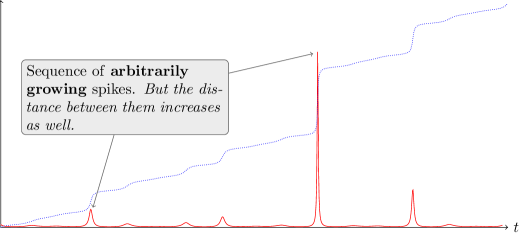
Figure 3. Illustration of $g$ (in dotted blue) from Lemma 3: we start from a function $f$ (in red) that spikes and then integrate it to make it increasing.

[[Ban75]] There exists a positive generable function $g$ and an absolute constant $c>0$ such that for any increasing sequence $a\in\mathbb{N}^{\mathbb{N}}$ with $a_{n}\geqslant 2$ for all $n$, there exists $\alpha\in\mathbb{R}$ such that $g(\alpha,\cdot)$ is defined over $[1,\infty)$, nondecreasing and for any $n\in\mathbb{N}$ and $t\geqslant 2\pi b_{n}$, $g(\alpha,t)\geqslant ca_{n}$ where $b_{n}=\prod_{k=0}^{n-1}a_{k}$. Furthermore, the map $a\mapsto\alpha$ is $(\nu_{\mathbb{N}}^{\omega},\rho)$-computable.

Proof 3.1.

We give a sketch of the proof, following the presentation from [Ban75]. For any $\alpha\in\mathbb{R}$ and $t>0$, let

$$f(\alpha,t)=\frac{1}{2-\cos(t)-\cos(\alpha t)}.$$

Since $\sin$ and $\cos$ are generable, it follows that $f$ is generable because it has a connected domain of definition. Indeed, $f(\alpha,t)$ is well-defined except on

$$X=\left\{(\alpha,2k\pi):\alpha\in\mathbb{Q},k\in\mathbb{N},k\alpha\in\mathbb{N}\right\}$$

which is a totally disconnected set in $\mathbb{R}^{2}$. Let

$$\alpha_{a}=\sum_{n=1}^{\infty}b_{n}^{-1}\qquad\text{where }b_{n}=\prod_{k=0}^{n-1}a_{k}$$ (3)

which is well-defined if $a_{n}$ is a strictly increasing sequence. Indeed, it implies that $b_{n}\geqslant(n-1)!$ and $\alpha_{a}\leqslant\sum_{n=0}^{\infty}\tfrac{1}{n!}=e$. One can easily show (by contradiction for example) that $\alpha_{a}$ must be irrational. Also define

$$g(\alpha,t)=\int_{1}^{t}f(\alpha,u)du$$

which is generable. Let $n\in\mathbb{N}$, define $\delta_{n}=\sum_{k=n+1}^{\infty}\tfrac{b_{n}}{b_{k}}$. Let $t\in[2\pi(b_{n}-\delta_{n}),2\pi b_{n}]$, write $\varepsilon=2\pi b_{n}-t\in[0,2\pi\delta_{n}]$ and observe that

$$1-\cos(t)=1-\cos(t-2\pi b_{n})=1-\cos(\varepsilon)\leqslant\varepsilon^{2}\leqslant 4\pi^{2}\delta_{n}^{2}.$$

Furthermore, and note that

$$1-\cos(\alpha t) =1-\cos(2\pi\alpha b_{n}-\varepsilon)$$

$$=1-\cos\left(2\pi\sum_{k=0}^{n}\tfrac{b_{n}}{b_{k}}+2\pi\sum_{k=n+1}^{\infty}\tfrac{b_{n}}{b_{k}}-\varepsilon\right)$$

$$=1-\cos\left(2\pi\sum_{k=n+1}^{\infty}\tfrac{b_{n}}{b_{k}}-\varepsilon\right) \text{since }\tfrac{b_{n}}{b_{k}}\in\mathbb{N}\text{ for }k\leqslant n$$

$$=1-\cos\left(2\pi\delta_{n}-\varepsilon\right)$$

$$\leqslant\left(2\pi\delta_{n}-\varepsilon\right)^{2} \text{since }1-\cos(x)\leqslant x^{2}$$

$$\leqslant\left(2\pi\delta_{n}\right)^{2} \text{since }\varepsilon\leqslant 2\pi\delta_{n}.$$

It follows that

$$f(\alpha_{a},t)=(1-\cos(t)+1-\cos(\alpha t))^{-1}\geqslant(4\pi^{2}\delta_{n}^{2}+4\pi^{2}\delta_{n}^{2})^{-1}\geqslant\tfrac{1}{8\pi^{2}\delta_{n}^{2}}.$$

Thus

$$g(\alpha_{a},2\pi b_{n}) =\int_{1}^{2\pi b_{n}}f(\alpha_{a},t)dt$$

$$\geqslant\int_{2\pi(b_{n}-\delta_{n})}^{2\pi b_{n}}f(\alpha_{a},t)dt f$$ since is positive

$$\geqslant\int_{2\pi(b_{n}-\delta_{n})}^{2\pi b_{n}}\tfrac{1}{8\pi^{2}\delta_{n}^{2}}dt$$

$$=\tfrac{\delta_{n}}{8\pi^{2}\delta_{n}^{2}}=\tfrac{1}{8\pi^{2}\delta_{n}}.$$

But note that

$$\delta_{n} =\sum_{k=n+1}^{\infty}\tfrac{b_{n}}{b_{k}}\leqslant\sum_{k=n+1}^{\infty}a_{n}^{n-k} \text{since }\tfrac{b_{n}}{b_{k}}=(a_{n}\cdots a_{k-1})^{-1}$$

$$=\frac{a_{n}^{-1}}{1-a_{n}^{-1}}\leqslant 2a_{n}^{-1} \text{since }a_{n}\geqslant 2.$$

It then easily follows that

$$g(\alpha_{a},2\pi b_{n})\geqslant\tfrac{a_{n}}{16\pi^{2}}$$

and the result follows from the fact that $g$ is nondecreasing.

The computability of the map $a\mapsto\alpha$ is the only missing result. It is immediate from (3) that the map $(a,n)\mapsto b_{n}$ is $([\nu_{\mathbb{N}}^{\omega},\nu_{\mathbb{N}}],\nu_{\mathbb{N}})$-computable since each $b_{n}$ is a product of finitely many $a_{i}$. Furthermore, $b_{n}\geqslant(n-1)!$ thus for any $n\geqslant 1$,

$$\left|\alpha_{a}-\sum_{i=1}^{n}b_{i}^{-1}\right|\leqslant\sum_{i\geqslant n-1}\frac{1}{(i-1)!}\leqslant\sum_{i\geqslant n}\frac{1}{i!}\leqslant\sum_{i\geqslant 0}\frac{1}{n!2^{i}}\leqslant\tfrac{2}{n!}\leqslant 2^{2-n}.$$

It follows that $\left(\sum_{i=1}^{n}b_{i}^{-1}\right)_{i\in\mathbb{N}}$ is a Cauchy sequence of $\alpha_{a}$ of known convergence rate. It suffice to note that $(b,n)\mapsto\sum_{i=1}^{n}b_{i}^{-1}$ is $([\nu_{\mathbb{N}}^{\omega},\nu_{\mathbb{N}}],\rho)$-computable, since it only involves a finite number of sum and inverses of real numbers.

Remark 21.

As noted earlier, Lemma 3 and the Theorem 22 build partial functions. Indeed we only show that the solution exists at all times $t\in\mathbb{R}_{\geqslant 0}$ for certain well-chosen $\alpha$. In particular, it can be easily checked that the ODE in Lemma 3 explodes in finite time for all rational $\alpha$.

Essentially, Lemma 3 proves that there exists a function $g$ such that for any $n\in\mathbb{N}$, $g(\alpha,a_{0}a_{1}\cdots a_{n-1})\geqslant a_{n}$. Note that this is not quite what we are aiming for: the function $g$ is indeed $\geqslant a_{n}$ but at times $a_{0}a_{1}\cdots a_{n-1}$ instead of $n$. Since $a_{0}a_{1}\cdots a_{n-1}$ is a very big number compared to $n$, $g$ does not grow fast enough for our needs. The idea is to “accelerate” $g$ by composing it with a fast growing function $h$, ideally such that $h(n)\geqslant a_{0}\cdots a_{n-1}$. This would ensure that $g(h(n))\geqslant n$. This is a chicken-and-egg problem because to build such a function $h$, we need to build a fast growing function! We now try to explain how to solve this problem.

Fix a sequence $(a_{n})_{n}$ and let $g$ be the function from Lemma 3 and $\alpha_{a}$ be the parameter that corresponds to $a$ (we omit the $\alpha_{a}$ for readability so $g(x)=g(\alpha_{a},x)$). Consider the following sequence:

$$x_{0}=a_{0},\qquad x_{n+1}=x_{n}g(x_{n}).$$

Then observe that

$$x_{1}=x_{0}g(x_{0})=a_{0}g(a_{0})\geqslant a_{0}a_{1},\qquad x_{2}=x_{1}g(x_{1})\geqslant a_{0}a_{1}g(a_{0}a_{1})\geqslant a_{0}a_{1}a_{2},\quad\ldots$$

It is not hard to see that $x_{n}\geqslant a_{0}a_{1}\cdots a_{n}\geqslant a_{n}$. We then use our generable gadget of Section 2.2 to simulate this discrete sequence with a differential equation. Intuitively, we build a differential equation such that the solution $y$ satisfies $y(n)\approx x_{n}$. More precisely, we use two variables $y$ and $z$ such that over $[n,n+1/2]$, $z^{\prime}\approx 0$ and $y(t)\rightarrow zg(z)$ and over $[n+1/2,n+1]$, $y^{\prime}\approx 0$ and $z(t)\rightarrow y$. Then if $y(n)\approx z(n)\approx x_{n}$ then $y(n+1)\approx z(n+1)\approx x_{n+1}$.

Theorem 22.

There exists $\Gamma\subseteq\mathbb{R}$ and a positive uniformly-generable function $\mathtt{fastgen}:\Gamma\times\mathbb{R}_{\geqslant 0}\to\mathbb{R}$ such that for any $x\in\mathbb{R}_{\geqslant 0}^{\mathbb{N}}$, there exists $\alpha\in\Gamma$ such that for any $n\in\mathbb{N}$ and $t\in\mathbb{R}_{\geqslant 0}$,

$$\mathtt{fastgen}(\alpha;t)\geqslant x_{n}\qquad\text{if }t\geqslant n.$$

Furthermore, $\mathtt{fastgen}(\alpha;\cdot)$ is nondecreasing. In addition, the map $x\mapsto\alpha$ is $(\rho^{\omega},\rho)$-computable.

Proof 3.2.

Let $\delta=4$. Apply Lemma 3 to get $g$ and $c$. Let $a\in\mathbb{N}^{N}$ be an increasing sequence such that $a_{n}\geqslant x_{n}$, then there exists $\alpha_{x}\in\mathbb{R}$ such that for all $n\in\mathbb{N}$,

$$g(\alpha_{x},t)\geqslant ca_{n}$$ (4)

for all $t\geqslant 2\pi b_{n}$ where $b_{n}=\prod_{k=0}^{n-1}a_{k}$. Consider the following system of differential equations, for $\phi=2$,

$$\left\{\begin{array}[]{@{}r@{\hspace{.25em}}l@{}}y(0)\hskip 2.5pt&=\delta+2\pi\\ z(0)\hskip 2.5pt&=\delta+2\pi\end{array}\right.,\qquad\left\{\begin{array}[]{@{}r@{\hspace{.25em}}l@{}}y^{\prime}(t)\hskip 2.5pt&=\mathtt{pereach}\left(t,\phi,y(t),\delta+\tfrac{1}{c}z(t)g(\alpha_{x},z(t))\right)\\ z^{\prime}(t)\hskip 2.5pt&=\mathtt{pereach}\left(t+\tfrac{1}{2},\phi,z(t),1+y(t)\right)\end{array}\right..$$

Apply Theorem 20 to show that $y$ and $z$ exist over $\mathbb{R}_{\geqslant 0}$. We will show the following result by induction on $n\in\mathbb{N}$:

$$\min(y(n),z(n))\geqslant\delta+2\pi b_{n}.$$ (5)

The result is trivial for $n=0$ since $y(0)=z(0)=\delta+2\pi=\delta+2\pi b_{0}\geqslant 1+2\pi b_{0}$. Let $n\in\mathbb{N}$ and assume that (5) holds for $n$. Apply Theorem 20 (item (iii)) to $z$ to get that for any $t\in[n,n+\tfrac{1}{2}]$,

$$|z(t)-z(n)|\leqslant\int_{n}^{t}\exp\left(-\phi\right)du\leqslant\int_{n}^{n+\tfrac{1}{2}}\exp\left(-\phi\right)du\leqslant\tfrac{1}{2}e^{-\phi}\leqslant 1.$$

In particular, it follows that for any $t\in[n,n+\tfrac{1}{2}]$,

$$z(t) \geqslant z(n)-1\geqslant 2\pi b_{n} \text{since }z(n)\geqslant 1+2\pi b_{n}$$

$$g(\alpha_{x},z(t)) \geqslant ca_{n}$$ using (4)

$$z(t)g(\alpha_{x},z(t)) \geqslant 2\pi b_{n}ca_{n} \text{since }z(t)\geqslant 2\pi b_{n}$$

$$=2\pi cb_{n+1} \text{since }b_{n+1}=b_{n}a_{n}$$

$$\delta+\tfrac{1}{c}z(t)g(\alpha_{x},z(t)) \geqslant\delta+2\pi b_{n+1}.$$

Note that $\phi\geqslant 1$ then apply Theorem 20 (item (iv)) to $y$ using the above inequality to get that

$$y(n+\tfrac{1}{2})\geqslant\delta+2\pi b_{n+1}-e^{-1}\geqslant\delta-1+2\pi b_{n+1}$$

and (item (v)) for any $t\in[n,n+\tfrac{1}{2}]$,

$$y(t)\geqslant\min(y(n),\delta+2\pi b_{n+1})\geqslant\min(1+2\pi b_{n},\delta+2\pi b_{n+1})\geqslant 1+2\pi b_{n},$$ (6)

and (item (iii)) for any $t\in[n+\tfrac{1}{2},n+1]$,

$$|y(t)-y(n+\tfrac{1}{2})|\leqslant\int_{n+\tfrac{1}{2}}^{t}e^{-\phi}du\leqslant\tfrac{e^{-\phi}}{2}\leqslant 1.$$ (7)

Thus $y(t)\geqslant y(n+\tfrac{1}{2})-e^{-1}\geqslant\delta-2-2\pi b_{n+1}$ for any $t\in[n+\tfrac{1}{2},n+1]$. Note that $\phi\geqslant 1$ and apply Theorem 20 (item (iv)) to $z$ using the above inequality to get that

$$z(n+1)\geqslant\min_{u\in[n+\tfrac{1}{2},n+1]}y(u)-e^{-1}\geqslant\delta-2+2\pi b_{n+1}-e^{-1}\geqslant\delta-3+2\pi b_{n+1}.$$

And since $\delta-3\geqslant 1$, we have shown that $y(n+1)$ and $z(n+1)$ are greater than $1+2\pi b_{n+1}$. Furthermore, (6) and (7) prove that for any $t\in[n,n+1]$,

$$y(t)\geqslant\min(1+2\pi b_{n},\delta-2+2\pi b_{n+1})\geqslant 1+2\pi b_{n}.$$

We can thus let $\mathtt{fastgen}(\alpha;t)=y(1+t)$ and get the result since $1+2\pi b_{n+1}\geqslant a_{n}$. Finally, $(\alpha_{x};t)\mapsto y(t)$ is uniformly-generable by Theorem 13 because $\mathtt{pereach}$ and $g$ are generable and the initial condition is computable.

The computability of the map $x\mapsto\alpha$ follows from the computability of the map $a\mapsto\alpha$ (Lemma 3) and the map $x\mapsto a$. Note that the only condition which $a\in\mathbb{N}^{\mathbb{N}}$ has to satisfy is $a_{n}\geqslant x_{n}$. Given a real number represented by its Cauchy sequence, with a known rate of convergence, it is trivial to compute an integer upper bound on this number.

4. Generating a sequence of dyadic rationals

A major part of the proof requires to build a function to approximate arbitrary numbers over intervals $[n,n+1]$. Ideally we would like to build a function that gives $x_{0}$ over $[0,1]$, $x_{1}$ over $[1,2]$, etc. Before we get there, we solve a somewhat simpler problem by making a few assumptions:

• we only try to approximate dyadic numbers, i.e. numbers of the form $m2^{-p}$, and furthermore we only approximate with error $2^{-p-3}$;

• if a dyadic number has size $p$, meaning that it can be written as $m2^{-p}$ but not $m^{\prime}2^{-p+1}$ then it will take a time interval of $p$ units to approximate: $[k,k+p]$ instead of $[k,k+1]$;

• the function will only approximate the dyadics over intervals $[k,k+\tfrac{1}{2}]$ and not $[k,k+1]$.

This processus is illustrated in Figure 4: given a sequence $d_{0},d_{1},\ldots$ of dyadics, there is a corresponding sequence $a_{0},a_{1},\ldots$ of times such that the function approximates $d_{k}$ over $[a_{k},a_{k}+\tfrac{1}{2}]$ within error $2^{-p_{k}}$ where $p_{k}$ is the size of $d_{k}$. The theorem contains an explicit formula for $a_{k}$ that depends on some absolute constant $\delta$.

Figure 4 highlights a feature of $\mathtt{dygen}$: it is an almost piecewise constant function. However we only control the values it takes over small intervals $[a_{i},a_{i}+\tfrac{1}{2}]$, and we have no idea what is the value the rest of the time (even if we know that it is almost piecewise constant).

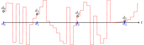
Figure 4. Graph of dygen for $d_{0}=2^{-1}$, $d_{1}=2^{-3}+2^{-1}$, $d_{2}=2^{-5}+2^{-2}$ and $d_{3}=2^{-4}$ (other values ignored) assuming that $\delta=9$. We get that $a_{0}=0$, $a_{1}=10$, $a_{2}=22$, $a_{3}=36$.

Let $\mathbb{D}_{p}=\left\{m2^{-p}:m\in\left\{0,1,\ldots,2^{p}-1\right\}\right\}$ and $\mathbb{D}=\bigcup_{n\in\mathbb{N}}\mathbb{D}_{p}$ denote the set of dyadic rationals in $[0,1)$. For any $q\in\mathbb{D}$, we define its size by $\mathfrak{L}(q)=\min\left\{p\in\mathbb{N}:q\in\mathbb{D}_{p}\right\}$.

Theorem 23.

There exists $\delta\in\mathbb{N}_{>0}$, $\Gamma\subseteq\mathbb{R}^{2}$ and a uniformly-generable function $\mathtt{dygen}:\Gamma\times\mathbb{R}_{\geqslant 0}\to\mathbb{R}$ such that for any dyadic sequence $q\in\mathbb{D}^{\mathbb{N}}$, there exists $(\alpha,\beta)\in\Gamma$ such that for any $n\in\mathbb{N}$,

$$|\mathtt{dygen}(\alpha,\beta;t)-q_{n}|\leqslant 2^{-\mathfrak{L}(q_{n})-3}\qquad\text{for any }t\in[a_{n},a_{n}+\tfrac{1}{2}]$$

where $a_{n}=\sum_{k=0}^{n-1}(\mathfrak{L}(q_{k})+\delta)$. Furthermore, $|\mathtt{dygen}(\alpha,\beta;t)|\leqslant 1$ for all $\alpha,\beta$ and $t$. In addition, the map $q\mapsto(\alpha,\beta)$ is $(\nu_{\mathbb{Q}}^{\omega},[\rho,\rho])$-computable.

Lemma 24.

For any $q\in\mathbb{D}_{p}$, there exists $q^{\prime}\in\mathbb{D}_{p+3}$ such that $|\sin(2q^{\prime}\pi)-q|\leqslant 2^{-p}$ and $|q^{\prime}|\leqslant 1$. Furthermore, $x\mapsto\sin(2\pi x)$ is $8$-Lipschitz. In addition, the map $q\mapsto q^{\prime}$ is ($\nu_{\mathbb{Q}},\nu_{\mathbb{Q}})$-computable.

Proof 4.1.

Let $f(x)=\sin(2\pi x)$ for $x\in[0,\tfrac{1}{4}]$. Clearly $f$ is surjective from $[0,\tfrac{1}{4}]$ to $[0,1]$ thus there exists $x^{\prime}\in[0,\tfrac{1}{4}]$ such that $f(x^{\prime})=q$. Furthermore, since $f^{\prime}(x)=2\pi\cos(2\pi x)$ and $2\pi\leqslant 8$, $f$ is $8$-Lipschitz. Let $q^{\prime}=\lfloor 2^{p+3}x^{\prime}\rfloor 2^{-p-3}$, then $q^{\prime}\in\mathbb{D}_{p+3}$ and $|q^{\prime}-x^{\prime}|\leqslant 2^{-p-3}$ by construction. Clearly $|q^{\prime}|\leqslant 1$, and furthermore,

$$|f(q^{\prime})-q|\leqslant|f(q^{\prime})-f(x^{\prime})|+|f(x^{\prime})-q|\leqslant 8|q^{\prime}-x^{\prime}|+0\leqslant 8\cdot 2^{-p-3}\leqslant 2^{-p}.$$

Note that $f$ is not only surjective from $[0,\tfrac{1}{4}]$ to $[0,1]$ but also increasing and $8$-Lipschitz. Furthermore, $f$ is $(\rho,\rho)$-computable thus a simple dichotomy is enough to find a suitable rational $x^{\prime}$. To conclude, use the fact that the map $x^{\prime}\mapsto q^{\prime}$ is $(\nu_{\mathbb{Q}},\nu_{\mathbb{Q}})$-computable. Note that it is crucial that $x^{\prime}$ is rational because the floor function is not $(\rho,\rho)$-computable.

Proof 4.2 (Proof of Theorem 23).

Let $\delta=9$. Consider the function

$$f(\alpha,t)=\sin\left(2\alpha\pi 2^{t}\right)$$

defined for any $\alpha,t\in\mathbb{R}$. Then $f$ is generable because $\sin$ and $\exp$ are generable. For all $n\in\mathbb{N}$, note that $q_{n}\in\mathbb{D}_{\mathfrak{L}(q_{n})}\subseteq\mathbb{D}_{\mathfrak{L}(q_{n})+\delta-3}$ and apply Lemma 24 to $q_{n}$ to get $q_{n}^{\prime}\in\mathbb{D}_{\mathfrak{L}(q_{n})+\delta}$ such that

$$|\sin(2q_{n}^{\prime}\pi)-q_{n}|\leqslant 2^{-\mathfrak{L}(q_{n})-\delta+3}.$$ (8)

Now define

$$\alpha_{q}=\sum_{k=0}^{\infty}q_{k}^{\prime}2^{-a_{k}}\qquad\text{where }a_{k}=\sum_{\ell=0}^{k-1}(\mathfrak{L}(q_{\ell})+\delta).$$ (9)

It is not hard to see that $\alpha_{q}$ is well-defined (i.e. the sum converges). Let $n\in\mathbb{N}$, then

$$f(\alpha_{q},a_{n}) =\sin(2\pi\alpha_{q}2^{a_{n}})$$

$$=\sin\left(2\pi\sum_{k=0}^{\infty}q_{k}^{\prime}2^{-a_{k}+a_{n}}\right)$$

$$=\sin\left(2\pi\sum_{k=0}^{n-1}q_{k}^{\prime}2^{-a_{k}+a_{n}}+2\pi q_{n}^{\prime}+2\pi\sum_{k=n+1}^{\infty}q_{k}^{\prime}2^{-a_{k}+a_{n}}\right).$$

But for any $k\leqslant n-1$,

$$a_{n}-a_{k}=\sum_{\ell=k}^{n-1}(\mathfrak{L}(q_{\ell})+\delta)\geqslant\mathfrak{L}(q_{k})+\delta$$

and since $q_{k}^{\prime}\in\mathbb{D}_{\mathfrak{L}(q_{k})+\delta}$ and $a_{n}-a_{k}\in\mathbb{N}$, it follows that $q_{k}^{\prime}2^{-a_{k}+a_{n}}\in\mathbb{N}$. Consequently,

$$f(\alpha_{q},a_{n})=\sin\left(2\pi q_{n}^{\prime}+2\pi\sum_{k=n+1}^{\infty}q_{k}^{\prime}2^{-a_{k}+a_{n}}\right)=\sin\left(2\pi(q_{n}^{\prime}+u)\right)$$

where $u=\sum_{k=n+1}^{\infty}q_{k}^{\prime}2^{-a_{k}+a_{n}}$. But for any $k\geqslant n+1$,

$$a_{k}-a_{n}=\sum_{\ell=n}^{k-1}(\mathfrak{L}(q_{\ell})+\delta)\geqslant\mathfrak{L}(q_{n})+\sum_{\ell=n}^{k-1}\delta=\mathfrak{L}(q_{n})+\delta(k-n).$$

Consequently,

$$|u|\leqslant\sum_{k=n+1}^{\infty}|q_{k}^{\prime}|2^{-a_{k}+a_{n}}\leqslant\sum_{k=n+1}^{\infty}2^{-\mathfrak{L}(q_{n})-\delta(k-n)}\leqslant 2^{-\mathfrak{L}(q_{n})}\sum_{k=1}^{\infty}2^{-\delta k}\leqslant 2^{-\mathfrak{L}(q_{n})-\delta+1}.$$

Since $x\mapsto\sin(2\pi x)$ is $8$-Lipschitz, it follows that

$$|f(\alpha_{q},a_{n})-q_{n}| =|\sin\left(2\pi(q_{n}^{\prime}+u)\right)-q_{n}|$$

$$\leqslant|\sin\left(2\pi(q_{n}^{\prime}+u)\right)-\sin(2\pi q_{n}^{\prime})|+|\sin(2q_{n}^{\prime}\pi)-q_{n}|$$

$$\leqslant 8|u|+2^{-\mathfrak{L}(q_{n})-\delta+3}$$ using (8)

$$\leqslant 8\cdot 2^{-\mathfrak{L}(q_{n})-\delta+1}+2^{-\mathfrak{L}(q_{n})-\delta+3}$$

$$\leqslant 2^{-\mathfrak{L}(q_{n})-\delta+5}.$$ (10)

Recall that $\mathtt{round}$ is the generable rounding function from Lemma 16, and fastgen the fast growing function from Theorem 22. Let $\alpha,\beta,t\in\mathbb{R}$, if $\mathtt{fastgen}(\beta;t)$ exists then let

$$\mathtt{dygen}(\alpha,\beta;t)=f(\alpha,r(\beta;t))$$

where

$$r(\beta;t)=\mathtt{round}\left(t-\tfrac{1}{4},\mathtt{fastgen}(\beta;t)\ln 2,4\right).$$

Note that dygen is uniformly-generable because $f,\mathtt{round}$ and fastgen are uniformly-generable. Apply Theorem 22 to get $\beta_{q}\in\mathbb{R}$ such that for any $n\in\mathbb{N}$ and $t\in\mathbb{R}_{\geqslant 0}$,

$$\mathtt{fastgen}(\beta_{q};t)\geqslant a_{n}+\mathfrak{L}(q_{n})+\delta\qquad\text{if }t\in[a_{n},a_{n}+1).$$

Let $n\in\mathbb{N}$ and $t\in[a_{n},a_{n}+\tfrac{1}{2}]$, then $t-\tfrac{1}{4}\in\left[a_{n}-\tfrac{1}{2}+\tfrac{1}{\lambda},a_{n}+\tfrac{1}{2}-\tfrac{1}{\lambda}\right]$ for $\lambda=4$. Thus we can apply Lemma 16 and get that

$$|r(\beta_{q},t)-a_{n}|\leqslant e^{-\mathtt{fastgen}(\beta_{q};t)\ln 2}=2^{-\mathtt{fastgen}(\beta_{q};t)}\leqslant 2^{-a_{n}-\mathfrak{L}(q_{n})-\delta}\leqslant 1.$$ (11)

Observe that

$$\left|\tfrac{\partial f}{\partial t}(\alpha_{q},t)\right|=2\pi|\alpha_{q}|2^{t}|\cos(2\alpha_{q}\pi 2^{t})|\leqslant 2\pi 2^{t}\leqslant 2^{t+3}.$$

Thus for any $t,t^{\prime}\in\mathbb{R}$,

$$|f(\alpha_{q},t)-f(\alpha_{q},t^{\prime})|\leqslant 2^{3+\max(t,t^{\prime})}|t-t^{\prime}|.$$

It follows that for any $n\in\mathbb{N}$ and $t\in[a_{n},a_{n}+\tfrac{1}{2}]$,

$$|\mathtt{dygen}(\alpha_{q},\beta_{q};t)-q_{n}| =|f(\alpha_{q},r(\beta_{q};t))-q_{n}|$$

$$\leqslant|f(\alpha_{q},r(\beta_{q};t))-f(\alpha_{q},a_{n})|+|f(\alpha_{q},a_{n})-q_{n}|$$

$$\leqslant 2^{3+\max(a_{n},r(\beta_{q};t))}|r(\beta_{q};t)-a_{n}|+2^{-\mathfrak{L}(q_{n})-3}$$ using (10)

$$\leqslant 2^{3+a_{n}+1}2^{-\mathfrak{L}(q_{n})-a_{n}-\delta}+2^{-\mathfrak{L}(q_{n})-\delta+5}$$ using (11)

$$\leqslant 2^{-\mathfrak{L}(q_{n})-\delta+4}+2^{-\mathfrak{L}(q_{n})-\delta+5}$$

$$\leqslant 2^{-\mathfrak{L}(q_{n})-\delta+6}$$

$$\leqslant 2^{-\mathfrak{L}(q_{n})-3} \text{since }\delta-6\geqslant 3.$$

To see that the map $q\mapsto(\alpha_{q},\beta_{q})$ is computable, first note that the map $q_{n}\mapsto q_{n}^{\prime}$ is computable (Lemma 24), thus the map $q\mapsto q^{\prime}$ is $(\nu_{\mathbb{Q}}^{\omega},\nu_{\mathbb{Q}}^{\omega})$-computable. It is clear from (9) that $q^{\prime}\mapsto a$ is also computable. Using a similar argument as above, one can easily see that the partial sums (of the infinite sum) defining $\alpha_{q}$ in (9) form a Cauchy sequence with convergence rate $k\mapsto 2^{-k}$ because $a_{k}\geqslant k\delta\geqslant k$. Finally, $q\mapsto\beta_{q}$ is computable by Theorem 22.

5. Generating a sequences of bits

We saw in the previous section how to generate a dyadic generator. Unfortunately, we saw that it generates dyadic $d_{n}$ at times $a_{n}$, whereas we would like to get $d_{n}$ at time $n$ for our approximation. Our approach is to build a signal generator that will be high exactly at times $a_{n}$. Each time the signal will be high, the system will copy the value of the dyadic generator to a variable and wait until the next signal. Since the signal is binary, we only need to generate a sequence of bits. Note that this theorem has a different flavour from the dyadic generator: it generates a more restrictive set of values (bits) but does so much better because we have control over the timing and we can approximate the bits with arbitrary precision.

Figure 5 shows what $\mathtt{bitgen}$ looks like: it is an almost piecewise constant function such that the value in the interval $[n,n+\tfrac{1}{2}]$ is almost the $n^{th}$ digit of $\alpha$.

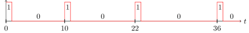
Figure 5. (Ideal) graph of $\mathtt{bitgen}$ for $b\in\left\{0,1\right\}^{\mathbb{N}}$ where $b_{0}=b_{10}=b_{22}=b_{36}=1$ and all the other bits are $0$.

Remark 25.

Although it is possible to define bitgen using dygen, it does not, in fact, give a shorter proof but definitely gives a more complicated function.

Theorem 26.

There exists $\Gamma\subseteq\mathbb{R}$ and a generable function $\mathtt{bitgen}:\Gamma\times\mathbb{R}_{\geqslant 0}^{2}\to\mathbb{R}$ such that for any bit sequence $b\in\left\{0,1\right\}^{\mathbb{N}}$, there exists $\alpha_{b}\in\Gamma$ such that for any $\mu\in\mathbb{R}_{\geqslant 0}$, $n\in\mathbb{N}$ and $t\in[n,n+\tfrac{1}{2}]$,

$$|\mathtt{bitgen}(\alpha_{b},\mu,t)-b_{n}|\leqslant e^{-\mu}.$$

Furthermore, $|\mathtt{bitgen}(\alpha,\mu,t)|\leqslant 1$ for all $\alpha,\mu$ and $t$. Finally, the map $b\mapsto\alpha_{b}$ is $(\nu_{\mathbb{N}}^{\omega},\rho)$-computable.

Proof 5.1.

Consider the function

$$f(\alpha,t)=\sin\left(2\pi\alpha 4^{t}+\tfrac{4\pi}{3}\right)$$

defined for any $\alpha,t\in\mathbb{R}$. Then $f$ is generable because $\sin$ and $\exp$ are generable. For any $b\in\left\{0,1\right\}^{\mathbb{N}}$, let

$$\alpha_{b}=\sum_{k=0}^{\infty}2b_{k}4^{-k-1}.$$ (12)

Let $b\in\left\{0,1\right\}^{\mathbb{N}}$ and $n\in\mathbb{N}$, observe that

$$f(\alpha_{b},n) =\sin\left(2\pi\sum_{k=0}^{\infty}2b_{k}4^{-k-1}4^{n}+\tfrac{4\pi}{3}\right)$$

$$=\sin\left(2\pi\underbrace{\sum_{k=0}^{n-1}2b_{k}4^{n-k-1}}_{\in\mathbb{N}}+2\pi 2b_{n}4^{-1}+2\pi\sum_{k=n+1}^{\infty}2b_{k}4^{n-k-1}+\tfrac{4\pi}{3}\right)$$

$$=\sin\left(\pi b_{n}+\tfrac{4\pi}{3}+\delta\right)$$

where

$$\delta=2\pi\sum_{k=n+1}^{\infty}2b_{k}4^{n-k-1}=4\pi\sum_{k=0}^{\infty}b_{k}4^{-k-2}\leqslant 4\pi\sum_{k=0}^{\infty}4^{-k-2}=4\pi\tfrac{4^{-2}}{3}=\frac{\pi}{3}.$$

It follows that if $b_{n}=0$ then $\pi b_{n}+\tfrac{4\pi}{3}+\varepsilon\in\left[\tfrac{4\pi}{3},\tfrac{5\pi}{3}\right]$ and if $b_{n}=1$ then $\pi b_{n}+\tfrac{4\pi}{3}+\varepsilon\in\left[\tfrac{7\pi}{3},\tfrac{8\pi}{3}\right]$. Thus

$$f(\alpha_{b},n)\in\left[-1,-\tfrac{\sqrt{3}}{2}\right]\text{ if }b_{n}=0,\qquad\qquad f(\alpha_{b},n)\in\left[\tfrac{\sqrt{3}}{2},1\right]\text{ if }b_{n}=1.$$ (13)

Furthermore,

$$|\alpha_{b}|=\sum_{k=0}^{\infty}2b_{k}4^{-k-1}\leqslant\tfrac{2}{4}\sum_{k=0}^{\infty}4^{-k}\leqslant\tfrac{2}{3}.$$ (14)

Let $\varepsilon\in\left[-\tfrac{1}{2},\tfrac{1}{2}\right]$, then for any $t\in\mathbb{R}$,

$$|f(\alpha_{b},t+\varepsilon)-f(\alpha_{b},t)| =\left|\sin\left(2\pi\alpha_{b}4^{t+\varepsilon}+\tfrac{4\pi}{3}\right)-\sin\left(2\pi\alpha_{b}4^{t}+\tfrac{4\pi}{3}\right)\right|$$

$$=\left|2\cos(2\pi\alpha_{b}(4^{t}+4^{t+\varepsilon})+\tfrac{8\pi}{3})\sin\left(2\pi\alpha_{b}(4^{t+\varepsilon}-4^{t})\right)\right|$$

$$\leqslant 2|\sin(2\pi\alpha_{b}(4^{t+\varepsilon}-4^{t}))|$$

$$\leqslant 4\pi|\alpha_{b}||4^{t+\varepsilon}-4^{t}|$$

$$\leqslant 4\pi\frac{2}{3}4^{t}|4^{\varepsilon}-1|$$ using (14)

$$\leqslant\frac{8\pi}{3}4^{t}2\varepsilon \text{using that }|\varepsilon|\leqslant\tfrac{1}{2}$$

$$\leqslant 4^{t}B\varepsilon$$ (15)

for some constant $B>0$. Recall that $\mathtt{round}$ is the generable rounding function from Lemma 16. Let $\alpha,t\in\mathbb{R}$, $\mu\in\mathbb{R}_{\geqslant 0}$ and define

$$g(\alpha,t)=f(\alpha,r(t))\quad\text{where}\quad r(t)=\mathtt{round}(t-\tfrac{1}{4},t\ln 4+\ln B,4).$$

Note again that $g$ is generable because $f$ and $\mathtt{round}$ are generable. Let $n\in\mathbb{N}$ and $t\in[n,n+\tfrac{1}{2}]$, then $t-\tfrac{1}{4}\in\left[n-\tfrac{1}{4},n+\tfrac{3}{4}\right]=\left[n-\tfrac{1}{4}+\tfrac{1}{\lambda},n+\tfrac{1}{2}-\tfrac{1}{\lambda}\right]$ for $\lambda=4$. Thus we can apply Lemma 16 and get that

$$|r(t)-n|\leqslant e^{-(n+1)\ln 4+\ln B}=\tfrac{4^{-n-1}}{B}.$$

It follows using (15) that

$$|g(\alpha_{b},t)-f(\alpha_{b},n)|=|f(\alpha_{b},r(t))-f(\alpha_{b},n)|\leqslant 4^{t}B\tfrac{4^{-n-1}}{B}=\tfrac{1}{4}.$$

And since $\tfrac{\sqrt{3}}{2}-\tfrac{1}{4}\geqslant\tfrac{1}{2}$, we conclude using (13) that for any $t\in\left[n,n+\tfrac{1}{2}\right]$,

$$g(\alpha_{b},t)\in\left[-1,-\tfrac{1}{2}\right]\text{ if }b_{n}=0,\qquad\qquad g(\alpha_{b},t)\in\left[\tfrac{1}{2},1\right]\text{ if }b_{n}=1.$$ (16)

Finally, let $\alpha,t\in\mathbb{R}$, $\mu\in\mathbb{R}_{\geqslant 0}$ and define

$$\mathtt{bitgen}(\alpha,\mu\,t)=\frac{1+\tanh(2\mu g(\alpha,t))}{2}.$$

Note that bitgen is generable because $\tanh$ and $g$ are generable. Let $\mu\in\mathbb{R}_{\geqslant 0}$, $n\in\mathbb{N}$ and $t\in\left[n,n+\tfrac{1}{2}\right]$. If $b_{n}=0$, then it follows from (16) that

$$g(\alpha_{b},n) \leqslant-\tfrac{1}{2}$$

$$|\tanh(2\mu g(\alpha_{b},n))-\mathtt{sgn}(2\mu g(\alpha_{b},n))| \leqslant e^{-2\mu|g(\alpha_{b},n)|}$$ using Lemma 17

$$|\tanh(2\mu g(\alpha_{b},n))+1| \leqslant e^{-\mu}$$

$$|\mathtt{bitgen}(\alpha_{b},\mu,t)-b_{n}| \leqslant\tfrac{1}{2}e^{-\mu}\leqslant e^{-\mu} \text{since }b_{n}=0.$$

Similarly, if $b_{n}=1$, then

$$g(\alpha_{b},n) \geqslant\tfrac{1}{2}$$

$$|\tanh(2\mu g(\alpha_{b},n))-\mathtt{sgn}(2\mu g(\alpha_{b},n))| \leqslant e^{-2\mu|g(\alpha_{b},n)|}$$

$$|\tanh(2\mu g(\alpha_{b},n))-1| \leqslant e^{-\mu}$$

$$|\mathtt{bitgen}(\alpha_{b},\mu,t)-b_{n}| \leqslant\tfrac{1}{2}e^{-\mu}\leqslant e^{-\mu} \text{since }b_{n}=1.$$

Finally, it is clear from (12) that the partial sums are easily computable and form a Cauchy sequence that converges at rate $4^{-k}$, thus $\alpha_{b}$ is computable from $b$.

6. Generating an almost piecewise constant function

We have already explained the main intuition of this section in previous sections. Using the dyadic generator and the bit generator as a signal, we can construct a system that “samples” the dyadic at the right time and then holds this value still until the next dyadic. In essence, we just described an almost piecewise constant function. This function still has a limitation: its rate of change is small so it can only approximate slowly changing functions. Figure 6 illustrates how this process works at the high-level.

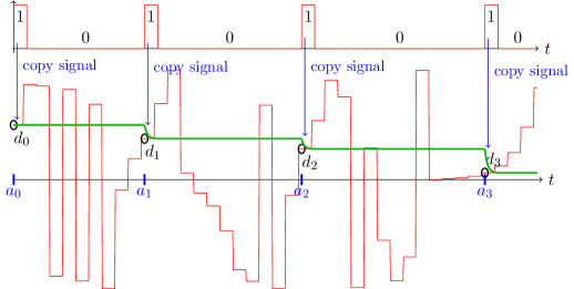
Figure 6. Illustration of the process to generate an almost piecewise-constant function: $\mathtt{bitgen}$ is used to generate a copy signal, which we synchronise with $\mathtt{dygen}$ to copy exactly the sequence of dyadic numbers we specified. In-between copies, we ensure that copied value does not change (sample and hold).

Theorem 27.

There exists an absolute constant $\delta\in\mathbb{N}$, $p\in\mathbb{N}$, $\Gamma\subseteq\mathbb{R}^{p}$ and a uniformly-generable function $\mathtt{pwcgen}:\Gamma\times\mathbb{R}_{\geqslant 0}\to\mathbb{R}$ such that for any dyadic sequence $q\in\mathbb{D}^{\mathbb{N}}$, there exists $\alpha_{q}\in\Gamma$ such that for any $n\in\mathbb{N}$, putting $a_{n}=\sum_{k=0}^{n-1}(\delta+\mathfrak{L}(q_{k}))$, we have that

$$|\mathtt{pwcgen}(\alpha_{q};t)-q_{n}|\leqslant 2^{-\mathfrak{L}(q_{n})}\qquad\text{for any }t\in[a_{n}+\tfrac{1}{2},a_{n+1}]$$

and $\mathtt{pwcgen}(\alpha_{q};t)\in I_{n}$ for any $t\in[a_{n},a_{n}+\tfrac{1}{2}]$ where

$$I_{n}:=\left[\mathtt{pwcgen}(\alpha_{q};a_{n}),\mathtt{pwcgen}(\alpha_{q};a_{n}+\tfrac{1}{2})\right]+2^{-\mathfrak{L}(q_{n})}[-1,1].$$

Finally, the map $q\mapsto\alpha_{q}$ is $(\nu_{\mathbb{Q}}^{\omega},\rho^{p})$-computable.

Proof 6.1.

Apply Theorem 23 to get $\delta\in\mathbb{N}$, dygen uniformly-generable, and $\alpha_{q},\beta_{q}$ such that for any $n\in\mathbb{N}$,

$$|\mathtt{dygen}(\alpha_{q},\beta_{q};t)-q_{n}|\leqslant 2^{-\mathfrak{L}(q_{n})-3}\qquad\text{for any }t\in[a_{n},a_{n}+\tfrac{1}{2}]$$

where $a_{n}=\sum_{k=0}^{n-1}(\mathfrak{L}(q_{k})+\delta)$. Let $b\in\left\{0,1\right\}^{\mathbb{N}}$ be the bit sequence defined by

$$b_{n}=\begin{cases}1&\text{if }n=a_{k}\text{ for some }k\\ 0&\text{otherwise.}\end{cases}$$

Apply Theorem 26 to get bitgen and $\gamma_{b}$ such that for any $\mu\in\mathbb{R}_{\geqslant 0}$, $n\in\mathbb{N}$ and $t\in[n,n+\tfrac{1}{2}]$,

$$|\mathtt{bitgen}(\gamma_{b},\mu,t)-b_{n}|\leqslant e^{-\mu}.$$

Let $x_{n}=\mathfrak{L}(q_{n})+3$ and apply Theorem 22 to get $\lambda_{a}$ and fastgen such that for any $n\in\mathbb{N}$,

$$\mathtt{fastgen}(\lambda_{a};t)\geqslant x_{n}\qquad\text{for all }t\in[n,n+1].$$

Consider the following system for all $t\in\mathbb{R}_{\geqslant 0}$:

$$y(0)=q_{0},\qquad y^{\prime}(t)=\psi(t)r(t),\qquad r(t)=\mathtt{pereach}(t,\phi(t),y(t),g(t))$$

where

$$\phi(t)=t+\mathtt{fastgen}(\lambda_{a};t),\qquad\psi(t)=2\mathtt{bitgen}(\gamma_{b},\phi(t)+R(t),t),$$

$$g(t)=\mathtt{dygen}(\alpha_{q},\beta_{q};t),\qquad R(t)=1+r(t)^{2}.$$

We omitted the parameters $\alpha,\beta,\gamma,\lambda$ in the functions $g$ and $\phi$ to make it more readable. It is clear that $g$ and $\phi$ are uniformly-generable since $\texttt{bitgen},\texttt{fastgen},\texttt{dygen}$ are uniformly-generable. It follows that $(q_{0},\alpha,\beta,\gamma,\lambda,t)\mapsto y(t)$ is also uniformly-generable by Theorem 13. Indeed, the only extra thing we need to check is that the initial condition is a computable function of the parameters, which it is since we just need to extract $q_{0}$ from the list of parameters.

We will show the result by induction. Let $n\in\mathbb{N}$ and assume that $|y(a_{n})-q_{n}|\leqslant 2^{-x_{n}}$. Note that this is trivially satisfied for $n=0$ since $a_{0}=0$ and thus $y(a_{0})=y(0)=q_{0}$. We will now do the analysis of the behavior of $y$ over $[a_{n},a_{n+1}]$ by making a case distinction between $[a_{n},a_{n}+1]$ and $[a_{n}+1,a_{n+1}]$. Note that for all $t$, $R(t)\geqslant|r(t)|\geqslant 0$.

When $\mathbf{t\in[a_{n},a_{n}+\tfrac{1}{2}]}$, we have that

$$|\mathtt{bitgen}(\gamma_{b},\mu,t)-b_{a_{n}}|\leqslant e^{-\mu}$$

but $b_{a_{n}}=1$ by definition thus

$$\mathtt{bitgen}(\gamma_{b},\phi(t)+R(t),t)\geqslant 1-e^{-\phi(t)}\geqslant\tfrac{1}{2}$$

since $\phi(t)\geqslant\mathtt{fastgen}(\lambda_{a};t)\geqslant 1$. Furthermore,

$$\phi(t)\geqslant\mathtt{fastgen}(\lambda_{a};t)\geqslant\mathtt{fastgen}(\lambda;n)\geqslant x_{n}\geqslant 2.$$

Thus $\psi(t)\phi(t)=2\mathtt{bitgen}(\gamma_{b},\phi(t)+R(t),t)\phi(t)\geqslant x_{n}\geqslant 2$. Furthermore,

$$|g(t)-q_{n}|=|\mathtt{dygen}(\alpha_{q},\beta_{q};t)-q_{n}|\leqslant 2^{-x_{n}}$$ (17)

thus we can apply Theorem 20 to get the existence of $y$ and item (i) to get that

$$|y(a_{n}+\tfrac{1}{2})-q_{n}|\leqslant 2^{-x_{n}}+e^{-x_{n}}\leqslant 2^{-x_{n}+1}.$$ (18)

Note that (17) implies that

$$q_{n}-2^{-x_{n}}\leqslant g(t)\leqslant q_{n}+2^{-x_{n}}$$

and thus (18) proves that

$$y(a_{n}+\tfrac{1}{2})-2^{-x_{n}+1}\leqslant q_{n}\leqslant y(a_{n}+\tfrac{1}{2})+2^{-x_{n}+1}.$$ (19)

Furthermore, Theorem 20 item (v) also gives us that

$$\min(y(a_{n}),q_{n}-2^{-x}) \leqslant y(t)\leqslant\max(y(a_{n}),q_{n}+2^{-x_{n}})$$

$$\min(y(a_{n}),y(a_{n}+\tfrac{1}{2})-3\cdot 2^{-x_{n}}) \leqslant y(t)\leqslant\max(y(a_{n}),y(a_{n}+\tfrac{1}{2})+3\cdot 2^{-x_{n}})$$ using (19)

$$y(t)\in[y(a_{n}),y(a_{n}+\tfrac{1}{2})]+[-3\cdot 2^{-x_{n}},3\cdot 2^{-x_{n}}]$$

$$y(t)\in[y(a_{n}),y(a_{n}+\tfrac{1}{2})]+[-2^{-\mathfrak{L}(q_{n})},2^{-\mathfrak{L}(q_{n})}].$$ (20)

When $\mathbf{t\in[a_{n}+k+\tfrac{1}{2},a_{n}+k+1]}$ for $\mathbf{a_{n}\leqslant a_{n}+k<a_{n+1}}$, we have that

$$y^{\prime}(t)=\psi(t)\mathtt{pereach}(t,\phi(t),y(t),g(t))$$

where $|\psi(t)|\leqslant 2$ since $|\mathtt{bitgen}|\leqslant 1$ by Theorem 26 and

$$\phi(t)\geqslant t+\mathtt{fastgen}(\lambda_{a};t)\geqslant t+\mathtt{fastgen}(\lambda;n)\geqslant t+x_{n}.$$

Thus by Theorem 20 item (iii) we have that

$$|y(t)-y(a_{n}+k+\tfrac{1}{2})|\leqslant\int_{a_{n}+k+\tfrac{1}{2}}^{t}\psi(u)\exp(-\phi(u))du\leqslant\tfrac{1}{2}2e^{-x_{n}}\int_{a_{n}+k+\tfrac{1}{2}}^{t}e^{-u}du.$$

When $\mathbf{t\in[a_{n}+k,a_{n}+k+\tfrac{1}{2}]}$ for $\mathbf{a_{n}<a_{n}+k<a_{n+1}}$, we have that

$$|\mathtt{bitgen}(\gamma_{b},\mu,t)-b_{a_{n}+k}|\leqslant e^{-\mu}$$

but $b_{a_{n}+k}=0$ by definition thus

$$|\mathtt{bitgen}(\gamma_{b},\phi(t)+R(t),t)|\leqslant e^{-\phi(t)-R(t)}.$$

Furthermore,

$$\phi(t)\geqslant t+\mathtt{fastgen}(\lambda_{a};t)\geqslant t+\mathtt{fastgen}(\lambda;n)\geqslant t+x_{n}.$$

Thus

$$|\psi(t)|=2|\mathtt{bitgen}(\gamma_{b},\phi(t)+R(t),t)|\leqslant 2e^{-t-x_{n}}e^{-R(t)}\leqslant 2e^{-t-x_{n}}e^{-|r(t)|}.$$

It follows that

$$y^{\prime}(t)=\psi(t)r(t)$$

where

$$|\psi(t)r(t)|\leqslant 2e^{-\phi(t)-R(t)}|r(t)|\leqslant 2e^{-t-x_{n}}.$$

Consequently,

$$|y(t)-y(a_{n}+k)|\leqslant\int_{a_{n}+k}^{a_{n}+k+\tfrac{1}{2}}|\psi(u)r(u)|du\leqslant e^{-x_{n}}\int_{a_{n}+k}^{a_{n}+k+\tfrac{1}{2}}e^{-u}du.$$

Putting everything together we get that for all $t\in[a_{n}+\tfrac{1}{2},a_{n+1}]$,

$$|y(t)-y(a_{n}+\tfrac{1}{2})|\leqslant e^{-x_{n}}\int_{a_{n}+1}^{t}e^{-u}du\leqslant e^{-x_{n}}$$

and thus using (18), for all $t\in[a_{n}+\tfrac{1}{2},a_{n+1}]$,

$$|y(t)-q_{n}|\leqslant e^{-x_{n}}+|y(a_{n}+\tfrac{1}{2})-q_{n}|\leqslant e^{-x_{n}}+2^{-x_{n}+1}\leqslant 2^{-x_{n}+2}\leqslant 2^{-\mathfrak{L}(q_{n})}.$$

Also recall (20) that for all $t\in[a_{n},a_{n}+\tfrac{1}{2}]$,

$$y(t)\in[y(a_{n}),y(a_{n}+\tfrac{1}{2})]+[-2^{-\mathfrak{L}(q_{n})},2^{-\mathfrak{L}(q_{n})}].$$

We have already shown that the map $Y(q_{0},\alpha_{q},\beta_{q},\gamma_{q},\lambda_{a},t)=y(t)$ is uniformly-generable. Finally, we need to show computability of the map $q\mapsto(\alpha_{q},\beta_{q},\gamma_{b},\lambda_{a})$. Computability of $\alpha_{q}$ and $\beta_{q}$ follows from Theorem 23. The sequence $(a_{n})_{n}$, and thus $(b_{n})_{n}$, is easily computed from $q$. It follows that from Theorem 26 that $\gamma_{b}$ is computable from $b$, and from Theorem 22 that $\lambda_{a}$ is computable from $a$.

7. Proof of the main theorem

The proof works in several steps. First we show that using an almost constant function, we can approximate functions that are bounded and change very slowly. We then relax all these constraints until we get to the general case. In the following, we only consider total functions over $\mathbb{R}$. See Remark on page 6 for more details.

[Universality] Let $I\subseteq\mathbb{R}$ and $\mathcal{C}\subseteq C^{0}(I)\times C^{0}(I,\mathbb{R}_{>0})$. We say that the universality property holds for $\mathcal{C}$ if there exists $d\in\mathbb{N}$, $\Gamma\subseteq\mathbb{R}^{d}$ and a uniformly-generable function $\mathfrak{u}:\Gamma\times I\to\mathbb{R}$ such that for every $(f,\varepsilon)\in\mathcal{C}$, there exists $\alpha\in\Gamma$ such that

$$|\mathfrak{u}(\alpha;t)-f(t)|\leqslant\varepsilon(t)\qquad\text{for all }t\in I.$$

The universality property is said to be effective if furthermore the map $(f,\varepsilon)\mapsto\alpha$ is $([\rho\to\rho]^{2},\rho^{d})$-computable.

Lemma 28.

There exists a constant $c>0$ such that the universality property holds for all $(f,\varepsilon)$ on $\mathbb{R}_{\geqslant 0}$ such that for all $t\in\mathbb{R}_{\geqslant 0}$:

• $\varepsilon$ is decreasing and $-\log_{2}\varepsilon(t)\leqslant c^{\prime}+t$ for some constant $c^{\prime}$,

• $f(t)\in[0,1]$,

• $|f(t)-f(t^{\prime})|\leqslant c\varepsilon(t+1)$ for all $t^{\prime}\in[t,t+1]$.

Furthermore, the universality property is effective for this class.

Proof 7.1 (Proof Sketch).

This is essentially a application of pwcgen with a small twist. Indeed the bound on $f$ guarantees that dyadic rationals are enough. The bound on the rate of change of $f$ guarantees that a single dyadic can provide an approximation for a long enough time. And the bound on $\varepsilon$ guarantees that we do not need too many digits for the approximations.

Proof 7.2.

Let $c=\tfrac{1}{8}$. Apply Theorem 27 to get $p,\delta\in\mathbb{N}$ and pwcgen. Let $f$ and $\varepsilon$ be as described in the statement. For any $n\in\mathbb{N}$, let $q_{n}\in\mathbb{D}$ be such that

$$|f(n)-q_{n}|\leqslant 2^{-\mathfrak{L}(q_{n})}\leqslant c\varepsilon(n+1).$$ (21)

Since by assumption, $-\log_{2}\varepsilon(n+1)\leqslant c^{\prime}+n+1$, we can always choose $q_{n}$ so that

$$\mathfrak{L}(q_{n})=\left\lceil c^{\prime}\right\rceil+n+1.$$

Then by Theorem 27, there exists $\alpha_{q}\in\mathbb{R}^{p}$ such that

$$|\mathtt{pwcgen}(\alpha_{q};t)-q_{n}|\leqslant 2^{-\mathfrak{L}(q_{n})}\qquad\text{for any }t\in[a_{n}+\tfrac{1}{2},a_{n+1}]$$

and

$$\mathtt{pwcgen}(\alpha_{q};t)\in\left[\mathtt{pwcgen}(\alpha_{q};a_{n}),\mathtt{pwcgen}(\alpha_{q};a_{n}+\tfrac{1}{2})\right]\qquad\text{for any }t\in[a_{n},a_{n}+\tfrac{1}{2}]$$ (22)

where

$$a_{n}=\sum_{k=0}^{n-1}(\delta+\mathfrak{L}(q_{k}))=\sum_{k=0}^{n-1}(\delta+\left\lceil c^{\prime}\right\rceil+n+1)=n(\delta+\left\lceil c^{\prime}\right\rceil+1)+\tfrac{1}{2}n(n-1).$$

Introduce the function

$$\xi(t)=t(\delta+\left\lceil c^{\prime}\right\rceil+1)+\tfrac{1}{2}t(t-1)$$

so that $a_{n}=\xi(n)$ and note that $\xi$ is increasing and generable. Let $t\in[\xi^{-1}(a_{n}+\tfrac{1}{2}),\xi^{-1}(a_{n+1})]$, since $\xi$ is increasing, so is $\xi^{-1}$ and

$$n=\xi^{-1}(a_{n})\leqslant\xi^{-1}(a_{n}+\tfrac{1}{2})\leqslant t\leqslant\xi^{-1}(a_{n+1})=n+1.$$

So in particular,

$$|f(n)-f(t)|\leqslant c\varepsilon(n+1)$$

by the assumption on $f$, since $t\in[n,n+1]$. It follows that

$$|\mathtt{pwcgen}(\alpha_{q};\xi(t))-f(t)| \leqslant|\mathtt{pwcgen}(\alpha_{q};\xi(t))-q_{n}|$$

$$\hskip 8.5359pt+|q_{n}-f(n)|+|f(n)-f(t)|$$

$$\leqslant 2^{-\mathfrak{L}(q_{n})}+2^{-\mathfrak{L}(q_{n})}+c\varepsilon(n+1) \text{since }\xi(t)\in[a_{n}+\tfrac{1}{2},a_{n+1}]$$

$$\leqslant 3c\varepsilon(n+1)$$

$$\leqslant 3c\varepsilon(t) \varepsilon$$ since is decreasing

$$\leqslant\varepsilon(t) \text{since }3c\leqslant 1.$$

So in particular, in implies that for all $n\in\mathbb{N}$,

$$|\mathtt{pwcgen}(\alpha_{q};a_{n}+\tfrac{1}{2})-f(\xi^{-1}(a_{n}+\tfrac{1}{2}))|\leqslant 3c\varepsilon(n+1)$$ (23)

and

$$|\mathtt{pwcgen}(\alpha_{q};a_{n+1})-f(n+1)|\leqslant 3c\varepsilon(n+2).$$ (24)

Let $t\in[\xi^{-1}(a_{n+1}),\xi^{-1}(a_{n+1}+\tfrac{1}{2})]$, it follows using (22) that there exists $\lambda\in[0,1]$ such that

$$\mathtt{pwcgen}(\alpha_{q};\xi(t))=\lambda\mathtt{pwcgen}(\alpha_{q};a_{n+1})+(1-\lambda)\mathtt{pwcgen}(\alpha_{q};a_{n+1}+\tfrac{1}{2}).$$

We also have that

$$n+1=\xi^{-1}(a_{n+1})\leqslant t\leqslant\xi^{-1}(a_{n+1}+\tfrac{1}{2})\leqslant\xi^{-1}(a_{n+2})=n+2.$$

Thus

$$|\mathtt{pwcgen}(\alpha_{q};\xi(t))-f(t)| \leqslant\lambda|\mathtt{pwcgen}(\alpha_{q};a_{n+1})-f(t)|$$

$$\hskip 20.00003pt+(1-\lambda)|\mathtt{pwcgen}(\alpha_{q};a_{n+1}+\tfrac{1}{2})-f(t)|$$

$$\leqslant|\mathtt{pwcgen}(\alpha_{q};a_{n+1})-f(n+1)|+|f(n+1)-f(t)|$$

$$\hskip 20.00003pt+|\mathtt{pwcgen}(\alpha_{q};a_{n+1}+\tfrac{1}{2})-f(\xi^{-1}(a_{n+1}+\tfrac{1}{2}))|$$

$$\hskip 20.00003pt+|f(\xi^{-1}(a_{n+1}+\tfrac{1}{2}))-f(t)|$$

$$\leqslant 3c\varepsilon(n+2)+|f(n+1)-f(t)|$$ using (23)

$$\hskip 20.00003pt+3c\varepsilon(n+2)$$ using (24)

$$\hskip 20.00003pt+|f(\xi^{-1}(a_{n+1}+\tfrac{1}{2}))-f(t)|$$

$$\leqslant 3c\varepsilon(n+2)+c\varepsilon(n+2) \text{since }t\in[n+1,n+2]$$

$$\hskip 20.00003pt+3c\varepsilon(n+2)$$

$$\hskip 20.00003pt+c\varepsilon(t) \text{since }\xi^{-1}(a_{n+1}+\tfrac{1}{2})\in[t,t+1]$$

$$\leqslant 7c\varepsilon(n+2)+c\varepsilon(t)$$

$$\leqslant 8c\varepsilon(t) \varepsilon$$ since decreasing

$$\leqslant\varepsilon(t) \text{since }8c\leqslant 1.$$

Putting everything together, we can get that

$$|\mathtt{pwcgen}(\alpha_{q};\xi(t))-f(t)|\leqslant\varepsilon(t)\qquad\text{for all }t\geqslant\xi^{-1}(a_{0}+\tfrac{1}{2}).$$

But note that $\xi^{-1}(a_{0}+\tfrac{1}{2})\leqslant\xi^{-1}(a_{1})=1$ so we have that

$$|\mathtt{pwcgen}(\alpha_{q};\xi(t))-f(t)|\leqslant\varepsilon(t)\qquad\text{for all }t\geqslant 1$$

and note that $(\alpha;t)\mapsto\mathtt{pwcgen}(\alpha;\xi(t))$ is uniformly-generable.

Note that this is not exactly the claimed result since it is only true for $t\geqslant 1$ instead of $t\geqslant 0$ but this can remedied for with proper shifting. Indeed, consider the operator

$$(Sf)(t)=f(\max(t-1,0)).$$

We claim that if $(f,\varepsilon)$ satisfies the assumption of the Lemma, then so does $(Sf,S\varepsilon)$ and

$$|\mathtt{pwcgen}(\alpha;\xi(t))-(Sf)(t)| \leqslant(S\varepsilon)(t) \text{for all }t\geqslant 1$$

$$|\mathtt{pwcgen}(\alpha;\xi(t))-f(t-1)| \leqslant\varepsilon(t-1) \text{for all }t\geqslant 1$$

$$|\mathtt{pwcgen}(\alpha;\xi(t+1))-f(t)| \leqslant\varepsilon(t) \text{for all }t\geqslant 0.$$

We need to show computability of the map $(f,\varepsilon)\mapsto\alpha_{q}$. By Theorem 27, it is enough to show computability of $(f,\varepsilon)\mapsto q$. Since the continuous function evaluation map is computable (for the representation we use), the maps $(f,n)\mapsto f(n)$ and $(\varepsilon,n)\mapsto c\varepsilon(n+1)$ are $([[\rho\to\rho],\nu_{\mathbb{N}}],\rho)$-computable. It follows that for every $n$, we can compute an integer $p_{n}$ such that $2^{-p_{n}}\leqslant c\varepsilon(n+1)$. Indeed, $c\varepsilon(n+1)>0$ thus such a $p_{n}$ exists and any Cauchy sequence for $c\varepsilon(n+1)$ is eventually positive; therefore it suffices to compute rational approximations of $c\varepsilon(n+1)$ with increasing precision until we get a positive one, from which we can compute $p_{n}$. Given such a $p_{n}$, one can compute a dyadic approximation $q_{n}$ of $f(n)$ with precision $p_{n}$. This sequence $(q_{n})_{n}$ then satisfies (21).

Lemma 29.

The universality property holds for all $(f,\varepsilon)$ on $\mathbb{R}_{\geqslant 0}$ such that $f$ and $\varepsilon$ are differentiable, $\varepsilon$ is decreasing and $f(t)\in[0,1]$ for all $t\in\mathbb{R}_{\geqslant 0}$. Furthermore, the universality property is effective for this class if we are given a representation of $f^{\prime}$ and $\varepsilon^{\prime}$ as well

Proof 7.3 (Proof Sketch).

Consider $F=f\circ h^{-1}$ and $E=\varepsilon\circ h^{-1}$ where $h$ is a fast-growing function like fastgen. Then the faster $h$ grows, the slower $E$ and $F$ change and thus we can apply Lemma 28 to $(F,E)$. We recover an approximation of $f$ from the approximation of $F$.

Proof 7.4.

Apply Lemma 28 to get $c>0$ and $\mathfrak{u}$ uniformly-generable. For every $n\in\mathbb{N}$, let

$$a_{n}=\max\left(\frac{\max_{u\in[0,n+2]}|f^{\prime}(u)|}{c\varepsilon(n)},\frac{-\min_{u\in[0,n+1]}\varepsilon^{\prime}(u)}{\ln(2)\varepsilon(n)}\right)-1.$$

Check that $a_{n}$ is increasing because $\varepsilon$ is decreasing. Then apply Theorem 22 to get $\alpha_{a}$. Recall that $\mathtt{fastgen}(\alpha_{a};\cdot)$ is positive, thus we can let

$$g(\alpha;t)=\int_{0}^{t}1+\mathtt{fastgen}(\alpha;u)du,\qquad h_{\alpha}(t)=g(\alpha,t).$$

Clearly $g$ is uniformly-generable since $\mathtt{fastgen}$ is uniformly-generable. Since $\mathtt{fastgen}$ is increasing, $h_{\alpha}$ is increasing. Furthermore,

$$h_{\alpha_{a}}(n+1)\geqslant\int_{n}^{1+n}\mathtt{fastgen}(\alpha_{a};u)du\geqslant\int_{n}^{1+n}\mathtt{fastgen}(\alpha_{a};n)du=\mathtt{fastgen}(\alpha_{a};n)\geqslant a_{n}.$$

Thus $h_{\alpha_{a}}(n)\rightarrow+\infty$ as $m\rightarrow+\infty$. This implies that $h_{\alpha_{a}}$ is bijective from $\mathbb{R}_{\geqslant 0}$ to $\mathbb{R}_{\geqslant 0}$. Note that since $h_{\alpha_{a}}$ is increasing then $h_{\alpha_{a}}^{-1}$ is also increasing. Also since $h_{\alpha_{a}}(t)\geqslant t$ then $h_{\alpha_{a}}^{-1}(t)\leqslant t$ for all $t\in\mathbb{R}_{\geqslant 0}$. Let $f,\varepsilon$ be as described in the statement. For any $\xi\in\mathbb{R}_{\geqslant 0}$, let

$$F(\xi)=f(h_{\alpha_{a}}^{-1}(\xi)),\qquad E(\xi)=\varepsilon(h_{\alpha_{a}}^{-1}(\xi)).$$

Then for any $t\in\mathbb{R}_{\geqslant 0}$,

$$F^{\prime}(h_{\alpha_{a}}(t)) =(h_{\alpha_{a}}^{-1})^{\prime}(h_{\alpha_{a}}(t))f^{\prime}(h_{\alpha_{a}}^{-1}(h_{\alpha_{a}}(t)))$$

$$=\tfrac{1}{h_{\alpha_{a}}^{\prime}(t)}f^{\prime}(t) \text{since }h^{\prime}(h^{-1})^{\prime}\circ h=1$$

$$=\tfrac{1}{1+\mathtt{fastgen}(\alpha_{a};t)}f^{\prime}(t).$$

Also note that since $h_{\alpha_{a}}^{\prime}(t)=1+\mathtt{fastgen}(\alpha_{a};t)\geqslant 1$, then $(h_{\alpha_{a}}^{-1})^{\prime}(t)\leqslant 1$ and thus $h_{\alpha_{a}}^{-1}$ is 1-Lipschitz. Let $\xi\in\mathbb{R}_{\geqslant 0}$ and $\xi^{\prime}\in[\xi,\xi+1]$. Write $\xi=h_{\alpha_{a}}(t)$ and $\xi^{\prime}=h_{\alpha_{a}}(t^{\prime})$, then

$$\tfrac{|F(\xi)-F(\xi^{\prime})|}{E(\xi+1)} \leqslant\tfrac{|\xi-\xi^{\prime}|\max_{u\in[\xi,\xi^{\prime}]}|F^{\prime}(\xi)|}{E(\xi+1)}$$

$$\leqslant\tfrac{\max_{u\in[t,t^{\prime}]}|F^{\prime}(h_{\alpha_{a}}(u))|}{E(\xi+1)} \text{since }|\xi-\xi^{\prime}|\leqslant 1$$

$$=\max_{u\in[t,t^{\prime}]}\tfrac{|f^{\prime}(u)|}{E(\xi+1)(1+\mathtt{fastgen}(\alpha_{a};u))}$$

$$\leqslant\tfrac{\max_{u\in[t,t+1]}|f^{\prime}(u)|}{\varepsilon(h_{\alpha_{a}}^{-1}(h_{\alpha_{a}}(t)+1))(1+\mathtt{fastgen}(\alpha_{a};t))} \text{since $\mathtt{fastgen}$ is increasing}.$$

but since $$h_{\alpha_{a}}^{-1} h_{\alpha_{a}}^{-1}(h_{\alpha_{a}}(t)+1)\leqslant h_{\alpha_{a}}^{-1}(h_{\alpha_{a}}(t))+1=t+1$$ is 1-Lipschitz and increasing, ,

$$\leqslant\tfrac{\max_{u\in[t,t+1]}|f^{\prime}(u)|}{\varepsilon(t+1)(1+\mathtt{fastgen}(\alpha_{a};t))} \varepsilon$$ since is decreasing

$$\leqslant\tfrac{\max_{u\in[t,t+1]}|f^{\prime}(u)|}{\varepsilon(t+1)(1+\mathtt{fastgen}(\alpha_{a};\lfloor t\rfloor))} \mathtt{fastgen}$$ since is decreasing

$$\leqslant\tfrac{\max_{u\in[t,t+1]}|f^{\prime}(u)|}{\varepsilon(t+1)(1+a_{\lfloor t\rfloor}))}$$

$$\leqslant\tfrac{\max_{u\in[t,t+1]}|f^{\prime}(u)|}{\varepsilon(t+1)\frac{\max_{u\in[0,\lfloor t\rfloor+2]}|f^{\prime}(u)|}{c\varepsilon(\lfloor t\rfloor)}}$$

$$=c\tfrac{\max_{u\in[t,t+1]}|f^{\prime}(u)|}{\max_{u\in[0,\lfloor t\rfloor+2]}|f^{\prime}(u)|}\tfrac{\varepsilon(\lfloor t\rfloor)}{\varepsilon(t+1)}$$

$$\leqslant c \varepsilon$$ since is decreasing.

Similarly,

$$E^{\prime}(h_{\alpha_{a}}(t)) =(h_{\alpha_{a}}^{-1})^{\prime}(h_{\alpha_{a}}(t))\varepsilon^{\prime}(h_{\alpha_{a}}^{-1}(h_{\alpha_{a}}(t)))$$

$$=\tfrac{1}{h_{\alpha_{a}}^{\prime}(t)}\varepsilon^{\prime}(t)$$

$$=\tfrac{1}{1+\mathtt{fastgen}(\alpha_{a};t)}\varepsilon^{\prime}(t).$$

Thus

$$-\log_{2}E(\xi) =-\tfrac{1}{\ln 2}\int_{0}^{\xi}\frac{E^{\prime}(e)}{E(e)}de-\tfrac{1}{2}\log_{2}E(0)$$

$$=-\tfrac{1}{2}\log_{2}\varepsilon(0)+\tfrac{1}{\ln 2}\int_{0}^{\xi}\frac{-E^{\prime}(e)}{E(e)}de$$

$$\leqslant-\tfrac{1}{2}\log_{2}\varepsilon(0)+\tfrac{\xi}{\ln 2}\sup_{e\in[0,\xi]}\frac{-E^{\prime}(e)}{E(e)}$$

$$\leqslant-\tfrac{1}{2}\log_{2}\varepsilon(0)+\tfrac{\xi}{\ln 2}\sup_{t\in[0,h_{\alpha_{a}}^{-1}(\xi)]}\frac{-E^{\prime}(h_{\alpha_{a}}(t))}{E(h_{\alpha_{a}}(t))}$$

$$\leqslant-\tfrac{1}{2}\log_{2}\varepsilon(0)+\tfrac{\xi}{\ln 2}\sup_{t\in[0,h_{\alpha_{a}}^{-1}(\xi)]}\frac{-\varepsilon^{\prime}(t)}{\varepsilon(t)(1+\mathtt{fastgen}(\alpha_{a};t))}$$

$$\leqslant-\tfrac{1}{2}\log_{2}\varepsilon(0)+\tfrac{\xi}{\ln 2}\sup_{t\in[0,\xi]}\frac{-\varepsilon^{\prime}(t)}{\varepsilon(t)(1+\mathtt{fastgen}(\alpha_{a};t))} \text{using }h_{\alpha_{a}}^{-1}(\xi)\leqslant\xi$$

$$\leqslant-\tfrac{1}{2}\log_{2}\varepsilon(0)+\tfrac{\xi}{\ln 2}\sup_{t\in[0,\xi]}\frac{-\varepsilon^{\prime}(t)}{\varepsilon(t)(1+a_{\lfloor t\rfloor})}$$

$$\leqslant-\tfrac{1}{2}\log_{2}\varepsilon(0)+\tfrac{\xi}{\ln 2}\sup_{t\in[0,\xi]}\frac{-\varepsilon^{\prime}(t)}{\varepsilon(t)\frac{-\min_{u\in[0,\lfloor t\rfloor+1]}|\varepsilon^{\prime}(u)|}{\ln(2)\varepsilon(\lfloor t\rfloor)}}$$

$$=-\tfrac{1}{2}\log_{2}\varepsilon(0)+\xi\sup_{t\in[0,\xi]}\frac{\varepsilon(\lfloor t\rfloor)}{\varepsilon(t)}\frac{\varepsilon^{\prime}(t)}{\min_{u\in[0,\lfloor t\rfloor+1]}\varepsilon^{\prime}(u)}$$

$$\leqslant-\tfrac{1}{2}\log_{2}\varepsilon(0)+\xi \varepsilon \varepsilon^{\prime}$$ since is decreasing and is negative

and thus

$$-\log_{2}E(\xi)\leqslant c^{\prime}+\xi$$

for some constant $c^{\prime}$. Therefore we can apply Lemma 28 to $(F,E)$ and get $\beta_{E,F}\in\mathbb{R}^{p}$ such that

$$|\mathfrak{u}(\beta_{E,F};\xi)-F(\xi)|\leqslant E(\xi)\qquad\text{for all }\xi\in\mathbb{R}_{\geqslant 0}.$$

For any $\alpha,\beta,t$, let

$$\bar{\mathfrak{u}}(\alpha,\beta;t)=\mathfrak{u}(\beta;g(\alpha,t)).$$

Clearly $\bar{\mathfrak{u}}$ is uniformly-generable because $\mathfrak{u}$ and $g$ are uniformly-generable. Then for any $t\in\mathbb{R}_{\geqslant 0}$, recall that $g(\alpha_{a};t)=h_{\alpha_{a}}(t)$ and thus

$$|\bar{\mathfrak{u}}(\alpha_{a},\beta_{E,F};t)-f(t)|=|\mathfrak{u}(\beta;h_{\alpha_{a}}(t))-F(h_{\alpha_{a}}(t))|\leqslant E(h_{\alpha_{a}}(t))=\varepsilon(t).$$

To show the effectiveness of the property, it suffices to show that $(f,f^{\prime},\varepsilon)\mapsto(a,E,F)$ is computable. Indeed, $\alpha_{a}$ and $\beta_{E,F}$ are computable from $a,E,F$ by Lemma 28 and Theorem 22. Given $a$, the maps $E$ and $F$ are computable from $f$ and $\varepsilon$ because $h_{\alpha_{a}}$ is computable and increasing, thus its inverse is computable. Finally, to show computability of $a$, notice that to define a suitable value for each $a_{n}$, it is enough to compute an upper bound on the maximum of continuous functions – defined from $f,f^{\prime},\varepsilon,\varepsilon^{\prime}$ – over compact intervals, which is a computable operation.

Lemma 30.

The universality property holds for all $(f,\varepsilon)$ on $\mathbb{R}_{\geqslant 0}$ such that $f$ and $\varepsilon$ are differentiable and $\varepsilon$ is decreasing. Furthermore, the universality property is effective for this class if we are given a representation of $f^{\prime}$ and $\varepsilon^{\prime}$ as well.

Proof 7.5.

Apply Lemma 29 to get $p\in\mathbb{N}$ and $\mathfrak{u}$ uniformly-generable. Let $a\in\mathbb{N}^{\mathbb{N}}$ be an increasing sequence, and apply Theorem 22 to get $\alpha_{a}$. Recall that $\mathtt{fastgen}(\alpha_{a};\cdot)$ is positive and increasing. Let $f,\varepsilon$ be as described in the statement. For any $t\in\mathbb{R}_{\geqslant 0}$, let

$$F(t)=\tfrac{1}{2}+\tfrac{f(t)}{1+\mathtt{fastgen}(\alpha_{a};t)},\qquad E(t)=\tfrac{\varepsilon(t)}{1+\mathtt{fastgen}(\alpha_{a};t)}.$$

Then for any $n\in\mathbb{N}$ and $t\in[n,n+1]$, we have that

$$|F(t)-\tfrac{1}{2}|=\tfrac{f(t)}{1+\mathtt{fastgen}(\alpha_{a};t)}\leqslant\tfrac{|f(t)|}{1+a_{n}}.$$

Thus we can choose $a_{n}=2\max_{u\in[t,t+1]}|f(u)|$ and get that $|F(t)-\tfrac{1}{2}|\leqslant\tfrac{1}{2}$ for all $t\in\mathbb{R}_{\geqslant 0}$, and thus $F(t)\in[0,1]$. Furthermore, $F$ is differentiable and $E$ is decreasing because $\varepsilon$ is decreasing and fastgen increasing. Apply Lemma 29 to $(F,\varepsilon)$ to get $\beta_{F}\in\mathbb{R}^{p}$ such that

$$|\mathfrak{u}(\beta_{F};t)-F(t)|\leqslant E(t)\qquad\text{for all }t\in\mathbb{R}_{\geqslant 0}.$$

For any $\alpha,\beta,t$, let

$$\bar{\mathfrak{u}}(\alpha,\beta;t)=(1+\mathtt{fastgen}(\alpha;t))(\mathfrak{u}(\beta;t)-\tfrac{1}{2}).$$

Clearly $\bar{\mathfrak{u}}$ is uniformly-generable because $\mathfrak{u}$ and fastgen are uniformly-generable. Then for any $t\in\mathbb{R}_{\geqslant 0}$,

$$|\bar{\mathfrak{u}}(\alpha_{a},\beta_{F};t)-f(t)| =\left|(1+\mathtt{fastgen}(\alpha_{a};t))\left(\mathfrak{u}(\beta;h_{\alpha_{a}}(t))-\tfrac{1}{2}-\tfrac{f(t)}{1+\mathtt{fastgen}(\alpha_{a};t)}\right)\right|$$

$$=\left(1+\mathtt{fastgen}(\alpha_{a};t))|\left(\mathfrak{u}(\beta;h_{\alpha_{a}}(t))-F(t)\right)\right|$$

$$\leqslant(1+\mathtt{fastgen}(\alpha_{a};t))E(t)$$

$$\leqslant\varepsilon(t).$$

The effectiveness of $\alpha_{a}$ and $\beta_{F}$ comes from previous lemmas and boils down again to compute an upper bound on the maximum of a continuous function.

Lemma 31.

The universality property holds for all continuous $(f,\varepsilon)$ on $\mathbb{R}_{\geqslant 0}$. Furthermore, the universality property is effective for this class.

Proof 7.6.

Apply Lemma 30 to get $p\in\mathbb{N}$ and $\mathfrak{u}$ uniformly-generable. Let $f\in C^{0}(\mathbb{R}_{\geqslant 0},\mathbb{R})$ and $\varepsilon\in C^{0}(\mathbb{R}_{\geqslant 0},\mathbb{R}_{>0})$. Then there exists $\tilde{f}\in C^{1}(\mathbb{R}_{\geqslant 0},\mathbb{R})$ and a decreasing $\tilde{\varepsilon}\in C^{1}(\mathbb{R}_{\geqslant 0},\mathbb{R}_{>0})$ such that

$$|\tilde{f}(t)-f(t)|\leqslant\tilde{\varepsilon}(t)\leqslant\tfrac{\varepsilon(t)}{2}.$$ (25)

We can then apply Lemma 30 to $(\tilde{f},\tilde{\varepsilon})$ to get $\alpha_{\tilde{f}}\in\mathbb{R}^{p}$ such that

$$|\mathfrak{u}(\alpha_{\tilde{f}};t)-\tilde{f}(t)|\leqslant\tilde{\varepsilon}(t)\qquad\text{for all }t\in\mathbb{R}_{\geqslant 0}.$$

But then for any $t\in\mathbb{R}_{\geqslant 0}$,

$$|\mathfrak{u}(\alpha_{\tilde{f}};t)-f(t)| \leqslant|\mathfrak{u}(\alpha_{\tilde{f}};t)-\tilde{f}(t)|+|\tilde{f}(t)-f(t)|$$

$$\leqslant\tilde{\varepsilon}(t)+\tilde{\varepsilon}(t)$$

$$\leqslant\varepsilon(t).$$

To show the computability of $\alpha_{\tilde{f}}$, it suffices to show computability of $\tilde{f}$ and $\varepsilon$, and their derivatives, from $f$ and $\varepsilon$, and apply Lemma 30. Is it not hard to find $C^{1}$ functions satisfying (25). For example, one can proceed over all intervals $[n,n+1]$ and then use $C^{1}$ pasting. Over a compact interval, one can use an effective variant of Stone-Weierstrass theorem.

Lemma 32.

There exists a uniformly-generable function $\mathfrak{u}$ such that for all $f\in C^{0}(\mathbb{R}_{\geqslant 0},\mathbb{R})$, $\varepsilon\in C^{0}(\mathbb{R},\mathbb{R}_{>0})$ and $\delta>0$, there exists $\alpha$ such that

• $|\mathfrak{u}(\alpha;t)-f(t)|\leqslant\varepsilon(t)$ for all $t\geqslant 0$,

• $|\mathfrak{u}(\alpha;t)|\leqslant|f(-t)|+\varepsilon(t)$ for all $t\in[-\delta,0]$,

• $|\mathfrak{u}(\alpha;t)|\leqslant\varepsilon(t)$ for all $t\leqslant-\delta$.

Furthermore, the map $(f,\varepsilon,\delta)\mapsto\alpha$ is $([[\rho\to\rho]^{2},\rho],\rho)-$computable.

Proof 7.7.

Apply Lemma 31 to get $\mathfrak{u}$. Note that $t\mapsto f(\sqrt{t})$, $t\mapsto\varepsilon(\sqrt{(}t))$ and $\max$ are continuous, so there exists $\alpha$ such that

$$|\mathfrak{u}(\alpha;t)-f(\sqrt{t})|\leqslant\tfrac{1}{2}\min(\varepsilon(\sqrt{t}),\varepsilon(-\sqrt{t}))\qquad\text{for all }t\geqslant 0.$$

For any $\alpha,t$ define

$$\mathfrak{U}(\alpha,\beta,\delta;t)=s(t)\mathfrak{u}(\alpha;t^{2}),\qquad s(t)=\tfrac{1}{2}+\tfrac{1}{2}\tanh(A(t)(\tfrac{\delta}{2}+t)),\qquad A(t)=\mathtt{fastgen}(\beta;t).$$

Let $a_{n}$ be a sequence such that for all $n\in\mathbb{N}$,

$$a_{n}\geqslant\tfrac{2}{\delta}\left(\sup_{t\in[n,n+1]}|f(t)|+\sup_{t\in[-n-1,n+1]}-\log\varepsilon(t)\right).$$

Then there exists $\beta_{a}$ such that for all $n\in\mathbb{N}$,

$$\mathtt{fastgen}(\beta;t)\geqslant a_{n}\qquad\text{for all }t\geqslant n.$$

Let $t\geqslant 0$, then

$$A(t) =\mathtt{fastgen}(\beta;t)$$

$$\geqslant a_{\lfloor t\rfloor}$$

$$\geqslant\tfrac{2}{\delta}\left(\sup_{u\in[\lfloor t\rfloor,\lceil t\rceil]}|f(u)|+\sup_{u\in[-\lceil t\rceil,\lceil t\rceil]}-\log\varepsilon(u)\right)$$

$$\geqslant\tfrac{2}{\delta}\left(|f(t)|-\log\varepsilon(t)\right)$$

$$(\tfrac{\delta}{2}+t)A(t) \geqslant|f(t)|-\log\varepsilon(t)$$

$$|1-\tanh((\tfrac{\delta}{2}+t)A(t))| \leqslant e^{-|f(t)|+\log\varepsilon(t)}$$

$$|1-s(t)| \leqslant\tfrac{\varepsilon(t)}{2}e^{-|f(t)|}.$$

It follows that

$$|f(t)-\mathfrak{U}(\alpha,\beta,\delta;t)| \leqslant|f(t)-\mathfrak{u}(\alpha;t^{2})|+|\mathfrak{u}(\alpha;t^{2})(1-s(t))|$$

$$\leqslant\tfrac{1}{2}\varepsilon(t)+|\mathfrak{u}(\alpha;t^{2})||1-s(t)|$$

$$\leqslant\tfrac{1}{2}\varepsilon(t)+|\mathfrak{u}(\alpha;t^{2})||1-s(t)|$$

$$\leqslant\tfrac{1}{2}\varepsilon(t)+(|f(t)|+\tfrac{1}{2}\varepsilon(t))\tfrac{\varepsilon(t)}{2}e^{-|f(t)|}$$

$$\leqslant\varepsilon(t) \text{using }e^{-x}x\leqslant 1.$$

Let $t\in[-\delta,0]$, then $|s(t)|\leqslant 1$ thus

$$|\mathfrak{U}(\alpha,\beta,\delta;t)|\leqslant|\mathfrak{u}(\alpha;t^{2})|\leqslant|f(-t)|+\varepsilon(t).$$

Let $t\leqslant-\delta$, then with a similar argument as above

$$|s(t)|\leqslant\tfrac{\varepsilon(t)}{2}e^{-|f(-t)|}.$$

It follows that

$$|\mathfrak{U}(\alpha,\beta,\delta;t)|\leqslant|\mathfrak{u}(\alpha;t^{2})||s(t)|\leqslant(|f(-t)|+\varepsilon(t))\tfrac{\varepsilon(t)}{2}e^{-|f(-t)|}\leqslant\varepsilon(t).$$

The effectiveness of $\alpha$ comes from Lemma 31 and the fact the map $(f,t)\mapsto f(\sqrt{t})$ is $([[\rho\to\rho],\rho],\rho)-$computable since $\sqrt{.}$ is $(\rho,\rho)-$computable. To show the computability of $\beta$, it suffices to show the computability of $a_{n}$, which boils down to computing an upper bound for $f$ and $\varepsilon$ over compact intervals. The effectiveness for $\delta$ is trivial since it is the identity mapping ($\delta$ is given unmodified to $\mathfrak{U}$).

Lemma 33.

The universality property holds for all continuous $(f,\varepsilon)$ on $\mathbb{R}$. Furthermore, the universality property is effective for this class.

Proof 7.8.

Let $c=\tfrac{1}{4}$. Apply Lemma 32 to get $\mathfrak{u}$. Then there exists $\alpha$ such that

• $|\mathfrak{u}(\alpha;t)-f(t)|\leqslant c\varepsilon(t)$ for all $t\geqslant 0$,

• $|\mathfrak{u}(\alpha;t)|\leqslant|f(-t)|+c\varepsilon(t)$ for all $t\in[-1,0]$,

• $|\mathfrak{u}(\alpha;t)|\leqslant c\varepsilon(t)$ for all $t\leqslant-1$.

For all $t\in\mathbb{R}$, let

$$g(t)=f(-t)-\mathfrak{u}(\alpha;-t).$$

Since this is a continuous function, we can apply the lemma again to get $\alpha^{\prime}$ such that

• $|\mathfrak{u}(\alpha^{\prime};t)-g(t)|\leqslant c\varepsilon(t)$ for all $t\geqslant 0$,

• $|\mathfrak{u}(\alpha^{\prime};t)|\leqslant|g(-t)|+c\varepsilon(t)$ for all $t\in[-1,0]$,

• $|\mathfrak{u}(\alpha^{\prime};t)|\leqslant c\varepsilon(t)$ for all $t\leqslant-1$.

For all $\alpha,\alpha^{\prime},t$ let

$$\mathfrak{U}(\alpha,\alpha^{\prime};t)=\mathfrak{u}(\alpha;u)+\mathfrak{u}(\alpha^{\prime};-t).$$

We claim that $\mathfrak{U}$ satisfies the theorem:

• If $t\geqslant 1$ then $-t\leqslant-1$ thus

  $$|\mathfrak{U}(\alpha,\alpha^{\prime};t)-f(t)|\leqslant|\mathfrak{u}(\alpha;t)-f(t)|+|\mathfrak{u}(\alpha^{\prime};-t)|\leqslant c\varepsilon(t)+c\varepsilon(t)\leqslant\varepsilon(t).$$

• If $0\leqslant t\leqslant 1$ then $-1\leqslant-t\leqslant 0$ thus

  $$|\mathfrak{U}(\alpha,\alpha^{\prime};t)-f(t)| \leqslant|\mathfrak{u}(\alpha;t)-f(t)|+|\mathfrak{u}(\alpha^{\prime};-t)|$$

  $$\leqslant c\varepsilon(t)+|g(-t)|+c\varepsilon(t)$$

  $$\leqslant c\varepsilon(t)+|g(-t)|+c\varepsilon(t)$$

  $$\leqslant c\varepsilon(t)+|f(t)-\mathfrak{u}(\alpha;t)|+c\varepsilon(t)$$

  $$\leqslant 3c\varepsilon(t)\leqslant\varepsilon(t).$$

• If $t\leqslant 0$ then $-t\geqslant 0$ and thus

  $$|\mathfrak{U}(\alpha,\alpha^{\prime};t)-f(t)| =|\mathfrak{u}(\alpha^{\prime};t)+\mathfrak{u}(\alpha;t)-f(t)|$$

  $$=|\mathfrak{u}(\alpha^{\prime};-t)-g(-t)|$$

  $$\leqslant c\varepsilon(t).$$

The computability of $\alpha$ follows directly from the previous lemma.

We can now show the main theorem.

Proof 7.9 (Proof of Theorem 2).

This is mostly rewriting but we do it full for completeness.

Apply Lemma 33 to get a uniformly-generable function $\mathfrak{u}:\Gamma\times\mathbb{R}\to\mathbb{R}$. By definition of $\mathfrak{u}$, there exists an integer $d$, a polynomial matrix $q$ with coefficients in $\mathbb{K}$, $t_{0}\in\mathbb{K}$ and a computable function $y_{0}:\Gamma\to\mathbb{R}^{d}$ such that for all $\alpha\in\Gamma$ there exists $y_{\alpha}:\mathbb{R}\rightarrow\mathbb{R}^{d}$ such that

• $y_{\alpha}(t_{0})=y_{0}(\alpha)$ and $y_{\alpha}^{\prime}(t)=q(y_{\alpha}(t))$ for all $t\in\mathbb{R}$,

• $(y_{\alpha}(t))_{1}=\mathfrak{u}(\alpha;t)$ for all $t\in\mathbb{R}$.

Note that $q$ is a polynomial that does not depend on $\alpha$ but potentially has coefficients in $\mathbb{K}$ that are not rational. We can eliminate those as explained in Remark 10. Now we get that for all continuous functions $f,\varepsilon$, there exists $\alpha\in\Gamma$ such that $|f(t)-\mathfrak{u}(\alpha,t)|\leqslant\varepsilon(t)$. Therefore if we consider the unique solution to $z(0)=y(\alpha;0)$ and $z^{\prime}=q(z)$ then $z(t)=y_{\alpha}(t)$ and we have the result. Note that we have not used the initial condition $z(t_{0})=y_{0}(\alpha)$ because we want $t_{0}=0$ in the statement of the theorem. Furthermore, the initial condition $y(\alpha;0)$ is computable from $f$ and $\varepsilon$ because $y(\alpha;0)$ is computable from $t_{0}$ and $y_{0}(\alpha$) by Proposition 14, $t_{0}\in\mathbb{K}$ is computable, $y_{0}$ is computable and $\alpha$ is computable from $f,\varepsilon$ by Lemma 33.

References

- [Ban75] Steven B Bank. Some results on analytic and meromorphic solutions of algebraic differential equations. Advances in Mathematics, 15(1):41 – 62, 1975.
- [BBV37] N. M. Basu, Satyendra N. Bose, and Tirukkannapuram. Vijayaraghavan. A simple example for a theorem of vijayaraghavan. Journal of the London Mathematical Society, s1-12(4):250–252, 1937.
- [BC08] Olivier Bournez and Manuel L. Campagnolo. New Computational Paradigms. Changing Conceptions of What is Computable, chapter A Survey on Continuous Time Computations, pages 383–423. Springer-Verlag, New York, 2008.
- [BCGH07] Olivier Bournez, Manuel L. Campagnolo, Daniel S. Graça, and Emmanuel Hainry. Polynomial differential equations compute all real computable functions on computable compact intervals. Journal of Complexity, 23(3):317–335, June 2007.
- [BGP16a] Olivier Bournez, Daniel S. Graça, and Amaury Pouly. Polynomial Time corresponds to Solutions of Polynomial Ordinary Differential Equations of Polynomial Length. The General Purpose Analog Computer and Computable Analysis are two efficiently equivalent models of computations. In 43rd International Colloquium on Automata, Languages, and Programming, ICALP 2016, July 11-15, 2016, Rome, Italy, volume 55 of LIPIcs, pages 109:1–109:15. Schloss Dagstuhl - Leibniz-Zentrum fuer Informatik, 2016.
- [BGP16b] Olivier Bournez, Daniel Graça, and Amaury Pouly. Computing with polynomial ordinary differential equations. Journal of Complexity, 36:106 – 140, 2016.
- [BGP17] Olivier Bournez, Daniel Graça, and Amaury Pouly. On the functions generated by the general purpose analog computer. Information and Computation, 257:34 – 57, 2017.
- [BHW08] Vasco Brattka, Peter Hertling, and Klaus Weihrauch. New Computational Paradigms. Changing Conceptions of What is Computable, chapter A tutorial on computable analysis. Springer-Verlag, New York, 2008.
- [Bor99] Emile Borel. Mémoire sur les séries divergentes. Annales Scientifiques de l’Ecole Normale Supérieure, 16:9–136, 1899.
- [Bos86] Michael Boshernitzan. Universal formulae and universal differential equations. Annals of mathematics, 124(2):273–291, 1986.
- [BP17] Olivier Bournez and Amaury Pouly. A universal ordinary differential equation. In International Colloquium on Automata Language Programming, ICALP’2017, 2017.
- [Bra05] Vasco Brattka. Computability & complexity in analysis: Tutorial. http://www.cca-net.de/vasco/cca/tutorial.pdf, 2005.
- [Bri02] Keith Briggs. Another universal differential equation. arXiv preprint math/0211142, 2002.
- [Bus31] Vannevar Bush. The differential analyzer. A new machine for solving differential equations. J. Franklin Inst., 212:447–488, 1931.
- [CJ16] Etienne Couturier and Nicolas Jacquet. Construction of a universal ordinary differential equation of order 3. arXiv preprint arXiv:1610.09148, 2016.
- [CPSW05] David C. Carothers, G. Edgar Parker, James S. Sochacki, and Paul G. Warne. Some properties of solutions to polynomial systems of differential equations. Electron. J. Diff. Eqns., 2005(40), April 2005.
- [Duf81] Richard J Duffin. Rubel’s universal differential equation. Proceedings of the National Academy of Sciences, 78(8):4661–4662, 1981.
- [GBC09] Daniel S. Graça, Jorge Buescu, and Manuel L. Campagnolo. Computational bounds on polynomial differential equations. Appl. Math. Comput., 215(4):1375–1385, 2009.
- [GC03] Daniel S. Graça and José Félix Costa. Analog computers and recursive functions over the reals. Journal of Complexity, 19(5):644–664, 2003.
- [GCB08] Daniel S. Graça, Manuel L. Campagnolo, and Jorge Buescu. Computability with polynomial differential equations. Adv. Appl. Math., 40(3):330–349, 2008.
- [Har12] Godfrey H. Hardy. Some results concerning the behaviour at infinity of a real and continuous solution of an algebraic differential equation of the first order. Proceedings of the London Mathematical Society, 2(1):451–468, 1912.
- [Kap55] Wilfred Kaplan. Approximation by entire functions. Michigan Math. J., 3(1):43–52, 1955.
- [KM99] P. Koiran and Cristopher Moore. Closed-form analytic maps in one and two dimensions can simulate universal Turing machines. Theoret. Comput. Sci., 210(1):217–223, 1999.
- [KTZ18] Akitoshi Kawamura, Holger Thies, and Martin Ziegler. Average-Case Polynomial-Time Computability of Hamiltonian Dynamics. In Igor Potapov, Paul Spirakis, and James Worrell, editors, 43rd International Symposium on Mathematical Foundations of Computer Science (MFCS 2018), volume 117 of Leibniz International Proceedings in Informatics (LIPIcs), pages 30:1–30:17, Dagstuhl, Germany, 2018. Schloss Dagstuhl–Leibniz-Zentrum fuer Informatik.
- [LR] Richard Jay Lipton and Ken W. Regan. The amazing zeta code. Post on Blog ”Gödel’s Lost Letter and P=NP”, https://rjlipton.wordpress.com/2012/12/04/the-amazing-zeta-code/, December 4, 2012.
- [Moo90] Cristopher Moore. Unpredictability and undecidability in dynamical systems. Physical Review Letters, 64(20):2354–2357, May 1990.
- [PE74] Marian Boykan Pour-El. Abstract computability and its relations to the general purpose analog computer. Trans. Amer. Math. Soc., 199:1–28, 1974.
- [PG16] Amaury Pouly and Daniel S Graça. Computational complexity of solving polynomial differential equations over unbounded domains. Theoretical Computer Science, 626:67–82, 2016.
- [Rub81] Lee A. Rubel. A universal differential equation. Bulletin of the American Mathematical Society, 4(3):345–349, May 1981.
- [Sha41] C. E. Shannon. Mathematical theory of the differential analyser. Journal of Mathematics and Physics MIT, 20:337–354, 1941.
- [Thi18] Holger Thies. Uniform computational complexity of ordinary differential equations with applications to dynamical systems and exact real arithmetic. PhD thesis, University of Tokyo, Graduate School of Arts and Sciences, 2018.
- [Vij32] Tirukkannapuram Vijayaraghavan. Sur la croissance des fonctions définies par les équations différentielles. CR Acad. Sci. Paris, 194:827–829, 1932.
- [Wei00] Klaus Weihrauch. Computable Analysis: an Introduction. Springer, 2000.