Towards Detection of Exoplanetary Rings Via Transit Photometry: Methodology and a Possible Candidate

Abstract

Detection of a planetary ring of exoplanets remains as one of the most attractive but challenging goals in the field. We present a methodology of a systematic search for exoplanetary rings via transit photometry of long-period planets. The methodology relies on a precise integration scheme we develop to compute a transit light curve of a ringed planet. We apply the methodology to 89 long-period planet candidates from the Kepler data so as to estimate, and/or set upper limits on, the parameters of possible rings. While a majority of our samples do not have a sufficiently good signal-to-noise ratio for meaningful constraints on ring parameters, we find that six systems with a higher signal-to-noise ratio are inconsistent with the presence of a ring larger than 1.5 times the planetary radius assuming a grazing orbit and a tilted ring. Furthermore, we identify five preliminary candidate systems whose light curves exhibit ring-like features. After removing four false positives due to the contamination from nearby stars, we identify KIC 10403228 as a reasonable candidate for a ringed planet. A systematic parameter fit of its light curve with a ringed planet model indicates two possible solutions corresponding to a Saturn-like planet with a tilted ring. There also remain other two possible scenarios accounting for the data; a circumstellar disk and a hierarchical triple. Due to large uncertain factors, we cannot choose one specific model among the three.

1 Introduction

As is the case of the Solar system, moons and planetary rings are believed to exist in exoplanetary systems as well. Their detection, however, has not yet been successful, and remains as one of the most attractive, albeit challenging, goals in exoplanetary sciences. A notable exception includes a system of giant circumplanetary rings of J1407b (e.g. Kenworthy & Mamajek 2015), but the inferred radius $\sim 1$ AU implies that it is very different from Saturnian rings that we focus on in the present paper.

In addition to the obvious importance of the ring discovery itself, its detection offers an interesting method to determine the direction of the planetary spin because the ring axis is supposed to be aligned with the planetary spin as in the case of Saturn. Thus the detection of ring parameters yield a fairly complete set of dynamical architecture of transiting planetary systems; the stellar spin via asteroseismology (e.g. Huber et al. 2013; Benomar et al. 2014) and gravity darkening (e.g. Barnes et al. 2011; Masuda 2015), the planetary orbit via transiting photometry and the Rossiter-McLaughlin effect (e.g. Queloz et al. 2000; Ohta et al. 2005), and the planetary spin through the ring detection as discussed here.

The direct detection of planetary spin is very difficult, and so far only four possible signals related to planetary spins have been reported: the periodic flux variations of 2M1207b (Zhou et al. 2016), and a rotational broadening and/or distortion of the line profile of $\beta$ Pictoris b (Snellen et al. 2014), HD 189733b (Brogi et al. 2016), and GQ Lupi b (Schwarz et al. 2016). These interesting planets are very young and have sufficiently high temperature ($>1600$ K) for their spin to be detected. In contrast, the same technique is not easily applicable for mature and cold planets like Saturn. Thus the detection of the ring axis provides a complementary methodology to determine the spin of more typical planets with low temperature.

Since the total mass of planetary rings is small, they do not exhibit any observable signature on the dynamics of the system. Instead, high-precision photometry and spectroscopy offer a promising approach towards their detection, and, observations of reflected light and transit are especially useful for this purpose.

Possible signatures in reflected light due to the planetary rings include the higher brightness, the characteristic phase function, distinctive spectral variations, temporary extinction of the planet, and discrepancy between reflection and thermal radiation intensities (e.g. Arnold & Schneider 2004; Dyudina et al. 2005). For instance, Santos et al. (2015) attempted to explain the line broadening of the reflected light of 51 Peg b with a ringed planet model, and they conclude that it is not due to the ring. This is because their solution requires a non-coplanar configuration, which would be unlikely for short-period planets. Searches for rings through the light reflection of the host star can be made for non-transiting planets even though their signals are typically small. Therefore, while we focus on the transit photometry in the rest of this paper, the reflected-light method is indeed useful and complementary as well.

Schneider (1999) is the first to propose the transit photometry as a tool for the ring detection. Brown et al. (2001) derived the upper limit on the radius of a possible ring around HD 209458 b. Barnes & Fortney (2004) improved the model of Brown et al. (2001) by incorporating the influence of diffraction on the light curves. They claimed that the Saturn-like ring system can be detected with the photometric precision of the Kepler mission. Ohta et al. (2009) pointed out that the combination of the transit photometry and the spectroscopic Rossiter-McLaughin effect increases the detection efficiency and the credibility of the signal. Zuluaga et al. (2015) proposed that an anomalously large planet radius indicated from transit photometry can be used to select candidates for ringed planets. They also proposed that the anomalous stellar density estimated from the transit may be used as a probe of a ring.

In addition to the above methodology papers, a systematic search for ring systems using real data was conducted by Heising et al. (2015). They analyzed 21 short-period planets ($P\leq 50$ days) in the Kepler photometric data, and found no appreciable signatures of rings around the systems. This is an interesting attempt, but their null detection is not surprising because the ring tends to be unstable as the planet gets closer to the central star. In addition, Schlichting & Chang (2011) demonstrated that it is hard to detect the ring at below 0.1 AU in the case of solar-like stars.

Instead, we attempt here a systematic search for rings around long-period planet candidates that exhibit single or a few transit-like signals in the Kepler photometric data. Since rings around those planets, if exist, should be dynamically stable, even a null detection would eventually put an interesting constraint on the formation efficiency and properties of icy rings for those plantetary environments.

The purposes of the paper are three-fold; to establish a methodology for the discovery of potential ringed planets, to apply the methodology to a catalog of long-period planet candidates from Kepler, and to detect and/or constrain the possible ringed planets. Section 2 presents our simple model of a ringed planet, and describes the expected transit signal. In Section 3, we explain how to select target objects for our search, and classify them into four groups according to the amplitude and nature of the signal-to-noise ratio of their light curves relative to the expected signature by possible ringed planets. In Section 4, we place upper limits on ring parameters for seven systems with a good signal-to-noise ratio. In Section 5, we select five tentative ringed-planet candidates from the high signal candidates classified in Section 3. While four out of the five are likely to be false positives, one system, KIC 10403228, passes all the selection criteria that we impose. Therefore we attempt a systematic parameter survey for the possible ring around KIC 10403228 in Section 6. Also we examine and discuss various other possibilities that may explain the observed ring-like anomaly. Final section is devoted to conclusion and future prospects.

2 A simple model for a ringed planet

2.1 Basic parameters that characterize a ringed planet system

Our simple model of a ringed planet adopted in this paper basically follows Ohta et al. (2009). The ring is circular, and has a constant optical depth $\tau$ everywhere between the inner and outer radii of $R_{\rm in}$ and $R_{\rm out}$. We denote the radii of the star and planet by $R_{\star}$ and $R_{\rm p}$.

The configuration of the planet and ring during a transit is illustrated in Figure 1. The $X$-axis is approximately aligned with the projected orbit of the planet on the stellar disk, and the $Z$-axis is towards the observer. This completes the $(X,Y,Z)$ coordinate frame centered at the origin of the ringed planet (left panel in Figure 1). The normal vector of the ring plane is characterized by the two angles $\theta$ and $\phi$ in a spherical coordinate (right panel in Figure 1).

We also set up another coordinate system $(x,y,z)$ centered at the origin of the star in such a way that the major and minor axes of the projected ring are defined to be parallel with $x$- and $y$-axes, respectively, with $z$-axis being towards the observer.

The ring is assumed to move along the planetary orbit with constant obliquity angles $(\theta,\phi)$, and the planet is assumed to move on a Keplerian orbit around the star. The left panel in Figure 1 illustrates the transit of the ringed planet, whose impact parameter is $b$.

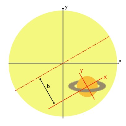
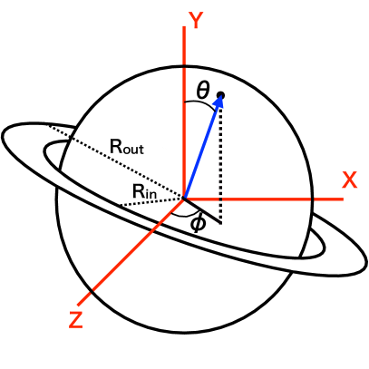
Figure 1: (Left) Schematic illustration of a transit of a planet with a ring. The origin of $(X,Y)$ is shifted from the center of the planet to that of the star. The radius of the star is $R_{\star}$, the radius of the planet is $R_{\rm p}$ and the impact parameter of the planet is $b$. The $z$-axis and the $Z$-axis are toward the observer. (Right) Enlarged view of the planet with the ring. $R_{\rm in}$ and $R_{\rm out}$ are the inner and outer radii of the ring respectively. The obliquity angle $\theta$ and azimuthal angle $\phi$ are defined with respect to $(X,Y,Z)$-coordinate.

We assume a thin uniform ring with a constant optical depth $\tau$ for the light from the direction normal to the ring plane. Thus the fraction of the background stellar light transmitted through the inclined ring is given by $\exp(-\tau(\sin\theta\cos\phi)^{-1})$, and we define the shading parameter $T$ as $1-\exp(-\tau(\sin\theta\cos\phi)^{-1})$. In our simple ring model, the value of $T$, instead of $\tau$, fully specifies the effective optical transparency of the ring.

In summary, our simple ring model is characterized by five parameters; four ($R_{\rm in},R_{\rm out},\theta,\phi$) specify the geometry of the ring, the other is a shading parameter $T$. Instead of $R_{\rm in}$ and $R_{\rm out}$, we use dimensionless parameters in fitting,:

$$r_{\rm in/p}\equiv\frac{R_{\rm in}}{R_{\rm p}},\qquad r_{\rm out/in}\equiv\frac{R_{\rm out}}{R_{\rm in}}.$$ (1)

2.2 Transit signal of a ringed planet

The stellar intensity profile $I(x,y)$ under the assumption of the quadratic limb darkening law is expressed in terms of two parameters $u_{1}$ and $u_{2}$:

$$\frac{I(x,y)}{I_{0}}=\left[1-u_{1}(1-\mu)-u_{2}(1-\mu)^{2}\right]\left(\text{ $\mu\equiv\sqrt{1-\cfrac{x^{2}+y^{2}}{R_{\star}^{2}}}$}\right),$$ (2)

where $I_{0}$ is the intensity at the center of the star. The physical conditions on the profile require the following complex constraints on $u_{1}$ and $u_{2}$:

$$u_{1}+u_{2}<1,\;u_{1}>0,\;u_{1}+2u_{2}>0.$$ (3)

In this paper, we adopt $q_{1}=(u_{1}+u_{2})^{2}$ and $q_{2}=u_{1}/(2(u_{1}+u_{2}))$ instead of ($u_{1}$, $u_{2}$) following Kipping (2013). Then, Equations (2) and (3) are rewritten as

$$\frac{I(x,y)}{I_{0}}=\left[1-2q_{2}\sqrt{q_{1}}(1-\mu)-\sqrt{q_{1}}(1-2q_{2})(1-\mu)^{2}\right],$$ (4)

$$\text{with}\;\;\;\;\;\;\;0<q_{1}<1,\;0<q_{2}<1.$$ (5)

In this parametrization, $q_{1}$ and $q_{2}$ vary independently between 0 and 1. This is useful in finding best-fit parameters (Kipping 2013). For reference, the Sun has $q_{1}=0.49$ and $q_{2}=0.34$ ($u_{1}=0.47$ and $u_{2}=0.23)$ (Cox 2000).

Let $D(x,y,t)$ be the blocked fraction of light coming from the location on the stellar disk $(x,y)$. Due to the motion of the planet during a transit, $D(x,y,t)$ is time-dependent and given as

$$D(x,y,t)=\begin{cases}1&:\text{if $(x,y)$ is within the planetary disk}\\ T&:\text{if $(x,y)$ is within the ring disk, but out of the planetary disk}\\ 0&:\text{otherwise}.\end{cases}$$ (6)

Then the normalized flux from the the system is given by

$$F(t)=1-\frac{\int_{\text{stellar disk}}\,I(x,y)D(x,y,t)dxdy}{I_{\rm all}},$$ (7)

where the second term indicates the fraction of light blocked by a transiting ringed planet, and the total flux is

$$I_{\rm all}=\int_{\text{stellar disk}}I(x,y)dxdy=\pi I_{0}R^{2}_{\star}\left[1-\frac{2\sqrt{q_{1}}q_{2}}{3}-\frac{\sqrt{q_{1}}(1-2q_{2})}{6}\right].$$ (8)

We develop a reliable numerical integration method that solves the boundary lines of $D(x,y,t)$ as described in Appendix A. Our method achieves the numerical error less than $10^{-7}$ in relative flux, and this is much smaller than a typical noise of the Kepler photometric data.

2.3 Effects that are neglected in our model

We briefly comment on three effects that we neglect in the analysis below; finite binning during exposure time, planetary precession, and forward-scattering of the ring. While all of them are negligible for the Saturnian ringed planet with a long period, they may become important in other situations.

For the precise comparison of our light-curve predictions against the Kepler long cadence, we may have to take account of the finite exposure time (29.4 min) properly. In fact, the binning effect is shown to bias the transit parameter estimate in the case of short-period planets (Kipping 2010). For long-period planets that we focus on here, however, the transit duration is sufficiently longer than the finite exposure time. Thus the binning effect is not important. In the case of the transit of Saturn in front of the Sun, for instance, the fractional difference of the relative flux is typically an order of $10^{-5}$ between models with and without the binning effect. This value is an order-of-magnitude smaller than the expected noise in the Kepler photometric data. Thus we can safely neglect the binning effect in the present analysis.

The precession of a planetary spin would generate observable seasonal effects on the transit shape of a ringed planet (Carter & Winn 2010; Heising et al. 2015). Since our current target systems are extracted from those with a single transit, however, we can ignore the effect; the period of the precession is proportional to the square of the orbital period, and thus the precession effect during a transit is entirely negligible. Nevertheless, we note here that this could be an interesting probe of the dynamics of short-period ringed planetary systems that exhibit multiple transits.

In the present analysis, we consider the effect of light-blocking alone due to the ring during its transit. In reality, forward scattering (diffraction by the ring particles) may increase the flux of the background light. Let us consider light from the star to the observer through the ring particle with diameter $d$. First, light is emitted from the disk of the star, and arrives at the ring particles. The angular radius of the star viewed from the ring particles is about $R_{\star}/a$, where $a$ is the semi-major axis of the orbit, and $R_{\star}$ is the stellar radius. Next, the light is diffracted by the ring particles, and the extent of the diffraction is described by the phase function (Barnes & Fortney 2004); the rough diffraction angle can be estimated from the first zero of the phase function $\theta\simeq 0.61\lambda/d$, where $\lambda$ is wavelength of light. In particular, the effect of the diffraction becomes significant when the viewing angle $R_{\star}/a$ is comparable to the diffraction angle. Let us define the critical particle size $d_{\rm crit}$ by equating $R_{\star}/a$ with $\theta=0.61\lambda/d$;

$$d_{\rm crit}=0.61\,\frac{a\lambda}{R_{\star}}=0.63\,\text{mm}\left(\frac{a/R_{\star}}{2060}\right)\left(\frac{\lambda}{500\text{nm}}\right).$$ (9)

Barnes & Fortney (2004) discussed the effect of diffraction using $d_{\rm crit}$. When $d\geq 10d_{\rm crit}$, the diffraction angle is small, and light just behind the ring particles is diffracted to the observer. In this case, the diffraction does not affect the direction of light, and we may express the extinction due to absorption with a single parameter $T$.

When $d\leq d_{\rm crit}/10$, the diffraction angle is large, and the ring particles diffract light to wider directions. Then, the amount of light that reaches the observer significantly decreases, and we may model the extinction in terms of $T$.

In both cases, $d\geq 10d_{\rm crit}$ and $d\leq d_{\rm crit}/10$, the extinction can be modeled with a single parameter $T$. In the case of Saturn with the typical particle diameter $d=1$ cm, for instance, $d_{\rm crit}\simeq 0.63$ mm from Equation (9) satisfies $d>10d_{\rm crit}$, so our model can be used to calculate the light curves of Saturn observed far from the Solar System.

We should note that when the typical size of particles satisfies $d_{\rm crit}/10\leq d\leq 10d_{\rm crit}$, the forward scattering induces the rise in the light curve before the ingress and after the egress, and this effect can become the key to identify the signatures of the rings out of other physical signals. Incorporating the diffraction into the model, however, requires intensive computation, and this is beyond the scope of this paper.

3 Classification

In what follows, we present our methodology to search for planetary rings in the real data. Figure 2 shows the flow chart of the analysis procedure and its application. Methods in each step of the chart are described along with the results of analysis in the following sections.

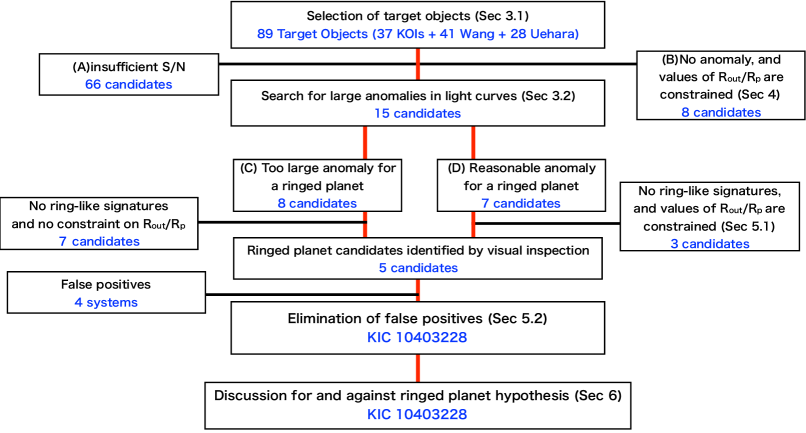
Figure 2: Flow chart of our strategy of ringed-planet search. Procedure and the number of remaining candidates are described in each step. The details of each procedure are described in the corresponding sections. For classification into (A)$\sim$(D), model I is adopted in Table 2.

In this section, we first choose target objects found in the Kepler field. Then, we classify them into four categories depending on the observed anomalies in the light curves. The details of classification procedure may be found in Appendices B and C.

3.1 Target Selection

The Kepler mission monitored more than 150,000 stars over four years, and identified about 8,000 planet candidates as Kepler Objects of Interest (KOIs). In this paper, we focus on long-period planet candidates because icy ring particles as observed around Saturn are supposed to survive only at locations far from the host star. Considering that the temperature of the snow line is $170$ K (Hayashi 1981), we choose 37 KOIs whose equilibrium temperatures are less than 200 K. In addition, we selected planet candidates reported by recent transit surveys; 41 candidates from a search by Wang et al. (2015) and 28 candidates from Uehara et al. (2016). In Table 1, the numbers of planetary candidates in three groups are listed with the number of transits.

We exclude several systems, which are not suited for our search. For KOI-5574.01 in KOIs and KIC 2158850 in Wang et al. (2015), we cannot find the transit signal among the noisy light curves. For KOI-959.01 in KOIs with $P=10$ days and KIC 8540376 in Wang et al. (2015) with $P=31.8$ days, we cannot neglect the binning effect due to the short transit duration. After removing these systems, 89 planet candidates are left in total for our search. Tables 1 summarizes the number of targets, and Figure 3 shows the overlapped objects among KOIs, Wang et al. (2015), and Uehara et al. (2016)

Table 1: Number of planet candidates in three groups.

Group	Number of systems			Total number of candidates
	One transit	Two transits	more than two transits
KOIs ($T_{\rm eq}\leq 200$ K)	5	2	30	37
Wang et al. (2015)	17	14	10	41
Uehara et al. (2016)	28	0	0	28

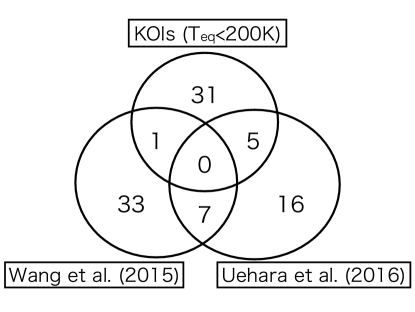
Figure 3: Venn diagram for target objects corresponding to Table 1.

3.2 Classification of target objects

Inevitably a signature of a possible ring around a planet is very tiny. Long-period planet candidates exhibit a small number of transits (Table 1), and the precision of the transit light curves is not improved so much by folding the multiple events. Therefore the search for a possible ring signature crucially relies on the quality of the few transiting light curves for individual systems.

According to the automated procedures described in Appendices B and C, we classify the long-period planet candidates into the following four categories.

(A) insufficient $S/N$ to constrain ring parameters:
  Since the anomalous feature due to the ring is very subtle, one cannot constrain the ring parameters at all if the intrinsic light-curve variation of the host is too large to be explained by any ring model. Thus we exclude those systems that exhibit a noisy light curve out-of-transit. The exclusion criteria depend on the adopted ring model to some extent, but are determined largely by the threshold signal-to-noise ratio $(S/N)$ that we set as $S/N=10$. For definiteness, we consider 4 different ring models (Table 2), and the details of the procedure are described in Appendices B and C.

(B) sufficient $S/N$ and no significant anomaly:
   A fraction of the systems has a sufficiently good $S/N$ and exhibits no significant anomaly. In such a case, we can put physically meaningful constraints on the possible ring parameters (Section 4).

(C) too large anomaly for a ringed planet:
  In contrast to (B), some systems exhibit a large anomaly in the transiting light curve that exceeds the prediction in the adopted ring models. Nevertheless, different ring models may be able to explain the anomaly, and we still continue to search for ringed planets in this category (Section 5).

(D) reasonable anomaly for a ringed planet
  Finally a small number of systems with a good $S/N$ indeed exhibit a possible signature that could be explained by the ring model. We perform additional analysis to test the validity of the ring hypothesis in a more quantitative fashion (Section 5 and 6).

The above classification is done on the basis of observed anomalies, which are derived by fitting a planet model to light curves. The data are taken form the Mikulski Archive for Space Telescopes (MAST), and we use the Simple Aperture Photometry (SAP) data taken in the long-cadence mode (29.4 min). In fitting, we use only the first transit in the light curve for each candidate in deriving the observed anomaly for simplicity. After fitting the planet model to data, the long-period planet candidates are automatically classified into the above categories (A)$\sim$(D). Table 2 summarizes the results of classification for four models. In a later section, we use the classification according to model I, which contains more candidates in categories (B)$\sim$(D) than the other three. In fact, the choice of model I is partly reasonable because the distant planets potentially have tilted rings like Saturn because of low tidal force.

As candidates in (A) have insufficient $S/N$ for further analysis, we do not consider them in the following analysis. In section 4, we obtain upper limits on $R_{\rm out}/R_{\rm p}$ for candidates in (B). In section 5, we first search for the ringed planets in categories (C) and (D) by visual inspection, and later examine the reliability of transits more quantitatively. In section 6, we interpret the possible ringed planet candidate.

Table 2: Parameters and classification.

Parameters	Meaning
$P$(day)	Period	$10759$
$a/R_{\star}$	Scaled semi-major axis	$2059.67$
$q_{1}$	Limb darkening parameter	$0.49$
$q_{2}$	Limb darkening parameter	$0.34$
$t_{0}$(day)	Time of a transit center of a planet	$0$
$T$	Shading coefficient	$1.0$
$r_{\rm in/p}$	Ratio of $R_{\rm in}$ to $R_{\rm p}$	$1.0$
$r_{\rm out/in}$	Ratio of $R_{\rm out}$ to $R_{\rm in}$	$\cdots$
$R_{\rm p}/R_{\star}$	Planet to star radius ratio	$\cdots$
		model I (Fiducial)	model II	model III	model IV
$b$	Impact parameter	0.8	0.5	0.8	0.5
$\theta$(deg)	Angle between $Y$-axis and axis of the ring	45	45	$\arcsin(0.1)$	$\arcsin(0.1)$
$\phi$(deg)	Angle between $Z$-axis and	45	45	0	0
	ring-axis projected onto $(Z,X)$-plane
$r_{\rm eq}$	Boundary value, above which the sky-projected	2.0	2.0	10.0	10.0
	ring is larger than the planetary disk
	(see Section B.3 for detailed explanation)
	Classification	Number of classified systems
	(A) insufficient $S/N$	66	82	80	82
	(B) sufficient S/N to $R_{\rm out}/R_{\rm p}$	8	1	2	1
	(C) too strong anomaly	8	3	4	4
	(D) possible candidate	7	3	3	2

4 Upper limits of $R_{\rm out}/R_{\rm p}$ for candidates in (B)

Upper limits on $R_{\rm out}/R_{\rm p}$ are given for candidates in (B) as a result of classification. Figure 4 shows the light curves and fitted curves of eight candidates classified to (B) in model I. They show no appreciable anomalies in the residual relative to the single planet model. For these candidates, we could detect the ring signature if exists. Thus in turn, we can derive the upper limits on $R_{\rm out}/R_{\rm p}$. This is done by simply comparing the expected anomaly in model I and the observed anomaly in the light curve. The details of the method to place upper limits on $R_{\rm out}/R_{\rm p}$ are described in Appendix B and C, and the results are summarized in Table 3.

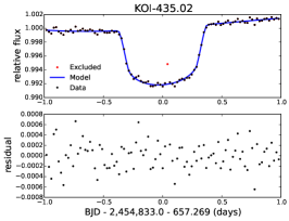
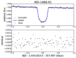
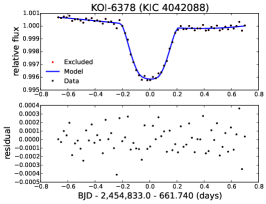
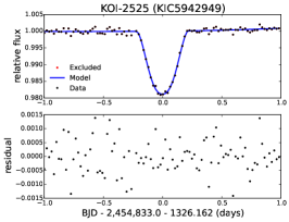
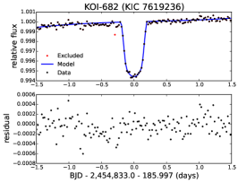
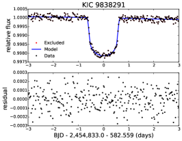
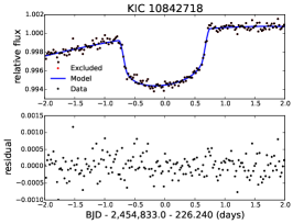
Figure 4: Candidates in (B) with sufficient $S/N$ to constrain $R_{\rm out}/R_{\rm p}$. The light curves (black circles) are shown with the best-fit planet models (blue lines). The red points are excluded in fitting. The horizontal axis shows time in BKJD = BJD - 2454833.0 (the Barycentric Kepler Julian Date) offset by the central time of the transit.

Table 3: Upper limits of radii of outer rings.

Name	Upper limits of $R_{\rm out}/R_{\rm p}$ in model I	$R_{\rm p}(R_{J})$	$a$(AU)	Transit Epoch (BKJD)
Candidates in (B)
KOI-435.02	1.5	0.66	1.28	657.269
KOI-1466.01	1.5	1.13	1.14	357.997
KIC 4042088	1.2	2.94	0.78	617.65
KIC 4042088	1.95	0.85	1.41	661.74
KIC 5942949	1.5	1.18	1.13	1326.162
KIC 7619236	1.7	0.71	1.35	185.997
KIC 9838291	1.9	0.42	14.3	582.559
KIC 10842718	1.6	0.75	7.60	226.300
Candidates in (D)
KOI-490.02	1.2	1.16	2.53	492.772
KOI-868.01	1.2	0.76	0.74	208.401
KIC 8012732	1.8	0.67	0.68	391.807
KIC 8410697	1.8	0.77	3.19	542.122

5 Search for ringed planets

In this section, we search for ringed planets in categories (C) and (D), extract the tentative ringed planet candidates, and examine whether the transits are not false positive.

5.1 Tentative selection of possible ringed planets

Figures 5 and 6 show the light curves of candidates in categories (C) and (D), respectively. Candidates in (C), where the observed anomaly exceeds the prediction of model I, may be consistent with other ringed planets in different configurations. Thus, we search for ringed planets not only in (D) but also (C).

We extract ringed planet candidates by visual inspection of their light curves on the basis of following properties expected for ringed planets:

• Duration of ingress and/or egress is long.

• Transit shape is asymmetric due to the non-zero $\phi$.

As a result, we identify five systems KOI-771(D), KOI-1032(C), KOI-1192(D), KOI-3145(D), and KIC 10403228(D) as tentative ringed planets. For the other four candidates in (D), which show no visible ring-like feature in the light curves, we obtain the upper limits on $R_{\rm out}/R_{\rm p}$ in the same method as in the previous section (Table 3). In total, we obtain the upper limits on $R_{\rm out}/R_{\rm p}$ for 12 candidates, and the six of them have $R_{\rm out}/R_{\rm p}\leq 1.5$.

For six candidates in (C) with no ring-like features, we cannot set the upper limits of ring parameters, and we conclude that the signals are not due to rings, but are due to the temporal stellar activities.

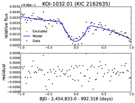
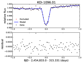
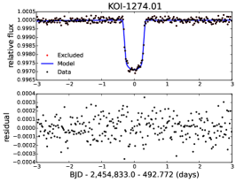
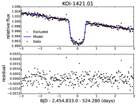
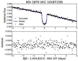
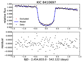
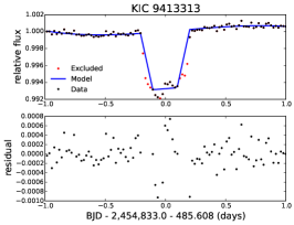
Figure 5: Candidates in (C) with too large anomaly for a ringed planet. The format of the figure is the same as Figure 4.

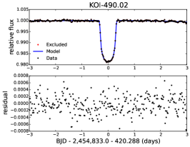
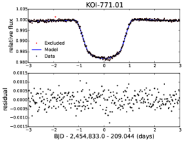
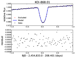
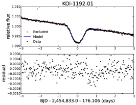
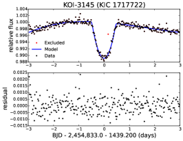
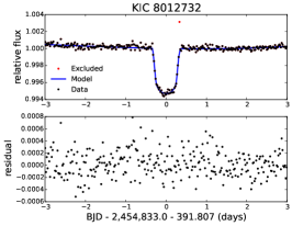
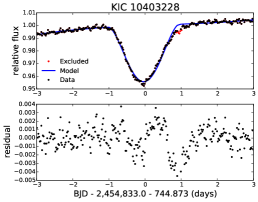
Figure 6: Candidates in (D) with moderate anomaly for a ringed planet. The format of the figure is the same as Figure 4.

5.2 Elimination of false positives

We examine the reliability of transit signals for the five preliminary candidates. As a result, we find that four are false positives, and KIC 10403228 still passes all criteria. More specifically, we regard a target as a false positive if one of the following criteria is satisfied (Coughlin et al. 2016).

1. The target object exhibits a significant secondary eclipse, which is expected for an eclipsing binary.

2. None of our candidates exhibits the secondary eclipse.

3. The signal originates from the other nearby stars or instrumental noise.

4. Inspecting Target Pixel Files, we found that the dips in the light curves of KOI-1032.01, KOI-1192.01, and KOI-3145 do not come from the target stars. Figure 7 shows an example of KOI-1192.01. Community Follow-up Observing Program (CFOP) classifies KOI-1032.01 as a false positive (Uehara et al. 2016). Wang et al. (2015) and Uehara et al. (2016) also indicate that KOI-1192.01 and KOI-3145 are false positivities. Moreover, we find that the transit depths in the light curves of KOI 771.01 differ in many pixels, and the contaminations from the non-target stars are very strong. Wang et al. (2015) also pointed out that this system is false positive. For KIC 10403228, the transit depths differ in only two pixels, while it is constant in the other pixels, so we conclude that the signal is originated from the target star. The more detailed discussion of KIC 10403228 is presented in a later section.

5. The transit simultaneously occurs at different stars in different pixels. This indicates that the signal does not originate from the target but from the instrumental noise.

6. The transit events of KOI-1032.01 and KOI-1192.01 are located at the same time. This result is consistent with that of the Criterion 2.

7. The shape of the light curve is inconsistent with that of a transiting object.

8. From Figures 5 and 6, all signals fit well to transit-like features.

KIC 10403228 is the single system that passes all the criteria. Thus, we move on to the detailed pixel-based analysis next.

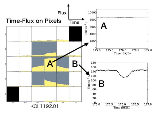
Figure 7: Indication that KOI-1192.01 is a false positive. The light curves of the pixels labeled as A and B are shown in the right panels. The pixel located at A receives the largest amount of light among pixels of the target star, and the pixel located at B receives the small amount of light. The very different relative depths in the two pixels indicate that the signal does not originate from the target star at the center.

5.3 Detailed pixel analysis on KIC 10403228

KIC 10403228 is considered to be an M dwarf and has a nearby star separated by about 3 arcsec (Rappaport et al. 2014). According to the data taken by United Kingdom Infrared Telescope (UKIRT), the nearby star is located at (RA, Dec) = $(19^{\rm h}\,24^{\rm m}\,54.25^{\rm s},\;+47^{\circ}\,32^{\prime}\,57.5^{\prime\prime})$ and its J-band flux is about $1/5$ of KIC 10403228. Here we examine the possibility that the transit is associated with this nearby star rather than KIC 10403228.

Figure 8 shows the light curve and fractional depth of the transit event in each of the pixels around KIC 10403228. The small transit depths in pixels A and B suggest that the source of the transit is not the nearby star shown by a red filled star, because otherwise the transit depths should be larger in those pixels close to the nearby star. To confirm this fact in a more quantitative way, we also calculate the centroid offset using the pixel-level light curves. As a result, we find that the flux centroid moves towards the nearby star during the transit and that the displacement is comparable to the value expected from the observed transit depth ($5\%$) and the flux ratio in J-band ($5:1$). The variation of the transit depth and the centroid displacement consistently indicate that the transit is not due to the nearby star. While we may be able to evaluate the contamination on the light curve from this nearby star more quantitatively, it does not change our conclusion in any case, and we do not perform the detailed analysis for simplicity.

We note that the transit signal contains a clear short-period modulation (panel B in Figure 8). Since the modulation is not visible at panel C, it is most likely due to the nearby star. Actually, there is another long-period modulation with $P\simeq 35$ days in the light curve, which may come from the target star. If these periods are related to the stellar spins, the nearby star is a fast rotating star, and the target star is a slow rotator. Thus, we may ignore the effect of gravity darkening of the target star.

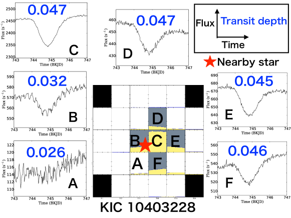
Figure 8: Light curves on pixels are shown along with the approximate depth of the transit. A red star expresses the position of the nearby star. The depth is shallow in the left side of the region, where the contamination from the nearby star is large.

6 Detailed analysis of a possible ringed planet KIC 10403228

For the further study of KIC 10403228, we present and discuss three possible models accounting for the data: “planetary ring scenario”, “circumstellar disk scenario”, and “hierarchical triple scenario”. We also discuss other possibilities than the above three models.

6.1 Interpretation with a ringed planet

We fit various models with and without the ring to the light curve of KIC 10403228 by minimizing the value of $\chi^{2}$ defined in Equation (B4). In practice, we use $\pm 3.09$ days-time window to trim 300 data points centered around $T_{0}=744.773$ day (BKJD [= BJD$-2454833$ day]). To remove the long-term flux variations in the light curve, we adopt the model in Equation (B5) that is composed of a fourth-order polynomial and the transit model $F(t)$ in Equation (7). The standard deviation $\sigma$ is estimated to be $9.17\times 10^{-4}$ from the out-of-transit data. This value is about 1.3 times larger than the error recorded in the SAP data.

As the transit of KIC 10403228 is observed just once, we cannot infer the orbital period from the timing of the transit. However, we can infer it from Kepler’s law. The depth and V-shape of the observed transit imply that the transiting object is relatively large and grazing. Thus, we approximate the total transit duration $T_{\rm tra}$ as

$$T_{\rm tra}\simeq P\left(\frac{2R_{\star}}{2\pi a}\right)\left(\frac{\sqrt{1-e^{2}}}{1+e\sin\omega}\right),$$ (10)

where the last factor is a correction term due to an eccentricity $e$ with $\omega$ being the argument of periapse. From Kepler’s law and Eq (10), one obtains

$$P\simeq 450\text{ years}\left(\frac{\rho_{\star}}{\text{ 12.6 g cm}^{-3}}\right)\left(\frac{T_{\rm tra}}{\text{2 days}}\right)^{3}\left(\frac{1+e\sin\omega}{\sqrt{1-e^{2}}}\right)^{3}.$$ (11)

We obtain $P\simeq 450$ years if we adopt $e=0$ and $T_{\rm tra}=2$ days for the transit duration of KIC 10403228, and the stellar density $\rho_{\star}=12.6\pm 6.0$ g cm^-3 from Wang et al. (2015). The stellar density in Wang et al. (2015) is adopted from Dressing & Charbonneau (2013), who estimated the stellar properties by comparing the observed colors taken in 2MASS and SDSS with the Dartmouth model (Dotter et al. 2008).

Before fitting, we simply examine how often we expect to see a transit of a planet with $P\simeq 450$ years. Assuming that all the stars host planets with $P\simeq 450$ years, the expected number of transit detections is given by

$$n_{\rm tra}=0.045\left(\frac{N_{\rm target}}{150,000}\right)\left(\frac{t_{\rm obs,dur}/P}{4\text{ years}/450\text{ years}}\right)\left(\frac{R_{\star}/a}{1/25,000}\right),$$ (12)

where $a/R_{\star}=25000$ is the fiducial value estimated from equation (10), $t_{\rm obs,dur}$ is a observational period, and $N_{\rm target}$ is the number of target stars. The adopted values of $t_{\rm obs,dur}$ and $N_{\rm target}$ are the typical values of Kepler. The frequency of planets with $P=450$ yrs would be less than 1, so we may see $n_{\rm tra}$ as the optimistic upper limit of the expected value. This current value of $n_{\rm tra}=0.045$ is small, but not too unlikely. Apart from the tiny ring-like feature, the overall shape of the signal is clearly due to the transiting event, and it is very difficult to explain the feature from the stellar activities.

We would like to comment on the reliability of $P\simeq 450$ years. The key parameters are $\rho_{\star}$ and the eccentricity in Eq (11). For example, if the system is a giant star rather than an M dwarf, the density and the period become smaller. In this sense, to specify the correct stellar density, we would need a follow-up observation. Moreover, the eccentricity can also change the estimated period in Eq (11). If $e=0.6$, the period can be changed by the factor of $(1/8.0)$–$8.0$, and if $e=0.9$, the factor of change is within $(1/82.82)$–$82.82$ (or 5 years $<P<$ 34,000 years). Thus, the planet with a relatively short period and a large eccentricity can also explain the data. Although the period is uncertain, the different period does not change the fitting results, so we adopt $P=450$ years for the fiducial value for the time being.

For fitting, we adopt $P=450$ years, and $q_{1}$ and $q_{2}$ from the official catalog of Kepler. In summary, there are nine free parameters, $t_{0},R_{\rm p}/R_{\star},b,a/R_{\star}$, and $c_{i}$ ($i=$0–4) for the model without the ring, and five additional parameters $\theta,\phi,r_{\rm in/p},r_{\rm out/in}$ and $T$ for the model with ring. We set the initial values of $c_{i}$ ($i=$0–4) to those obtained from a polynomial curve fitting for the out-of-transit data.

First, we fit the planet alone model to the data. The blue line in Figure 9 is the best-fit model without the ring. The best-fit parameters are listed in Table 4. The residuals from the fit clearly have some systematic features, and the planet alone model fails to fully explain the light curve, in particular, around 745.8 day (BKJD) in Figure 9. Therefore, we attempt to interpret the data with the ringed planet model. After trying a lot of initial values for fitting, we finally find two solutions, which give at least local minima of $\chi^{2}$ in Equation (B4). Figure 9 shows those two solutions in the red and green lines. The best-fit parameters are shown in Table 4. The geometrical configurations for both solutions are shown in Figure 10. Clearly, models with the ring significantly improve the fit.

In Table 4, values of $R_{\rm p}$, $R_{\rm in}$, and $R_{\rm out}$ are calculated on the assumption of $R_{\star}=0.33\pm 0.05\,R_{\odot}$ (Wang et al. 2015). It turns out that the resulting ratio of ring and planet radii is similar to that of Saturn: $R_{\rm in}\simeq 1.5R_{\rm p}$ and $R_{\rm out}\simeq 2.0R_{\rm p}$.

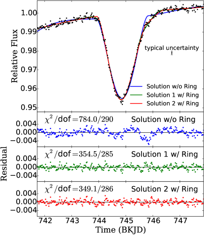
Figure 9: Comparison of the light curve of KIC 10403228 (black data) with the models with ring (red line & green line) and without ring (blue line). We found different configurations for the model with ring. While the model without ring cannot explain the data around 745.8 day (BKJD), the ringed planet model fits the data well. Residuals and $\chi^{2}$ of fit are shown in each panel.

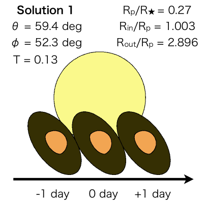
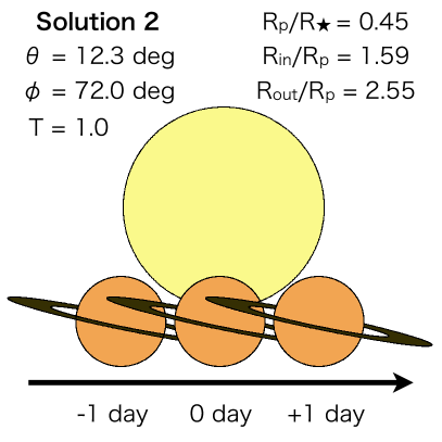
Figure 10: Schematic illustration of the ringed planet models for the two best-fit solutions. Positions of the planet are shown at $-1,0,+1$ day from the central time of the transit of the planet. Note that the occultation of the star due to the ring continues even after the transit of the planet is completed.

Table 4: Best fit parameters for the transit of KIC 10403228

	Single planet	Ringed planet (solution 1)	Ringed planet (solution 2)
Fixed parameters
$P$ (years)	$450$	$450$	$450$
$q_{1}$	$0.6737$	$0.6737$	$0.6737$
$q_{2}$	$0.0767$	$0.0767$	$0.0767$
Variables
$t_{0}$ (day)	$0.065\pm 0.0021$	$0.017\pm 0.016$	$0.0386\pm 0.0052$
$R_{p}/R_{\star}$	$0.46\pm 9.09$	$0.27\pm 0.33$	$0.45\pm 0.05$
$b(=a\cos i/R_{\star})$	$1.16\pm 10.6$	$0.99\pm 0.44$	$1.14\pm 0.06$
$a/R_{\star}$	$24275.0\pm 31617.1$	$25394.5\pm 765.0$	$25743.9\pm 215.6$
$T$	$\cdots$	$0.13\pm 0.07$	$1.0$ (converged to upper bound)
$\theta$(deg)	$\cdots$	$59.4\pm 45.0$	$12.3\pm 4.0$
$\phi$(deg)	$\cdots$	$52.3\pm 24.9$	$72.0\pm 4.5$
$R_{in}/R_{p}$	$\cdots$	$1.003\pm 2.95$	$1.59\pm 0.42$
$R_{out}/R_{in}$	$\cdots$	$2.89\pm 8.0$	$1.61\pm 0.59$
$c_{0}$	$0.9972\pm 0.0002$	$1.00023\pm 0.00034$	$0.9999\pm 0.0003$
$c_{1}$	$0.00066\pm 0.00008$	$0.0014\pm 0.0001$	$0.0015\pm 0.0001$
$c_{2}$	$0.00067\pm 0.00011$	$-0.00047\pm 0.00015$	$-0.00030\pm 0.00013$
$c_{3}$	$0.000158\pm 0.000013$	$0.000053\pm 0.000015$	$0.000038\pm 0.000015$
$c_{4}$	$-0.000072\pm 0.000011$	$0.000021\pm 0.000014$	$0.000005\pm 0.000012$
(Given $R_{\star}=0.33\pm 0.05\,R_{\odot}$)
$R_{\rm p}\,\,(R_{J}\,\,^{a})$	$1.48\,\,^{b}\,$	$0.88\pm 1.07$	$1.44\pm 0.27$
$R_{\rm in}\,\,(R_{J}\,\,^{a})$	$\cdots$	$0.89\pm 2.65$	$2.29\pm 0.72$
$R_{\rm out}\,\,(R_{J}\,\,^{a})$	$\cdots$	$2.56\pm 1.36$	$3.69\pm 0.23$
(Statistical values)
$\chi_{\rm red}^{2}$ (=$\chi^{2}$/dof)	$2.70$ (=$784.0$/290)	1.24 (=354.5/285)	1.23 (=$349.1/286\,\,^{c}$)

We comment on the implication of the fitted model for KIC 10403228 in the following. The radiative equilibrium temperature of the ring particle is given by

$$\;\;\;\;\;\;\;\;T_{\rm eq}\simeq 15.1\,\text{K}\left(\frac{25000}{a/R_{\star}}\right)^{0.5}\left(\frac{T_{\star}}{3386\,\text{K}}\right)\left(\frac{1-A}{1-0.5}\right)^{0.25},$$ (13)

where we fiducially adopt the Bond albedo of the ring particle $A$ of 0.5. The stellar effective temperature $T_{\star}=3386$ K of KIC 10403228 is taken from Wang et al. (2015). Since the equilibrium temperature expected from the model is much lower than the temperature $170$ K at the snow line (Hayashi 1981), icy particles around the planet can survive against the radiation of the host star.

The best-fit values of $\theta=59.4^{\circ}$ for solution 1 implies a significantly tilted ring with respect to the orbital plane, and $\theta=12.3^{\circ}$ for solution 2 implies a slightly tilted ring. We examine the stability of those tilted rings on the basis of a simple tidal theory. Under the assumption that the ring axis is aligned with the planetary spin, the damping timescale of the ring axis is equal to that for the orbital and equatorial planes of the planet to be coplanar. This time-scale is given by a tidal theory (e.g. Santos et al. 2015):

$$\;\;\;\;\;\;\;\;\;\;\;\tau_{\rm tidal} =\frac{P_{\rm orb}Q}{9\pi k_{2}}\frac{\rho_{p}}{\rho_{s}}\left(\frac{a}{R_{\star}}\right)^{3}\simeq\frac{GP_{\rm orb}^{3}Q}{27\pi^{2}k_{2}}\rho_{p}$$

$$=6.94\times 10^{16}\,\text{yr}\left(\frac{P_{\rm orb}}{450\,\text{years}}\right)^{3}\left(\frac{2.3\times 10^{-4}}{k_{2}/Q}\right)\left(\frac{\rho_{p}}{0.70\,\text{ g\,cm${}^{-3}$ }}\right),$$ (14)

where $P_{\rm orb}$ is an orbital period, $Q$ is a dissipation factor, and $k_{2}$ is the second Love number. If we adopt $k_{2}/Q=2.3\times 10^{-4}$ (Lainey et al. 2012) and $\rho_{p}=0.70$ gcm^-3 (Cox 2000) of Saturn, the damping timescale is sufficiently long. Thus, the best-fit configurations are consistent with the spin damping theory even under the assumption that the equatorial plane of the planet is coplanar with the ring plane. Thus, the tilted rings of our best-fits also imply the non-vanishing obliquity of the planet.

The ringed planet model is consistent with the data. However, the V-shape of the transit (Figure 9) is also a typical feature of eclipsing binaries, and the estimated period $\sim 450$ yrs may be too long to be detected in four years of Kepler’s observation (Equation (12)). Therefore, we discuss other scenarios without a planetary ring. For this purpose, in the following, we present two possible hypotheses, which can also explain the data; a binary with a circumstellar disk and a hierarchical triple.

6.2 Interpretation with a circumstellar disk

In this section, we pursue the possibility that the current transit is caused by an eclipsing-binary with a circumstellar disk rather than a planetary ring. Actually, the fitting result in the previous section is also applicable to this binary scenario, so we may compare the plausibilities of the eclipsing-binary and planet scenarios to test the circumstellar disk model. For this specific purpose, we use the public code VESPA (Validation of Exoplanet Signals using a Probabilistic Algorithm) (Morton 2012, 2015). With VESPA, we compare the likelihoods of the following four scenarios; “HEBs (Hierarchical Eclipsing Binaries)”, “EBs (Eclipsing Binaries)”, “BEBs (Background Eclipsing Binaries)”, and “Planets” (Transiting Planets) adopting a variety of different periods.

We adopt $JHK$-magnitudes from 2MASS ($\text{J-mag}=13.429\pm 0.028$, $\text{H-mag}=12.793\pm 0.03$, and $\text{K-mag}=12.518\pm 0.027$), (RA, Dec) = $(19^{\rm h}\,24^{\rm m}\,54.413^{\rm s},\;+47^{\circ}\,32^{\prime}\,57.5^{\prime\prime})$, maxrad = 3.0 arcsec (angular radius of the simulated region), $\text{Kepmag}=16.064$, and $R_{\rm p}/R_{\star}=0.3$. In reality, those observed colors might be contaminated by the nearby star discussed in Section 5.3, but we assume that the contamination is sufficiently small in the present analysis. Given these inputs, VESPA calculates the star populations and the probability distribution of transit shape parameters for the above four scenarios. For our adopted set of input parameters, VESPA identifies the primary star as an M dwarf consistent with the classification of Dressing & Charbonneau (2013). We repeat the simulation ten times with different initial random numbers according to the prescription of VESPA.

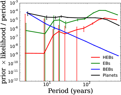
Figure 11: Relative probability of different models against adopted periods. The values in the vertical axis include the prior and likelihood factors, and the observational probability. Each point is slightly offset for visibility.

Figure 11 shows the relative probability of each scenario for different assumed periods. We define the relative probability as the product of the “prior” and “likelihood” computed by VESPA, multiplied by $1000\,\mathrm{days}/P$. The last factor $1000\text{ days}/P$ corrects for the probability that a long-period transit is observed in a given observing duration much shorter than the orbital period, which is not taken into account in the “prior” of VESPA. The plot shows the medians and the standard deviations of the probabilities computed from 10 sets of simulations. While the binary scenarios are more likely than the Planets scenario for the shortest and the longest periods investigated here, the Planets scenario is the most preferred in the intermediate region (10 years $\lesssim P\lesssim$ 100 years). The result suggests that the planetary interpretation of the light curve is not so unlikely compared to the binary scenario, although there is a fair amount of probability that this is a false positive. Another important implication of Figure 11 is that the likelihood of orbital periods in the Planets scenario is much broader than what we intuitively thought before, and not sharply peaked around 450 years.

While Figure 11 represents our final result from VESPA, we point out two additional factors that may be of importance for more detailed arguments.

First, the period distribution and the overall fraction of long-period planets and binaries have not been taken into account. Occurrence rate of giant planets around M dwarfs is given by Clanton & Gaudi (2016). They estimated the frequency of the planets with $10^{2}M_{\oplus}<M_{\rm p}<10^{3}M_{\oplus}$ to be $0.039^{+0.042}_{-0.025}$ for $10^{3}\text{ days}<P<10^{4}\text{ days}$ and $0.013^{+0.025}_{-0.010}$ for $10^{4}\text{ days}<P<10^{5}\text{ days}$. On the other hand, Janson et al. (2012) estimated the multiplicity distribution of the binaries in $3$–$227$ AU and found the overall occurrence rate $0.27\pm 0.03$ peaked around 10 AU. These results imply that planets around M dwarfs is rarer than its stellar companion by one or two orders of magnitude. This difference in the overall frequency may further increase the relative plausibility of the EBs scenario compared to the Planets scenario.

Second, what also matters in reality is the frequency of planetary rings and circumstellar disks that produce the observed anomaly in addition to the transit signal. It is, however, far beyond our current knowledge to estimate these factors rigorously.

Given these difficulties, follow-up spectroscopy or high-resolution imaging would be more feasible to distinguish the EBs and Planets scenarios.

6.3 Interpretation with a hierarchical triple

An eclipse due to a close binary (rather than a single star/planet) on a wide orbit around the primary M star is yet another possibility to explain the asymmetric and long transit-like signal observed for KIC 10403228. This is because the orbital motion of the occulting binary can produce the acceleration that modifies the in-eclipse velocity of the occulting object(s) relative to the primary. To test this possibility, we consider a hierarchical triple system consisting of a short-period binary (“inner” binary) orbiting around and eclipsing the primary M star on a wide orbit (“outer” binary). In the following, we only take into account the luminosity of the occulted star and ignore the flux from the smaller binary. We also assume the orbits of both inner and outer binaries are Keplerian, and use the subscripts “in” and “out” to denote their parameters. A mass ratio of the inner binary is fixed to 1 for simplicity. In this model, the motion of the two components of the inner binary is specified by $t_{\rm 0,in}$ (inferior conjunction of the inner binary), $P_{\rm in}$, $a_{\rm out}/a_{\rm in}$, $i_{\rm in}$, $\Omega_{\rm in}$ (longitude of ascending node relative to that of the outer binary), in addition to the parameters for a single-planet model (now with the subscripts “out”). We fit all of these parameters except that the stellar density $\rho_{\star}=13.0\text{gcm}^{-3}$, $q_{1}=0.6737$, $q_{2}=0.767$, the time offset $T_{\rm 0}=744.773$ days in Eq (B5), and the same baseline as obtained in Table 4 (solution 2) are fixed. The mass ratio of the outer binary is related to $P_{\rm in}$, $P_{\rm out}$, and $a_{\rm out}/a_{\rm in}$ as

$$q\equiv\frac{M_{\rm in}}{M_{\rm out}}=\frac{1}{(a_{\rm out}/a_{\rm in})^{3}(P_{\rm in}/P_{\rm out})^{2}-1},$$ (15)

where $M_{\rm in}$ is a total mass of the inner binary, and $M_{\rm out}$ is the mass of the primary star.

Figure 12 shows one of the best-fitting models with $P_{\rm out}=1396.615$ days, $a_{\rm out}/a_{\rm in}=54.53$, $\Omega_{\rm in}=-0.00945$, $P_{\rm out}=10.96$ days, $b_{\rm out}=2.024$, $\cos i_{2}=0.103$, $t_{\rm 0,out}=1.965\times 10^{-3}$ days, and $t_{\rm 0,in}=1.965\times 10^{-5}$ days. In this solution, we find $q=0.0956$, which leads to $M_{\rm in}=30M_{\rm J}$. We also obtain $\chi^{2}/\text{dof}=379.3/292$, which is comparable to the ringed-planet model. In this solution, the observed $\sim 2\,\mathrm{days}$ duration is reproduced despite that the value of $P_{\rm out}$ is much shorter than required for the planetary scenario. This is made possible because the orbital motion of the inner binary cancels out the high orbital velocity of the outer binary. In addition to this particular solution, we find various other solutions with similar $\chi^{2}$ values for a wide range of $P_{\rm out}$. In general, the solutions with longer $P_{\rm out}$ are found to correspond to smaller $q$; for example, we find $q\simeq 0.02$ for $P_{\rm out}\simeq 30\text{\,yrs}$, and $q\simeq 0.003$ for $P_{\rm out}=300\text{\,yrs}$. For $M_{\star}=0.3M_{\odot}$, these mass ratios $q=(0.1,0.02,0.003)$ translate into $M_{\rm in}=(30M_{\rm J},6M_{\rm J},M_{\rm J})$. Thus, in this scenario, the system can be composed of three low-mass stars or a star with a binary planet.

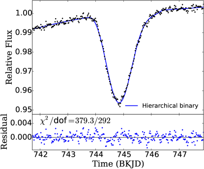
Figure 12: Light curve of KIC 10403229 and fitting curve with a model of a hierarchical triple.

The advantage of this scenario is that the observed long transit can be reproduced with much smaller $P_{\rm out}$ than in the ringed-planet model, which leads to far higher transit/eclipse probability. On the other hand, it is also true that the parameters need to be finely tuned to cancel the two orbital motions. While the degree of required fine tuning is crucial in comparing the evidence of this hypothesis with the planetary or stellar ring models, the evaluation of this factor is not trivial given the large parameter space. In addition, there still remain uncertainties in frequency of the hypothetical hierarchical triple (three low-mass stars or a star with a binary planet). Given these complexities, it is difficult to conclude whether or not this scenario is favored compared to the above two. Again, the follow-up observation will be effective for the further study.

6.4 Possibilities other than a ringed object and a hierarchical triple

So far, we present the three leading scenarios “planetary ring scenario”, “circumstellar disk scenario”, and “hierarchical triple scenario”. There still remain other possibilities that may potentially account for the light curve of KIC 10403228. In this section, we examine these possibilities and show that they are unlikely to explain the data. Throughout this section, we basically assume that the transit is caused by a planet, but the results in this section are also applicable for the stellar eclipse.

6.4.1 Oblate planet

A significant oblateness of a single planet may mimic a ring-like anomaly during a transit. Indeed our model reduces to an oblate planet if we set $R_{\rm p}=0$, $R_{\rm in}=0$, and $T=1.0$ with an appropriate choice of $\theta$ and $\phi$. We attempt the fit of this oblate planet model to the light curve, and obtain the best-fit with $\chi^{2}/{\rm dof}=492.4/288$. This value is much larger than the best-fit value $\chi^{2}/{\rm dof}=349.1/286$ with the model with a ring. Furthermore, the best-fit oblate planet model requires the projected ellipticity of $f=(a-b)/a=0.79$, where $a$ is the major axis, and $b$ is the minor axis. This solution is an unstable configuration; the rotating object will break up due to the centrifugal force when $a\geq 1.5b$ (Equation (2.14) in Maeder (2009)). Thus, we conclude that the oblateness of the planet is unlikely to explain the observed anomaly.

6.4.2 Additional transit due to exomoon

In Section 6.3, we only consider an additional motion of an occulting object due to an accompanying object. However, a transit of the accompanying object (e.g. exomoon) itself is yet another possibility for the peculiar light curve of KIC 10043228. As shown below, this possibility is ruled out by the shape of the anomaly.

As shown in Figure 9, the anomaly in the light curve is significant only in the latter half. Motivated by this fact, we fit the light curve using the planet-alone model, masking the latter half of the transit and adopting the same baseline as obtained in Table 4 (solution 2); the difference between this model and the observed light curve would represent the anomalous contributions from anything other than the main transiting planet. The result in Figure 13 clearly shows that the anomaly consists of a short rise in the flux followed by a more significant dip. Such a feature is clearly inconsistent with the transit of an exomoon.

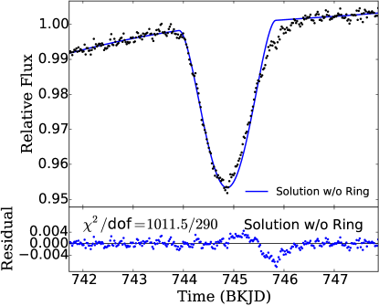
Figure 13: Planet-alone fit to only the first half of the transit light curve. The baseline polynomial is the same as that in solution 1 in Table 4. The anomaly consists of a rise followed by a dip.

6.4.3 Anomalies specific to in-transit data

There exist anomalies specific to in-transit data; spot crossing and gravity darkening. If the planet crosses spots on the stellar surface, the light curve is deformed (e.g. Sanchis-Ojeda et al. 2011). In general, however, spots are dark, so spot-crossing causes a bump in the light curve. The observed anomaly in the bottom panel of Figure 13 is inconsistent with a single bump, so the spot is unlikely to cause the anomaly. Gravity darkening makes the light curve asymmetric (e.g. Barnes et al. 2011; Masuda 2015). In section 5.3, we identify the target star as the slow-rotating star, and the gravity darkening is negligible. In conclusion, these mechanisms are unlikely to explain the ring-like signal in the light curve.

6.4.4 Stellar noise

The ring-like structure in the light curve shows up only for a short duration. Thus, the short-term stellar noise might mimic the ring-like anomaly just by chance. To discuss this possibility, we investigate the statistical property of the stellar activity of KIC 10403228. Specifically, we consider how frequently one encounters stellar noises comparable to the anomalous in-transit residuals. As will be shown, we find it difficult to reproduce the feature with stellar activities of KIC 10403228. In principle we could check to see if the similar feature arises in stars other than KIC 10403228 more generally, but it is a separate question and does not answer if the signal for the particular star is due to that stellar activity. Therefore we analyze the light curve of KIC 10403228 alone in this section.

To focus on the short-term noises, we remove the long-term variations by dividing the light curves into short segments and fitting each of them with polynomials. The more specific procedure is as follows. We exclude in-transit data as well as data around gaps in the light curve. From the remaining data, we pick up a segment of $6.18$-day long light curve centered around a randomly chosen time and fit it with a quartic polynomial to remove the variation within the segment. In principle, one could use different functions (e.g. a spline function) or different time-window for detrending, but in any case the final results are insensitive to these choices. For consistency, we adopt the same baseline and time-window as those used in Section 6.1.

We iterate “picking up a segment” and “detrending” procedures 1000 times and obtain 1000 segments of detrended light curves, whose centers are randomly distributed over the whole observing duration. We note that the total number of points in the detrended segments is $1000\times 300=3.0\times 10^{5}$, which is sufficiently large to sample all the original data points ($N=10,000$). By averaging the 1000 detrended light curves at each time, we obtain one light curve. This averaging operation suppresses the dependence on the choice of the central time of each segment. Figure 14 shows the resulting detrended light curve (bottom) along with the light curve before detrending (top).

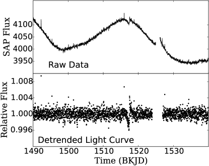
Figure 14: An example of a detrended light curve of KIC 10403228. The flare-like events are visible at several epochs. To create this curve, we generate 1000 light curves as described in the main text.

Now we move on to the comparison of the statistical property of stellar activities and the residuals of fit in Figure 9. Let us define $F_{\rm data}(t)$ as the flux ratio of the detrended light curve with respect to the mean. To investigate the short-term correlation of stellar activities, we divide the light curves into continuously brightening events $(F_{\rm data}(t)>1)$ and fading events $(F_{\rm data}(t)<1)$. Then, we compute the duration and amplitude (average of the deviation from the mean $|F_{\rm data}(t)-1|$) for each event. For comparison, we also calculate the duration and average relative flux for events in residuals in Figure 9. The left panel in Figure 15 is the scatter plot of the duration and average relative flux of events for three groups;

• all events out of the transit (the black data in Figure 14).

• residuals of the ringed-planet fit (the red line in Figure 9).

• residuals of the single-planet fit (the blue line in Figure 9).

The right panel in Figure 15 shows the distributions of durations for the three groups. In each duration bin, the vertical axis shows the total number of points in all events with that duration. The distribution of (a) is normalized to give the same total number of events as (b) and (c). The quoted error-bars are simply computed from Poisson statistics of the number of each event. Figure 15 shows that the distribution (b) is closer to (a) than (c). Thus, the ringed planet model is better than the planet model in terms of property of the correlated noise.

So far, we have shown that the ring-like anomaly cannot be explained statistically. We further consider whether the stellar noise can mimic the light-curve shape itself. We examine this hypothesis by focusing on the most significant fading event in the out-of-transit data; see the left panel of Figure 15. The light curve of this event is shown in Figure 16. We would like to see if the combination of the planet model and this event can reproduce the ringed-planet like feature. To do this, we appropriately embed the transit of the planet into the light curve around the fading event. Here, the parameters of the planet are the same as in Table 4. Then we fit the two models with and without a ring to those data, as shown in Figure 16 (b). As a result, we find the difference in $\chi^{2}$ of the two models to be $157.9$, which is smaller than $434.9$ obtained in Section 6.1 for solution 2. Thus, we conclude that it is difficult to reproduce the ring candidate by combining the stellar activities and the transit of the planet.

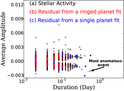
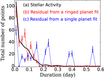
Figure 15: Statistical property of stellar activities of KIC10403228 and the residuals in Figure 9. (Left) Duration and average amplitude of continuously brighting $(F(t)>1)$ and fading $(F(t)<1)$ events are plotted. The black points are plotted from the stellar activities in Figure 14, and red points and blue points are plotted from the residuals of a ringed planet and a single planet model fitting in Figure 9 respectively. (Right) Histogram of duration. The color has the same meaning as in the left panel.

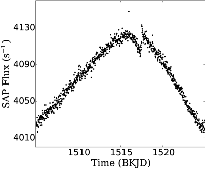
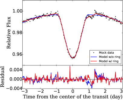
Figure 16: Testing the model of a transit of a planet with the stellar activities. (left) The most significant anomaly in KIC 10403228 as indicated with an arrow in the left panel of Figure 15. (right) The light curve of the transit of the planet embedded into the event in the left figure. The data are fitted with the ringed planet model (red) and the planet alone model (blue). The results show $\Delta\chi^{2}\simeq 157.9$, which is smaller than the real value $\Delta\chi^{2}=434.8$ in Section 6.1.

6.4.5 Combination of the above mechanisms

In principle, a combination of the mechanisms discussed above could be invoked to reproduce the observed anomaly. In Figure 13, for example, the bump and dip in the residual might be explained separately by a spot crossing and an exomoon. However, such a probability is a priori very low, and so we do not discuss those possibilities any further.

7 Conclusion and Future prospects

In this paper, we present a methodology to detect exoplanetary rings and apply it to the 89 long-period transiting planet candidates in the Kepler sample for the first time. After fitting a single planet model to light curves of target objects, we classify them into four groups depending on the observed anomalies and model predictions. Assuming grazing geometry and a titled ring, we obtain upper limits on $R_{\rm out}/R_{\rm p}$ for 12 planet candidates, and find $R_{\rm out}/R_{\rm p}<1.5$ for six of them. While we select five preliminary ringed planet candidates using the results of classification, four of them turn out to be false positives, but KIC 10403228 still remains as a possible ringed-planet system.

We fit our ringed planet model to the light curve of KIC 10403228, and we obtain two consistent solutions with the tilted ring. However, the V-shape of the current transit is a typical feature of an eclipsing binary, and the estimated orbital period $P$=450 years on the assumption of a circular orbit may be too long for the transit to be detected. Therefore, we also consider other two possibilities accounting for the data. One model assumes that the transit is caused by an eclipsing binary, and the ring-like feature is caused by a circumstellar disk rather than a planetary ring. For comparison, using the public code VESPA, we calculate the plausibility of this scenario and the planet scenario, and find that we cannot exclude both possibilities at the current stage. The other model we consider assumes the observed eclipse is caused by two objects orbiting around each other (hierarchical triple configuration), where the orbital motion of the smaller binary produces the long and asymmetric eclipse as observed for KIC 10403228. Assuming this model, we find various solutions for a wide range of orbital periods down to $P\simeq 1400\,\mathrm{days}$, although it requires more or less fine-tuned configurations. In addition to the above scenarios, we also discuss other possibilities, and find that none of them are likely to explain the data. In conclusion, there remain the three leading scenarios accounting for the data: “planetary ring scenario,” “circumstellar disk scenario,” and “hierarchical triple scenario.” A follow-up observation would play an important role in the further study.

The current research can be improved in several different ways. We can enlarge the sample of target objects towards those with shorter orbital periods. The interpretation of KIC 10403228 is fundamentally limited by the fact that it exhibits the only one transit. Obviously the credibility significantly increases if a system exhibits a robust ring-like anomaly repeatedly in the transits at different epochs. Moreover, difference in transit shapes at different epochs would enable us to discriminate between “disk scenario” and “hierarchical triple scenario.” In addition, our current methodology puts equal weights on the data points over the entire transit duration. Since the signature of a ring is particularly strong around the ingress and egress, more useful information on $R_{\rm out}/R_{\rm p}$ would be obtained with more focused analysis of the features around those epochs. We plan to improve our methodology, and attempt to apply it to a broader sample of transiting planets in due course. We do hope that we will be able to affirmatively answer a fundamental question “Are planetary rings common in the Galaxy?”.

Appendix A NUMERICAL INTEGRATION IN EQUATION (5)

We present a formulation for fast and accurate numerical integration of Equation (7). In addition to $(x,y)$ coordinates defined in Section 2, we also introduce the cylindrical coordinates $(r,\theta)$, whose origin is at the center of the star. The ranges of $(r,\theta)$ integration are $0<r<R_{\star}$ and $0\leq\theta<2\pi$. We integrate Equation (7) by dividing the total range of integration into several pieces as follows:

$$\int I(x,y)D(x,y)dS=\int^{R_{\star}}_{0}\int^{2\pi}_{0}I(\sqrt{1-(r/R_{\star})^{2}})D(r,\theta)rdrd\theta$$

$$=\sum_{i}\sum_{l}D_{i,l}\int_{r_{i}}^{r_{i+1}}\int_{\theta_{i,l}(r)}^{\theta_{i,l+1}(r)}I(\sqrt{1-(r/R_{\star})^{2}})rdrd\theta$$

$$=\sum_{i}\sum_{l}D_{i,l}\int_{r_{i}}^{r_{i+1}}(\theta_{i,l+1}(r)-\theta_{i,l}(r))I(\sqrt{1-(r/R_{\star})^{2}})rdr.$$ (A1)

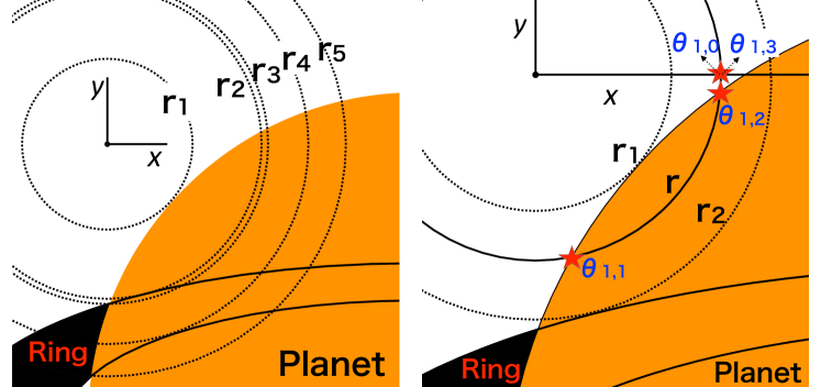
Figure 17: Illustrations of $r_{\rm i}$ (left) and $\theta_{i,j}(r)$ (right). A ringed planet is depicted with colors. In the figure, the boundary lines of rings behind the planet are expressed for clarity.

The intervals of integration are specified by $r_{\rm i}$ and $\theta_{i,j}(r)$. We will define them in the following, and the corresponding schematic illustration is depicted in Figure 17.

The number of the intersection points between a circle with the radius $r$ and the ringed planet depends on the value of $r$; there exists boundary values $r$ for the number of intersection points. We define $r_{i}$ as the $i$-th boundary value, and we arrange a set of $r_{i}$ in ascending order. If we have elements $r_{i}>R_{\star}$, we insert $R_{\star}$ into the set of $r_{i}$, and exclude elements that satisfy $r_{i}>R_{\star}$.

Next, let us suppose $r_{i}<r<r_{i+1}$, where the number of intersections remains the same. In this range, we define $\theta_{i,j}(r)$ to be the $j$-th value of $\theta$ of the intersection points between a ringed planet and a circle with the radius r. A set of $\theta_{i,j}(r)$ is also rearranged in ascending order, and we add $0,2\pi$ before and behind the set of $\theta_{i,j}(r)$. We define $D_{i,l}$ to be the values of $D(r,\theta,t)$ for $\theta_{i,l}(r)<\theta<\theta_{i,l+1}(r)$ and $r_{i}<r<r_{i+1}$. We will derive the equations for $r_{i}$ and $\theta_{i,j}(r)$ in the rest of appendix.

A.1 Derivation of $r_{i}$

Conditions for possible values of $r_{i}$ are divided into the following three cases:

• Intersections of the edge of the planet (circle) and the edge of the ring (ellipse).

• Extreme points of the distance function from the center of the star to the edge of the planet (circle).

• Extreme points of the distance function from the center of the star to the edge of the ring (ellipse).

The number of $r_{i}$ is at most eight for (a), two for (b), and two for (c). (a) and (b) are reduced to quadratic equations, which can be easily solved. The last case can be reduced to quartic equations. Here, we derive the quartic equations using the method of Lagrange multiplier. Let the length of the major axis be $2R$ and that of the minor axis be $2R(1-f)$, where $f$ is the oblateness. We set the center of the ellipse to be at $(x_{\rm p},y_{\rm p})$. For $(x,y)$ on the edge of the ellipse, we define the following function:

$$A(x,y,\lambda)=x^{2}+y^{2}+\lambda\left[\left(\frac{x-x_{\rm p}}{R}\right)^{2}+\left(\frac{y-y_{\rm p}}{R(1-f)}\right)^{2}-1\right].f$$ (A2)

From the condition, we need

$$\frac{\partial A}{\partial x} =2x+\frac{2(x-x_{p})\lambda}{R^{2}}=0$$ (A3)

$$\frac{\partial A}{\partial y} =2y+\frac{2(y-y_{p})\lambda}{(1-f)^{2}R^{2}}=0$$ (A4)

$$\frac{\partial A}{\partial\lambda} =\left(\frac{x}{R}\right)^{2}+\left(\frac{y}{R-Rf}\right)^{2}-1=0$$ (A5)

We reduce the above three equations to the following:

$$\frac{\lambda^{4}}{(1-f)^{4}R^{8}}+\frac{2\lambda^{3}}{(1-f)^{2}R^{4}}\left[\frac{1}{R^{2}}+\frac{1}{(1-f)^{2}R^{2}}\right]$$

$$+\lambda^{2}\left[\frac{1}{R^{4}}+\frac{4}{(1-f)^{2}R^{4}}+\frac{1}{(1-f)^{4}R^{4}}-\frac{x_{\rm p}^{2}}{(1-f)^{4}R^{6}}-\frac{y_{\rm p}^{2}}{(1-f)^{2}R^{6}}\right]$$

$$+\lambda\left[\frac{2}{R^{2}}+\frac{2}{(1-f)^{2}R^{2}}-\frac{x_{\rm p}^{2}+y_{\rm p}^{2}}{(1-f)^{2}R^{4}}\right]+1-\frac{x_{\rm p}^{2}}{R^{2}}-\frac{y_{\rm p}^{2}}{(1-f)^{2}R^{2}}=0.$$ (A6)

In general, quartic equations are analytically solved, but we compute the solutions for the equation using a root-finding algorithm, because of complexity of the analytic solution. $x$ and $y$ are calculated from derived $\lambda$ as follows:

$$x=\frac{-x_{\rm p}}{1+(\lambda/R^{2})}+x_{\rm p},\;y=\frac{-y_{\rm p}}{1+(\lambda/((1-f)R)^{2})}+y_{\rm p}.$$ (A7)

The number of solutions for $(x,y)$ is at most four. We exclude the solutions including complex numbers and/or $(x,y)$ not on the ellipse. Equation (A7) gives the singular solutions when

$$\lambda=-R^{2},\;-(1-f)^{2}R^{2}.$$ (A8)

Inserting the above values into Equation (A3) or (A4), we find $x_{\rm p}=0$ or $y_{\rm p}=0$. In this case, we cannot use Equation (A7), but the conditions are reduced to the quadratic equations, which can be easily solved.

A.2 Derivation of $\theta_{i,l}(r)$

To derive $\theta_{i,l}(r)$, we calculate the intersections of a circle, centered at $(0,0)$, with the radius $r$, and a transiting object, composed of the circle (planet) and two ellipses (rings). The center of the ring system is $(x_{\rm p},y_{\rm p})$. The intersections of two circles are easily computed and the number of the intersection points is two at most. Here, we derive the equations for intersection points of a circle and an ellipse. Let the radius of the circle be $r$. We select the same ellipse as before. For simplicity, we introduce the following parameters:

$$A=1-(1-f)^{2},\;B=2x_{\rm p}(1-f)^{2},$$

$$C=(1-f)^{2}R^{2}-r^{2}-(1-f)^{2}x_{\rm p}^{2}-y_{\rm p}^{2},\;D=-2y_{\rm p}.$$ (A9)

Then, an equation for $x$, the $x$-coordinate of intersections, is given by:

$$A^{2}x^{4}+2ABx^{3}+(2AC+B^{2}+D^{2})x^{2}+2BCx+C^{2}-D^{2}r^{2}=0,$$ (A10)

Equation (A10) is a quartic equation, which is analytically solved. We solve this equation with the root-finding method in the same way as before. The number of the solutions for this equation is four at most. In total, there are up to 10 possible solutions for $\theta_{i,l}(r)$.

A.3 Precision and computational time

To test the precision and the computational time in our scheme, we simulate a transit of a Saturn-like planet with $R_{\rm p}/R_{\star}=0.083667,\;R_{\rm in/p}=1.5,\;R_{\rm out/p}=2.0,\;\theta=\pi/3,\;\phi=\pi/3,\;T=1.0$. We take $P=10759.3$ days, $a/R_{\star}=2049.89$, $b=0.5$, $q_{1}=0.49$, and $q_{2}=0.34$ for orbital parameters and stellar parameters. For comparison, we prepare another integration scheme, which adopts pixel-by-pixel integration around the planetary center (e.g. Ohta et al. 2009).

First, we check the precision of the integration of our proposed method by comparing the precision of the pixel-by-pixel integration methods with $5000\times 5000$ pixels. As a result, two methods are in agreement to the extent of $10^{-7}$. Thus, our proposed method achieves the numerical error less than $10^{-7}$, which is much smaller than the typical noise in the Kepler data $10^{-4}$.

Second, we check the computational time of our template. Our proposed method typically takes $3.0$ ms for calculating one point and 200 s in fitting in Section 6.1. For comparison, we also check the computational time of the planetary transit using PyTransit package (Parviainen 2015), and we find that it takes 0.3 ms to compute all the 300 data points and 0.3 s in fitting in Section 6.1.

Finally, we compare our method with the pixel-by-pixel integration. If we set the pixel sizes to satisfy the same computational time as that of our method, the precision of the integration becomes $10^{-5}$ in the fiducial configurations. This precision depends on the specific configuration; it becomes $10^{-4}$ for if we adopt “$R_{\rm p}=0.17$ and $b=0.8$” and $3\times 10^{-6}$ for “$R_{\rm p}=0.042$ and $b=0.3$”. In summary, when we need a high-precision model, one should use our proposed method, and, if not, one may use the pixel-by-pixel integration to save the amount of calculation.

Incidentally, in a practical case of fitting with the Levenberg-Marquardt algorithm, our method is useful in a sense that gives the smooth value of $\chi^{2}$. This is because the smoothness is needed to calculate the differential values for $\chi^{2}$ in LM method.

Appendix B Method of target classification in Section 3

B.1 Concept

As we demonstrated in the main text, signatures of a ringed planet can be detected by searching for any deviation from the model light curve assuming a ringless planet. The deviation is, however, often very tiny and comparable to the noise level, and so careful quantitative arguments are required to discuss the presence or absence of the ring in a given light curve. In the following, we present a procedure to evaluate the detectability of a ring based on the comparison between the residual from the “planet-alone” model fit and the noise level in the light curve.

Let us denote one light curve including a transit by $I_{i}$ $(i=0,1,\cdots,N_{\rm data}$), where $N_{\rm data}$ is the number of data points. We also define $\delta_{i}$ as the residual of fitting $I_{i}$ with the planet-alone model. As a quantitative measure of this residual signal $\delta_{i}$ relative to the noise level, we introduce the following signal-to-noise ratio:

$$S/N=\frac{\sum_{i}\delta_{i}^{2}}{\sigma^{2}}=\frac{\sum_{i}\delta_{i}^{2}}{N_{\rm data}}\;\frac{N_{\rm data}}{\sigma^{2}}=\Delta^{2}\frac{1}{(\sigma/\sqrt{N_{\rm data}})^{2}}\;\;\;\;\;\;\left(\Delta^{2}\equiv\frac{\sum_{i}\delta_{i}^{2}}{N_{\rm data}}\right).$$ (B1)

In the last equality, we further define $\Delta^{2}$ as the variance of the residual time series, and $\sigma$ is evaluated as the standard deviation of the out-of-transit light curve. We use the subscript “obs” to specify the above quantities obtained by fitting the planet-alone model to the real observed data: $\delta_{i,\,\mathrm{obs}}$, $S/N_{\rm obs}$, and $\Delta^{2}_{\rm obs}$.

On the other hand, we can also compute the corresponding values of $\delta_{i}$, $S/N$, and $\Delta$, by fitting the simulated light curve of a ringed planet with the planet-alone model. We denote these values as $\delta^{2}_{i,\,\mathrm{sim}}(p)$, $S/N_{\rm sim}(p)$, and $\Delta^{2}_{\rm sim}(p)$, where $p$ represents the set of parameters of the ringed-planet model. If these values are sufficiently large compared to the noise variance (see $\Delta_{\rm thr}^{2}$ below), the signal of the ringed planet is distinguishable from the noise. In addition, comparing these theoretically expected residual levels with observed ones, we can relate the observed residuals to the parameters of the ringed model, even in the absence of clear anomalies.

To simplify the following arguments, we mainly use $\Delta^{2}$ instead of $S/N$ to evaluate the significance of the anomaly (see also Section B.3 for detailed reason). Practically, conversion from one to the other is rather simple, as the conversion factor $\sigma/\sqrt{N_{\rm data}}$ is well determined from the observed data alone; given a transit light curve, the transit duration $T_{\rm dur}$ and the bin size $t_{\rm bin}$ give the number of data points $N_{\rm data}=T_{\rm dur}/t_{\rm bin}$, and the standard deviation $\sigma$ can also be inferred from the out-of-transit flux.

For a given region of parameter space $p$, $\Delta^{2}_{\rm sim}(p)$ has the maximum value $\Delta^{2}_{\rm max,\,sim}$. If $\Delta^{2}_{\rm max,\,sim}$ is smaller than some threshold value $\Delta^{2}_{\rm thr}$ determined by the noise level in the light curve, the ringed-planets with the corresponding value of $p$, even if they exist, cannot be detected in the system. Then, the comparison of $\Delta^{2}_{\rm obs}$, $\Delta^{2}_{\rm max,\,sim}$, and $\Delta^{2}_{\rm thr}$ allows for classification into four categories schematically illustrated in Figure 18:

• : $\Delta^{2}_{\rm max,\,sim}<\Delta^{2}_{\rm thr}$
  The expected signal from the ring is so small compared to the noise level that we cannot discuss its detectability.

• : $\Delta^{2}_{\rm obs}<\Delta^{2}_{\rm thr}<\Delta^{2}_{\rm max,\,sim}$
  Although the rings with $\Delta^{2}_{\rm thr}<\Delta_{\rm sim}^{2}(p)$ could have been detected, no significant anomaly is observed ($\Delta_{\rm obs}<\Delta_{\rm thr}$) in reality. Thus, the parameter region that gives $\Delta^{2}_{\rm thr}<\Delta_{\rm sim}^{2}(p)$ is excluded.

• : $\Delta^{2}_{\rm thr}<\Delta^{2}_{\rm max,\,sim}<\Delta^{2}_{\rm obs}$
  A significant anomaly is detected, but its amplitude is too large to be explained by the ringed-planet model with the given range of $p$.

• : $\Delta^{2}_{\rm thr}<\Delta^{2}_{\rm obs}<\Delta^{2}_{\rm max,\,sim}$
  A significant anomaly is detected, and its amplitude is compatible with the ring model. In this case, we may find the ring parameters consistent with the observed anomaly.

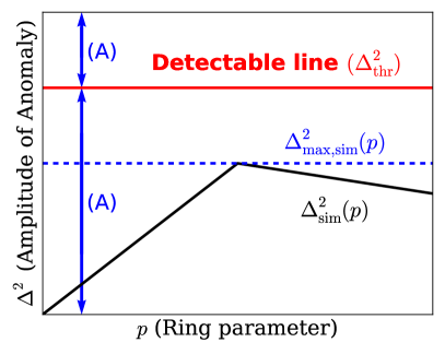
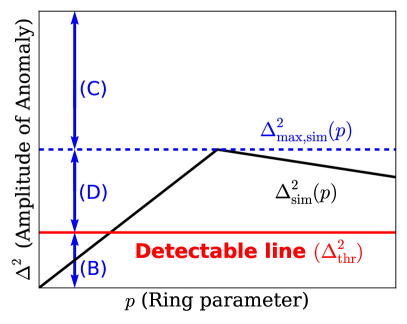
Figure 18: Classification using $\Delta^{2}_{\rm thr},\Delta^{2}_{\rm obs}$, and $\Delta_{\rm sim}^{2}(p)$. Candidates are classified into (A)$\sim$(D) depending on the value of $\Delta^{2}_{\rm obs}$. (Left) $\Delta^{2}_{\rm max,sim}<\Delta^{2}_{\rm thr}$. The detectability of rings is small. (Right) $\Delta^{2}_{\rm thr}<\Delta^{2}_{\rm max,sim}$. The detectability of rings is large.

The value of $\Delta^{2}_{\rm thr}$ is arbitrary. In this paper, we choose $\Delta^{2}_{\rm thr}$ so that it corresponds to $S/N=10$ in Equation (B1):

$$\Delta^{2}_{\rm thr}=\frac{10\,\sigma^{2}}{N_{\rm data}},$$ (B2)

where $\sigma$ and $N_{\rm data}$ are calculated from the observed data. The methods to calculate the other variances, $\Delta^{2}_{\rm obs}$, $\Delta^{2}_{\rm sim}(p)$, and $\Delta^{2}_{\rm max,\,sim}$ will be presented in the following subections.

Before proceeding further, let us consider the orbital period dependence of $N_{\rm data}=T_{\rm dur}/t_{\rm bin}$ in Equation (B1). From Kepler’s third law, $T_{\rm dur}\propto P\,(R_{\star}/a)\propto P^{1/3}$. For the short-period planets, $t_{\rm bin}\propto P$ because the number of folded transits is proportional to $1/P$. Thus, the number of the data $T_{\rm dur}/t_{\rm bin}$ is proportional to $P^{-2/3}$. This means that the detectability of rings ($S/N$) is higher for the shorter-period planets for a given value of $\Delta^{2}$. This explains the strong constraints on the ring parameters obtained by Heising et al. (2015) for hot Jupiters.

B.2 Calculation of $\Delta^{2}_{\rm obs}$

B.2.1 Definition

The residual $\delta_{i,\,\mathrm{obs}}$ is obtained by fitting the planet-alone model to the data. If the ring does not exist, the value of $S/N_{\rm obs}$ in Equation (B1), which is formally equivalent to the chi-squared, is expected to be close to the degree of freedom $DOF_{\rm obs}$. In contrary, if the ring does not exist, $S/N_{\rm sim}(p)$ is equal to zero. This mean that $S/N_{\rm obs}-S/N_{\rm sim}(p)\simeq DOF_{\rm obs}$ in the limit of the non-ring system. Thus, for comparison of $\Delta^{2}_{\rm sim}(p)$ and $\Delta^{2}_{\rm obs}$, the value of ($S/N-DOF_{\rm obs}$) serves as a good estimator of the observed anomaly rather than $S/N$. We thus slightly modify Equation (B1) to define $\Delta^{2}_{\rm obs}$ so that it corresponds to ($S/N-DOF_{\rm obs}$):

$$\Delta^{2}_{\rm obs} =\left(\chi^{2}-DOF_{\rm obs}\right)\frac{1}{(\sigma/\sqrt{N_{\rm data}})^{2}},$$ (B3)

where

$$\chi^{2} =\sum_{i}\left(\frac{\delta_{i,\,\mathrm{obs}}}{\sigma}\right)^{2}.$$ (B4)

The residual $\delta_{i,\,{\rm obs}}$ is defined for the best-fit planet-alone model obtained by minimizing $\chi^{2}$ as described in Section B.2.2 below. The value of $\chi^{2}$ is computed using the data just around the transit (within $0.6\,T_{\rm dur}$ from the transit center) so that the value is not strongly affected by the out-of-transit data. We assume $DOF_{\rm obs}=N_{\rm data}-N_{\rm para}-1$, where $N_{\rm para}$ is the number of fitted parameters.

B.2.2 Detail of fitting

In fitting, we minimize $\chi^{2}$ using the Levenberg-Marquardt algorithm by implementing cmpfit (Markwardt 2009). The adopted model $M(t)$ is composed of a fourth-order polynomial and a transit model $F(t)$:

$$M(t)=F(t)[c_{0}+c_{1}(t-T_{0})+c_{2}(t-T_{0})^{2}+c_{3}(t-T_{0})^{3}+c_{4}(t-T_{0})^{4}],$$ (B5)

where $c_{i}$ are coefficients of polynomials, and $T_{0}$ is a time offset. The polynomials are used to remove the long-term flux variations in the light curve. The transit model $F(t)$ is implemented by the PyTransit package (Parviainen 2015). PyTransit generates the light curves based on the model of Mandel & Agol (2002) with the quadratic limb darkening law.

The above model $M(t)$ includes 12 parameters, $t_{0},R_{\rm p}/R_{\star},b,a/R_{\star},P,q_{1},q_{2}$, and $c_{i}\,(i=0\sim 4)$. For KOIs, the initial values of $a/R_{\star},R_{\rm p}/R_{\star},$ and $b$ for fitting are taken from the KOI catalog. The initial values of the limb darkening parameters are taken from the Kepler Input Catalog. For a single transit event, where we cannot estimate the orbital period from the transit interval, we choose $P$, instead of $a/R_{\star}$, as a fitting parameter and estimate $a/R_{\star}$ from $P$ using Kepler’s third law and the mean stellar density given in the catalog.

In fitting, we remove outliers iteratively to correctly evaluate $\chi^{2}$. We first fit all the data with the model $M(t)$, and flag the points that deviate more than $5\sigma$ from the best model. We then refit only the non-flagged data using the same model, and update the flags of all the original data points, including the ones classified as outliers before, on the basis of the new best model and the same $5\sigma$ criterion. We iterate this procedure until the flagged data are converged. While this process gives a more robust evaluation of $\chi^{2}$, it may also erase the signature of the ringed planet; thus we visually check all the light curves in any case not to miss the real ringed planets.

The noise variance $\sigma^{2}$ is estimated for each transit light curve by fitting the out-of-transit light curve with a fourth-order polynomial, and calculating the variance of the residuals. Flare-like events are excluded from the estimation of the noise variance.

B.3 Calculation of $\Delta^{2}_{\rm sim}(p)$ and $\Delta^{2}_{\rm sim,max}$

Since the parameter space $p$ for a ringed planet is very vast, we wish to reduce the volume we need to search with simulations as much as possible. First we show that $\Delta^{2}_{\rm sim}(p)$ does not depend on $P$ and $a/R_{\star}$ with other parameters fixed including limb darkening parameters $q_{1},q_{2}$, the transit impact parameter $b$, planet-to-star radius ratio $R_{\rm p}/R_{\star}$, inner and outer ring radii relative to the planetary radius $r_{\rm in/p}$ and $r_{\rm out/p}$, , the direction of the ring $(\theta,\phi)$, and a shading parameter $T$. This property becomes apparent by rewriting $\Delta^{2}_{\rm sim}(p)$ into the following integral form approximately, assuming that the sampling rate ($t_{\rm bin}$) is sufficiently small compared to the duration $T_{\rm dur}$:

$$\Delta_{\rm sim}^{2}(p)\simeq\frac{\int_{-T_{\rm dur}/2}^{T_{\rm dur}/2}\delta_{\rm sim}^{2}(t,p)dt}{\int_{-T_{\rm dur}/2}^{T_{\rm dur}/2}dt}=\frac{\int_{-1/2}^{1/2}\delta_{\rm sim}^{2}(T_{\rm dur}t^{\prime},p)dt^{\prime}}{\int_{-1/2}^{1/2}dt^{\prime}}=\int_{-1/2}^{1/2}\bar{\delta}_{\rm sim}^{2}(t^{\prime},p)dt^{\prime},$$ (B6)

where

$$\bar{\delta}_{\rm sim}(t,p)\equiv\delta_{\rm sim}(T_{\rm dur}t,p)$$ (B7)

and the origin of time is shifted to the transit center. Assuming that the values of $q_{1}$, $q_{2}$, $b$, $R_{\rm p}/R_{\star}$, $r_{\rm out/p}$, $r_{\rm in/p}$, $\theta$, $\phi$, and $T$ are fixed, $\bar{\delta}(t,p)$ defined above does not depend on $T_{\rm dur}$ explicitly. Therefore, $\Delta_{\rm sim}^{2}(p)$ given by Equation (B6) does not depend on the time scale of the transit $T_{\rm dur}$, which is determined by $P$ and $a/R_{\star}$, and we do not need to simulate the dependence of $\Delta_{\rm sim}^{2}(p)$ on these two parmeters.

To constrain the parameter space further, we use the observed transit depth. Here we also assume that the values of $q_{1}$, $q_{2}$, $b$, $T$, $r_{\rm in/p}$, and the ring direction are fixed and that $R_{\rm p}/R_{\star}$ and $r_{\rm out/p}$ are the only free parameters. Then, the constraint on the observed transit depth leaves only one degree of freedom, specified by contours in the $R_{\rm p}/R_{\star}$-$r_{\rm out/p}$ plane; henceforth we rewrite $\Delta_{\rm sim}^{2}(p)$ as $\Delta^{2}_{\rm sim}(r_{\rm out/p})$ to explicitly show this dependence.

To compute the relation $\Delta^{2}_{\rm sim}(r_{\rm out/p})$ for a given transit depth, we first calculate the value of $\Delta^{2}_{\rm sim}$ and the transit depths for a sufficient number of points in the $(r_{\rm out/p},R_{\rm p}/R_{\star})$ plane. The necessary number of points depends on the fiducial model, and, in our simulation, we prepare about two hundred points for each model in Table 2. For any $r_{\rm out/p}$, the observed transit depth uniquely translates into $R_{\rm p}/R_{\star}$ by the interpolation in the $R_{\rm p}/R_{\star}$-transit depth plane, because the transit depth is a monotonically increasing function of the $R_{\rm p}/R_{\star}$. Thus, the given value of $r_{\rm out/p}$ is uniquely related to $\Delta^{2}_{\rm sim}$ given the transit depth. By repeating this procedure for many different values of $r_{\rm out/p}$, we can compute the relation $\Delta^{2}_{\rm sim}(r_{\rm out/p})$. We note that once a sufficient number of interpolated lines are prepared, one transit depth determines the relation $\Delta^{2}_{\rm sim}(r_{\rm out/p})$ without additional calculation.

Figure 19 shows $\Delta^{2}_{\rm sim}(r_{\rm out/p})$ curves created in this way, for $4\times 4=16$ different sets of impact parameters, ring directions, and transit depths. The four sets of $p$ adopted here (model I $\sim$ model IV) are summarized in Table 2, and four transit depths are chosen to be 0.001, 0.005, 0.01, and 0.05. We fix $T=1$ and $r_{\rm in/p}=1$ in all of these simulations.

Here we simulate $\Delta^{2}_{\rm sim}(r_{\rm out/p})$ only for $1\leq r_{\rm out/p}\leq r_{\rm eq}$, where $r_{\rm eq}$ is the value of $r_{\rm out/p}$ for which the minor axis of the sky-projected outer ring is equal to the planetary radius, computed for each model. This is because the value of $\Delta^{2}_{\rm sim}(r_{\rm out/p})$ shows no $R_{\rm p}/R_{\star}$ dependence beyond $r_{\rm eq}$, when $T=1$ and $r_{\rm in/p}=1$ are adopted; if this is the case, the planetary disk is within the outer disk and the transit depth is solely determined by the latter.

In this paper, we only use the observed constraint on the transit depth. However, this is just for simplicity and we can certainly take into account the constraints on other parameters including $b$, $q_{1}$, and $q_{2}$ from the morphology of the observed transit light curve (e.g. egress and ingress durations). Such constraints further restrict the ring models that could be consistent with the observed light curve and thus help more elaborate discussions on the ring parameters, which we leave to future works.

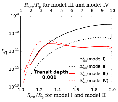
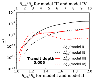
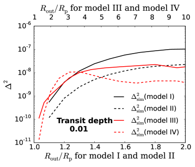
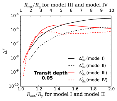
Figure 19: The value of $\Delta^{2}_{\rm sim}(p)$ as a function of $r_{\rm out/p}$ for four different transit depths. The four lines in each panel correspond to four different sets of parameters (model I $\sim$ model IV) summarized in Table 2.

Appendix C Derivation of the upper limit of $r_{\rm out/p}$: case of KOI-1466.01

If a system is classified into group (B), the ring models with $\Delta^{2}_{\rm thr}<\Delta_{\rm sim}^{2}(r_{\rm out/p})$ are excluded. The upper limits of $r_{\rm out/p}$ thus obtained are summarized in Sections 4 and 5. Here we describe how the limit is derived using the relation $\Delta^{2}_{\rm sim}(r_{\rm out/p})$, taking KOI-1466.01 for example.

The black and red lines in Figure 20 are theoretically expected signals from the ringed planets (i.e., $\Delta^{2}_{\rm sim}(r_{\rm out/p})$) for model I $\sim$ model IV and for the transit depth of 0.0202 inferred from the observed data. The green line shows the threshold value of $\Delta^{2}_{\rm thr}$ that satisfies $S/N=10$, and the blue line shows the observed residual level $\Delta^{2}_{\rm obs}$ obtained by fitting the planet-alone model to the data. Here $\Delta^{2}_{\rm obs}<\Delta^{2}_{\rm thr}$, which means that no significant deviation from the planet-alone model is detected. In this case, we can in turn exclude the models above the green line, because any anomaly above this level should have been detected if present. In the case of the black solid line (model I), for example, the ring with $r_{\rm out/p}>1.5$ would have produced the anomaly with $S/N>10$, which is not detected in reality. Thus, we can set the upper limit of $r_{\rm out/p}<1.5$ for model I. Note that the upper limits depend on the adopted parameter set; this situation is clearly illustrated in Figure 20, where similar limits cannot be derived for the other models.

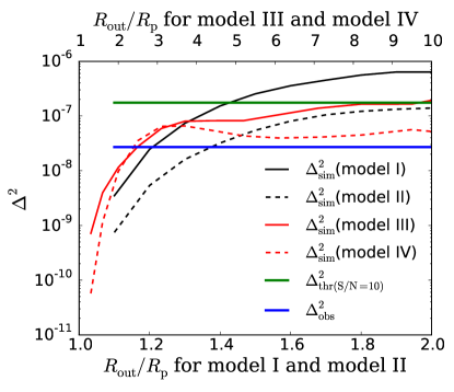
Figure 20: Derivation of the upper limit of $r_{\rm out/p}$ in the case of KOI-1466.01. The observed signature of the ring in the blue line is small compared with the detectability of the ring shown in the green line. The red and black lines are the theoretically expected values of $\Delta^{2}$ for models I-IV in Table 2. Assuming model I (black solid line), for example, the region with $1.5<r_{\rm out/p}$ (i.e. a part of the line above the green line) is inconsistent with the non-detection of the anomaly and thus excluded.

References

- Arnold & Schneider (2004) Arnold, L., & Schneider, J. 2004, A&A, 420, 1153
- Barnes & Fortney (2004) Barnes, J. W., & Fortney, J. J. 2004, ApJ, 616, 1193
- Barnes et al. (2011) Barnes, J. W., Linscott, E., & Shporer, A. 2011, ApJS, 197, 10
- Benomar et al. (2014) Benomar, O., Masuda, K., Shibahashi, H., & Suto, Y. 2014, PASJ, 66, 94
- Brogi et al. (2016) Brogi, M., de Kok, R. J., Albrecht, S., et al. 2016, ApJ, 817, 106
- Brown et al. (2001) Brown, T. M., Charbonneau, D., Gilliland, R. L., Noyes, R. W., & Burrows, A. 2001, ApJ, 552, 699
- Carter & Winn (2010) Carter, J. A., & Winn, J. N. 2010, ApJ, 716, 850
- Clanton & Gaudi (2016) Clanton, C., & Gaudi, B. S. 2016, The Astrophysical Journal, 819, 125
- Coughlin et al. (2016) Coughlin, J. L., Mullally, F., Thompson, S. E., et al. 2016, ApJS, 224, 12
- Cox (2000) Cox, A. N. 2000, Allen’s astrophysical quantities
- Dotter et al. (2008) Dotter, A., Chaboyer, B., Jevremović, D., et al. 2008, The Astrophysical Journal Supplement Series, 178, 89
- Dressing & Charbonneau (2013) Dressing, C. D., & Charbonneau, D. 2013, The Astrophysical Journal, 767, 95
- Dyudina et al. (2005) Dyudina, U. A., Sackett, P. D., Bayliss, D. D. R., et al. 2005, ApJ, 618, 973
- Hayashi (1981) Hayashi, C. 1981, Progress of Theoretical Physics Supplement, 70, 35
- Heising et al. (2015) Heising, M. Z., Marcy, G. W., & Schlichting, H. E. 2015, ApJ, 814, 81
- Huber et al. (2013) Huber, D., Chaplin, W. J., Christensen-Dalsgaard, J., et al. 2013, ApJ, 767, 127
- Janson et al. (2012) Janson, M., Hormuth, F., Bergfors, C., et al. 2012, The Astrophysical Journal, 754, 44
- Kenworthy & Mamajek (2015) Kenworthy, M. A., & Mamajek, E. E. 2015, ApJ, 800, 126
- Kipping (2010) Kipping, D. M. 2010, MNRAS, 408, 1758
- Kipping (2013) —. 2013, MNRAS, 435, 2152
- Lainey et al. (2012) Lainey, V., Karatekin, Ö., Desmars, J., et al. 2012, ApJ, 752, 14
- Maeder (2009) Maeder, A. 2009, Physics, Formation and Evolution of Rotating Stars, doi:10.1007/978-3-540-76949-1
- Mandel & Agol (2002) Mandel, K., & Agol, E. 2002, ApJ, 580, L171
- Markwardt (2009) Markwardt, C. B. 2009, in Astronomical Society of the Pacific Conference Series, Vol. 411, Astronomical Data Analysis Software and Systems XVIII, ed. D. A. Bohlender, D. Durand, & P. Dowler, 251
- Masuda (2015) Masuda, K. 2015, ApJ, 805, 28
- Morton (2012) Morton, T. D. 2012, ApJ, 761, 6
- Morton (2015) —. 2015, VESPA: False positive probabilities calculator, Astrophysics Source Code Library, ascl:1503.011
- Ohta et al. (2005) Ohta, Y., Taruya, A., & Suto, Y. 2005, ApJ, 622, 1118
- Ohta et al. (2009) —. 2009, ApJ, 690, 1
- Parviainen (2015) Parviainen, H. 2015, MNRAS, 450, 3233
- Queloz et al. (2000) Queloz, D., Eggenberger, A., Mayor, M., et al. 2000, A&A, 359, L13
- Rappaport et al. (2014) Rappaport, S., Swift, J., Levine, A., et al. 2014, ApJ, 788, 114
- Sanchis-Ojeda et al. (2011) Sanchis-Ojeda, R., Winn, J. N., Holman, M. J., et al. 2011, ApJ, 733, 127
- Santos et al. (2015) Santos, N. C., Martins, J. H. C., Boué, G., et al. 2015, A&A, 583, A50
- Schlichting & Chang (2011) Schlichting, H. E., & Chang, P. 2011, ApJ, 734, 117
- Schneider (1999) Schneider, J. 1999, Academie des Sciences Paris Comptes Rendus Serie B Sciences Physiques, 327, 621
- Schwarz et al. (2016) Schwarz, H., Ginski, C., de Kok, R. J., et al. 2016, ArXiv e-prints, arXiv:1607.00012
- Snellen et al. (2014) Snellen, I. A. G., Brandl, B. R., de Kok, R. J., et al. 2014, Nature, 509, 63
- Uehara et al. (2016) Uehara, S., Kawahara, H., Masuda, K., Yamada, S., & Aizawa, M. 2016, ApJ, 822, 2
- Wang et al. (2015) Wang, J., Fischer, D. A., Barclay, T., et al. 2015, ApJ, 815, 127
- Zhou et al. (2016) Zhou, Y., Apai, D., Schneider, G. H., Marley, M. S., & Showman, A. P. 2016, ApJ, 818, 176
- Zuluaga et al. (2015) Zuluaga, J. I., Kipping, D. M., Sucerquia, M., & Alvarado, J. A. 2015, ApJ, 803, L14