Hessian corrections to Hybrid Monte Carlo

Abstract

A method for the introduction of second-order derivatives of the log likelihood into HMC algorithms is introduced, which does not require the Hessian to be evaluated at each leapfrog step but only at the start and end of trajectories.

1 Introduction

Markov chain Monte Carlo (MCMC) is a highly influential computationally intensive method for performing Bayesian inference, with a large variety of applications (Brooks et al., 2011). While earlier MCMC algorithms made use of random walks in parameter space (Gilks et al., 1995), as highlighted in a recent review by Green et al. (2015), the use of derivatives can lead to improved algorithms.

One derivative-based approach is HMC, standing for either Hybrid (Duane et al., 1987) or Hamiltonian (Neal, 2011) Monte Carlo, which requires first derivatives of the log likelihood to be available. More recently, second derivatives have been included via the use of geometric approaches (Girolami and Calderhead, 2011, Betancourt, 2013). This working paper introduces a different route to inclusion of second-order derivatives through truncated Taylor expansion of the log-likelihood, after which Hamilton’s equations can be solved exactly without further approximation. This algorithm is called HHMC (for Hessian-corrected HMC) and is able to sample accurately from distributions with different scales for each parameter, which is challenging for standard HMC.

2 A Hessian HMC algorithm

2.1 Local solution of Hamilton’s equations

The idea behind HMC is to propose a new set of parameters $\boldsymbol{\theta}^{*}$ starting from $\boldsymbol{\theta}^{n}$ by making use of additional ‘momentum’ variables $\mathbf{p}$. We will consider the general case where $\mathbf{p}^{n}\sim\mathcal{N}(\mathbf{q},\mathbf{Q})$ in general, although in standard HMC, $\mathbf{q}=\mathbf{0}$ and $\mathbf{Q}=\mathbbm{1}$.

Supposing our aim is to sample according to $\pi$, and we let $l=\mathrm{ln}(\pi)$, then the basis for HMC algorithm design is Hamilton’s equations. These make use of the Hamiltonian

$$\mathcal{H}=\frac{1}{2}\mathbf{p}^{2}-l\text{ ,}$$ (1)

and take the form

$$\frac{\mathrm{d}\boldsymbol{\theta}}{\mathrm{d}t}=\frac{\partial\mathcal{H}}{\partial\mathbf{p}}=\mathbf{p}\text{ ,}\qquad\frac{\mathrm{d}\mathbf{p}}{\mathrm{d}t}=-\frac{\partial\mathcal{H}}{\partial\boldsymbol{\theta}}=\boldsymbol{\partial}l\text{ .}$$ (2)

In general, these cannot be solved analytically and so proposals are made on the basis of a numerical approximation, for example the leapfrog method, in which $L$ steps of length $\varepsilon$ are

$$\boldsymbol{\theta}_{0} =\boldsymbol{\theta}^{n}\text{ ,}$$ (3)

$$\mathbf{p}_{1/2} =\mathbf{p}^{n}+\frac{\varepsilon}{2}\boldsymbol{\partial}l(\boldsymbol{\theta}^{n})\text{ ,}$$

$$\boldsymbol{\theta}_{i} =\boldsymbol{\theta}_{i-1}+\varepsilon\mathbf{p}_{i-(1/2)}\text{ ,}\quad i\in\{1,\ldots L\}\text{ ,}$$

$$\mathbf{p}_{i+(1/2)} =\mathbf{p}_{i-(1/2)}+\varepsilon\boldsymbol{\partial}l(\boldsymbol{\theta}_{i})\quad i\in\{1,\ldots L-1\}\text{ ,}$$

$$\boldsymbol{\theta}^{*} =\boldsymbol{\theta}_{L}\text{ ,}$$

$$\mathbf{p}^{*} =\mathbf{p}_{L-(1/2)}+\frac{\varepsilon}{2}\boldsymbol{\partial}l(\boldsymbol{\theta}^{*})\text{ .}$$

This algorithm, together with the initial random choice of $\mathbf{p}^{n}$, defines a marginal proposal density $\rho(\boldsymbol{\theta}^{*}|\boldsymbol{\theta}^{n})$. This will be close to the solution of (2) over a time period $\delta:=\varepsilon L$ for large $L$ and small $\varepsilon$.

Now suppose that we approximate $l=\mathrm{ln}(\pi)$ in the neighbourhood of some value $\boldsymbol{\theta}^{n}$ through Taylor expansion

$$l(\boldsymbol{\theta}^{n}+\mathbf{x})\approx l(\boldsymbol{\theta}^{n})+\mathbf{v}^{\!\top}\mathbf{x}+\frac{1}{2}\mathbf{x}^{\!\top}\mathbf{H}\mathbf{x}\text{ ,}$$ (4)

where

$$v_{i}:=\left.\frac{\partial l}{\partial\theta^{i}}\right|_{\boldsymbol{\theta}^{n}}\text{ ,}\quad H_{ij}:=\left.\frac{\partial^{2}l}{\partial\theta^{i}\partial\theta^{j}}\right|_{\boldsymbol{\theta}^{n}}\text{ ,}\quad\mathbf{v}:=(v_{i})\text{ ,}\quad\mathbf{H}:=(H_{ij})\text{ .}$$ (5)

Then we can approximate Hamilton’s equations in the region of $\boldsymbol{\theta}^{n}$ through the linear SDE

$$\mathrm{d}\mathbf{x}=\left(\mathbf{A}\mathbf{x}+\mathbf{b}\right)\mathrm{d}t\text{ ,}$$ (6)

where

$$\mathbf{x}=\begin{pmatrix}\boldsymbol{\theta}\\ \mathbf{p}\end{pmatrix}\text{ ,}\quad\mathbf{A}=\begin{pmatrix}\mathbf{0}&\mathbbm{1}\\ \mathbf{H}&\mathbf{0}\end{pmatrix}\text{ ,}\quad\mathbf{b}=\begin{pmatrix}\mathbf{0}\\ \mathbf{v}\end{pmatrix}\text{ .}\quad$$ (7)

Note that this SDE does not have a white-noise term, but is nevertheless a special case of the results of Archambeau et al. (2007), and therefore has Gaussian solution with mean $\mathbf{m}$ and covariance matrix $\mathbf{S}$ obeying

$$\frac{\mathrm{d}\mathbf{m}}{\mathrm{d}t}=\mathbf{A}\mathbf{m}+\mathbf{b}\text{ ,}\qquad\frac{\mathrm{d}\mathbf{S}}{\mathrm{d}t}={\mathbf{A}}\mathbf{S}+\mathbf{S}\mathbf{A}^{\!\top}\text{ ,}\qquad\mathbf{m}(0)=\begin{pmatrix}\boldsymbol{\theta}^{n}\\ \mathbf{q}\end{pmatrix}\text{ ,}\qquad\mathbf{S}(0)=\begin{pmatrix}\mathbf{0}&\mathbf{0}\\ \mathbf{0}&\mathbf{Q}\end{pmatrix}\text{ .}$$ (8)

Solving these ODEs over the interval $[0,\delta]$ gives, after some analytic work,

$$\mathrm{Mean}(\boldsymbol{\theta}^{*}(\delta)) =\left(\mathrm{cosh}\left(\mathbf{H}^{1/2}\delta\right)-\mathbbm{1}\right)\mathbf{H}^{-1}\mathbf{q}\text{ ,}$$ (9)

$$\mathrm{Cov}(\boldsymbol{\theta}^{*}(\delta)) =\mathbf{H}^{-1/2}\mathrm{sinh}\left(\mathbf{H}^{1/2}\delta\right)\mathbf{Q}\mathbf{H}^{-1/2}\mathrm{sinh}\left(\mathbf{H}^{1/2}\delta\right)\text{ .}$$

If we then impose that this should correspond to a situaion where the marginal proposal $\rho(\boldsymbol{\theta}^{*}|\boldsymbol{\theta}^{n})=\pi(\boldsymbol{\theta}^{*})$ under the approximation (4), then we obtain a solution for the proposal distribution after additional analytic work:

$$\mathbf{q}(\boldsymbol{\theta}^{n})=\mathrm{cosh}\left(\mathbf{H}^{1/2}\delta\right)\mathbf{H}^{-1/2}\left(\mathrm{sinh}\left(\mathbf{H}^{1/2}\delta\right)\right)^{-1}\boldsymbol{\partial}l\text{ ;}\qquad\mathbf{Q}(\boldsymbol{\theta}^{n})=-\left(\mathrm{sinh}\left(\mathbf{H}^{1/2}\delta\right)\right)^{-2}\text{ .}$$ (10)

In terms of numerical computation of (10), despite the seeming complexity of the matrix functions, the general approach of Davies and Higham (2003) is applicable. In particular, despite the appearance of fractional powers in the compact expression (10), all of the functions involved have only integer matrix powers in their Taylor series and so is expressible as matrix polynomials.

Note that we can no longer write the accept-reject probabilities in this algorithm in terms of the Hamiltonian, however since the leapfrog integrator (3) is reversible it is still possible to calculate these probabilities. In particular, if we start with $\boldsymbol{\theta}^{n},\mathbf{p}^{n}$ and propose $\boldsymbol{\theta}^{*},\mathbf{p}^{*}$,

$$\frac{\rho(\boldsymbol{\theta}^{n},\mathbf{p}^{n}|\boldsymbol{\theta}^{*},\mathbf{p}^{*})}{\rho(\boldsymbol{\theta}^{*},\mathbf{p}^{*}|\boldsymbol{\theta}^{n},\mathbf{p}^{n})}=\frac{\mathcal{N}(-\mathbf{p}^{*}|\mathbf{q}(\boldsymbol{\theta}^{*}),\mathbf{Q}(\boldsymbol{\theta}^{*}))}{\mathcal{N}(\mathbf{p}^{n}|\mathbf{q}(\boldsymbol{\theta}^{n}),\mathbf{Q}(\boldsymbol{\theta}^{n}))}$$ (11)

The MCMC algorighm based on (10) and (11) is called HHMC for Hessian-corrected HMC. This algorithm does not require the Hessian $\mathbf{H}$ at each leapfrog step, just at the start and end of trajectories, and does not involve third-order derivatives $\partial_{i}\mathbf{H}$ making it much less computationally costly than Riemannian approaches (Girolami and Calderhead, 2011, Betancourt, 2013).

3 A target distribution with heterogeneous scales

Following Neal (2012), consider the following multivariate Gaussian target density:

$$\pi(\boldsymbol{\theta})=\mathcal{N}(\boldsymbol{\theta}|\mathbf{0};\mathbf{V})\text{,}$$ (12)

where $\mathbf{V}$ is a diagonal matrix with entries equal to the squares of: 110; 100; twenty-six evenly spaced standard deviations between 16 and 8; 1.1; and 1.0. Neal suggests this distribution as a diagnostic for HMC because the variable scales associated with each parameter create difficulties for the algorithm.

Running MCMC chains of length $10^{3}$ using $L=10$ leapfrog steps each with a step size of $\epsilon=0.2$ for HMC and HHMC gives the results shown in Figures 1, 2, 3 and 4. The results show that HMC is out-performed by HHMC.

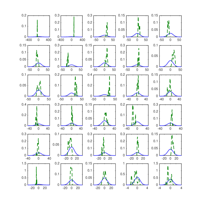
Figure 1: Given a multivariate normal target density (blue solid lines) with variable scales, HMC (green dashed lines) does poorly.

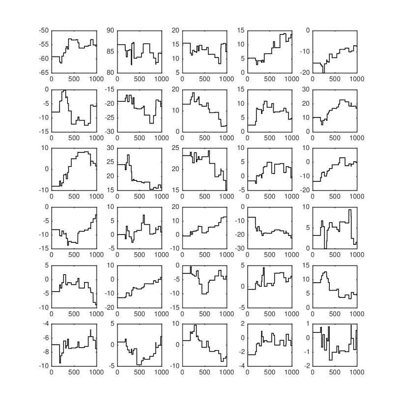
Figure 2: HMC trace plots.

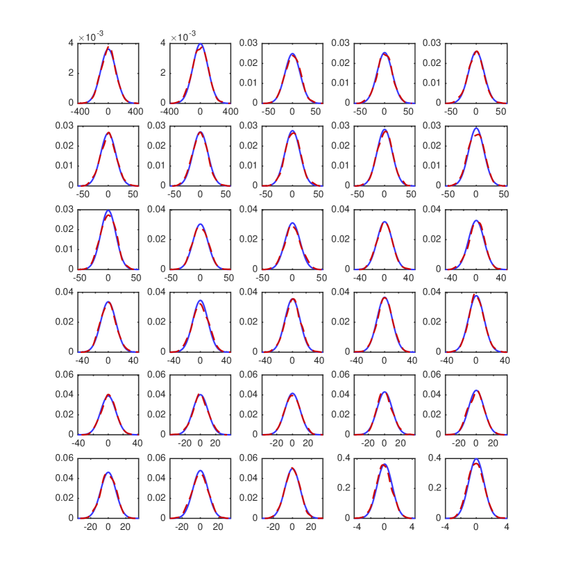
Figure 3: Given a multivariate normal target density (blue solid lines) with variable scales, HHMC (red dashed lines) does well.

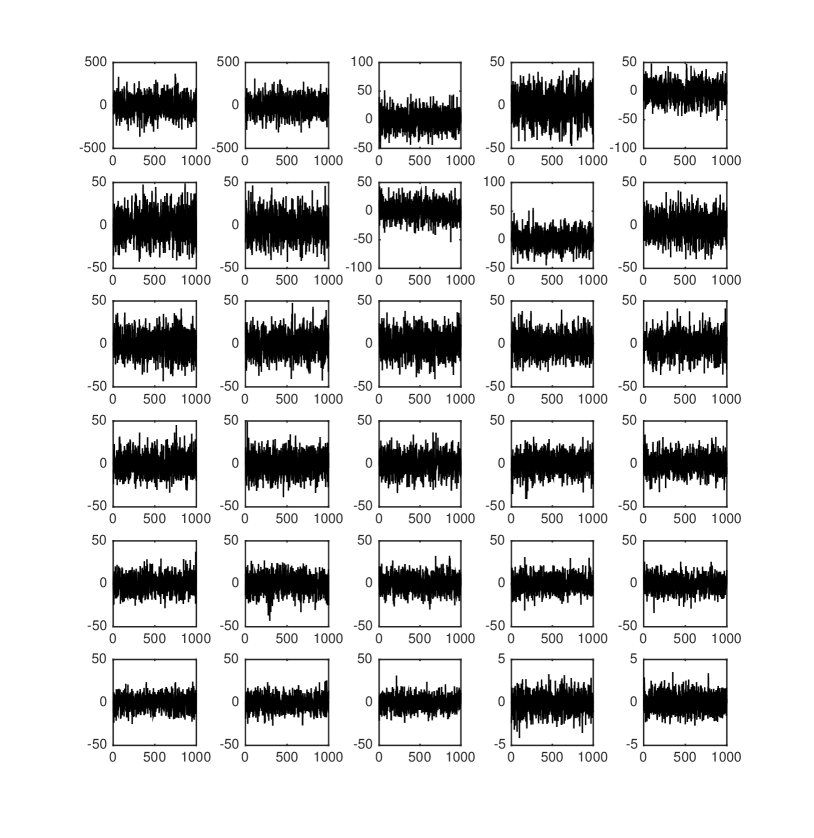
Figure 4: HHMC trace plots.

References

• Archambeau et al. (2007) C. Archambeau, D. Cornford, M. Opper, and J. Shawe-Taylor. Gaussian process approximations of stochastic differential equations. Journal of Machine Learning Research–Proceedings Track, 1:1–16, 2007.
• Betancourt (2013) M. Betancourt. A general metric for Riemannian manifold Hamiltonian Monte Carlo. In F. Nielsen and F. Barbaresco, editors, Geometric Science of Information, volume 8085 of Lecture Notes in Computer Science, pages 327–334. Springer Berlin Heidelberg, 2013.
• Brooks et al. (2011) S. Brooks, A. Gelman, G. L. Jones, and X.-L. Meng, editors. Handbook of Markov Chain Monte Carlo. CRC Press, 2011.
• Davies and Higham (2003) P. I. Davies and N. J. Higham. A Schur-Parlett algorithm for computing matrix functions. SIAM Journal on Matrix Analysis and Applications, 25(2):464–485, 2003.
• Duane et al. (1987) S. Duane, A. Kennedy, B. J. Pendleton, and D. Roweth. Hybrid monte carlo. Physics Letters B, 195(2):216–222, 1987.
• Gilks et al. (1995) W. R. Gilks, S. Richardson, and D. J. Spiegelhalter. Markov Chain Monte Carlo in Practice. Chapman and Hall/CRC, 1995.
• Girolami and Calderhead (2011) M. Girolami and B. Calderhead. Riemann manifold Langevin and Hamiltonian Monte Carlo methods. Journal of the Royal Statistical Society, Series B, 73(2):123–214, 2011.
• Green et al. (2015) P. J. Green, K. Łatuszyński, M. Pereyra, and C. P. Robert. Bayesian computation: a summary of the current state, and samples backwards and forwards. Statistics and Computing, 25(4):835–862, 2015.
• Neal (2011) R. M. Neal. MCMC using Hamiltonian dynamics. In S. Brooks, A. Gelman, G. L. Jones, and X.-L. Meng, editors, Handbook of Markov Chain Monte Carlo, chapter 5. CRC Press, 2011.
• Neal (2012) R. M. Neal. No U-turns for Hamiltonian Monte Carlo – comments on a paper by Hoffman and Gelman. https://radfordneal.wordpress.com/2012/01/21/no-u-turns-for-hamiltonian-monte-carlo-comments-on-a-paper-by-hoffman-and-gelman/ (Accessed 27 February 2017), 2012.
Refer to caption