Multigrid methods based on shifted inverse iteration for the Maxwell eigenvalue problem

Abstract

In this paper two types of multgrid methods, i.e., the Rayleigh quotient iteration and the inverse iteration with fixed shift, are developed for solving the Maxwell eigenvalue problem with discontinuous relative magnetic permeability and electric permittivity. With the aid of the mixed form of source problem associated with the eigenvalue problem, we prove the uniform convergence of the discrete solution operator to the solution operator in $\mathbf{L}^{2}(\Omega)$ using discrete compactness of edge element space. Then we prove the asymptotically optimal error estimates for both multigrid methods. Numerical experiments confirm our theoretical analysis.

1 Introduction

The Maxwell eigenvalue problem is of basic importance in designing resonant structures for advanced waveguide. Up to now, the communities from numerical mathematics and computational electromagnetism have developed plenty of numerical methods for solving this problem (see, e.g., [1, 3, 4, 6, 7, 8, 10, 14, 15, 16, 23, 24, 25, 31, 32, 37]).

The difficulty of numerically solving the eigenvalue problem lies in imposing the divergence-free constraint. For this purpose, the nodal finite element methods utilize the filter, parameterized and mixed approaches to find the true eigenvalues [7, 14]. The researchers in electromagnetic field usually adopt edge finite elements due to the property of tangential continuity of electric field [4, 16, 20, 24]. Using edge finite element methods, when one only considers to compute the nonzero eigenvalue, the divergence-free constraint can be dropped from the weak form and satisfied naturally (see [37]). But this will introduce spurious zero eigenvalues. Since the eigenspace corresponding to zero is infinite-dimensional, usually, the finer the mesh is, the more the spurious eigenvalues there are. However, using this form there is no difficulty in computing eigenvalues on a very coarse mesh. So the work of [37] subtly applies this weak form to two grid method for the Maxwell eigenvalue problem. That is, they first solve a Maxwell eigenvalue problem on a coarse mesh and then solve a linear Maxwell equation on a fine mesh. Another approach is the mixed form of saddle point type in which a Lagrange multiplier is introduced to impose the divergence-free constraint (see [25, 1, 20]). A remarkable feature of the mixed form is its equivalence to the weak form in [37] for nonzero eigenvalues. The mixed form is well known as having a good property of no spurious eigenvalues being introduced. However, it is not an easy task to solve it on a fine mesh (see [1, 2]).

The multigrid methods for solving eigenvalue problems originated from the idea of two grid method proposed by [33]. Afterwards, this work was further developed by [22, 34, 35, 37]. Among them the more recent work [34] makes a relatively systematical research on multigrid methods based on shifted inverse iteration especially on its adaptive fashion.

Inspired by the above works, this paper is devoted to developing multigrid methods for solving the Maxwell eigenvalue problem. We first use the mixed form to solve the eigenvalue problem on a coarser mesh and then solve a series of Maxwell equations on finer and finer meshes without using the mixed form. Roughly speaking, we develop the two grid method in [37] into multigrid method where only nonzero eigenvalues are focused on. We prefer to use the mixed form instead of the one in [37] on a coarse mesh to capture the information of the true eigenvalues. One reason is that the mixed form can include the physical zero eigenvalues and rule out the spurious zero ones simultaneously. Using it, the physical zero eigenvalues can be captured on a very coarse mesh, which is necessary when the resonant cavity has disconnected boundaries(see, e.g., [24]). Another reason lies in that the mixed discretization of saddle point type is not difficult to solve on a coarse mesh.

In this paper, we study two types of multigrid methods based on shifted inverse iteration: Rayleigh quotient iteration and inverse iteration with fixed shift. The former is a well-known method for solving matrix eigenvalues but the corresponding coefficient matrix is nearly singular and difficult to solve to some extend. To overcome this difficulty the latter first performs the Rayleigh quotient iteration at previous few steps and then fixes the shift at the following steps as the estimated eigenvalue obtained by the former. Referring to the error analysis framework in [36] and using compactness property of edge element space, we first prove the uniform convergence of the discrete solution operator to the solution operator in $\mathbf{L}^{2}(\Omega)$ and then the error estimates of eigenvalues and eigenfunctions for the mixed discretization; then we adopt the analysis tool in [34] that is different from the one in [37] and prove the asymptotically optimal error estimates for both multigrid methods. In addition, this paper is concerned about the theoretical analysis for the case of the discontinuous electric permittivity $\mu$ and magnetic permeability $\epsilon$ in complex matrix form, which has important applications for the resonant cavity being filled with different dielectric materials invariably. It is noticed that our multigrid methods and theoretical results are not only valid for the lowest order edge elements but also for high order ones. More importantly, based on the work of this paper, once given an a posteriori error indicator of eigenpair one can further develop the adaptive algorithms of shifted inverse iteration type for the problem. In the last section of this paper, we present several numerical examples to validate the efficiency of our methods in different cases.

Throughout this paper, we use the symbol $a\lesssim b$ to mean that $a\leq Cb$, where $C$ denotes a positive constant independent of mesh parameters and iterative times and may not be the same in different places.

2 Preliminaries

Consider the Maxwell eigenvalue problem in electric field

$$\mathrm{curl}(\mu^{-1}\mathrm{curl}\mathbf{u})=\omega^{2}\epsilon\mathbf{u}~{}~{}~{}in~{}\Omega,$$ (1)

$$\mathrm{div}(\epsilon\mathbf{u})=0~{}~{}~{}in~{}\Omega,$$ (2)

$$\mathbf{u}_{t}=0~{}~{}~{}in~{}\partial\Omega,$$ (3)

where $\Omega$ is a bounded Lipschitz polyhedron domain in $\mathbb{R}^{d}(d=2,3)$, $\mathbf{u}_{t}$ is the tangential trace of $\mathbf{u}$. The coefficient $\mu$ is the electric permittivity, and $\epsilon$ is the magnetic permeability and piecewise smooth. In this paper, $\lambda=\omega^{2}$ with $\omega$ being the angular frequency, is defined as the eigenvalue of this problem. We assume that $\mu,\epsilon$ are two positive definite Hermite matrices such that $\mu^{-1},\epsilon\in(L^{\infty}(\Omega))^{d\times d}$ and there exist two positive numbers $\gamma,\beta$ satifying

$$\overline{\xi}\cdot\mu^{-1}\xi\geq\gamma\overline{\xi}\cdot\xi,~{}\overline{\xi}\cdot\epsilon\xi\geq\beta\overline{\xi}\cdot\xi,~{}\forall 0\neq\xi\in\mathbb{C}^{d}.$$ (4)

2.1 Some weak forms

Let

$$\mathbf{H}_{0}(\mathrm{curl},\Omega)=\{\mathbf{u}\in\mathbf{L}^{2}(\Omega):\mathrm{curl}(\mathbf{u})\in\mathbf{L}^{2}(\Omega),\mathbf{u}_{t}|_{\partial\Omega}=0\},$$

equipped with the norm $\|\mathbf{u}\|_{\mathrm{curl}}:=\|\mathrm{curl}\mathbf{u}\|_{0}+\|\mathbf{u}\|_{0}$. Throughout this paper, $\|\cdot\|_{0}$ and $\|\cdot\|_{0,\epsilon}$ denote the norms in $\mathbf{L}^{2}(\Omega)$ induced by the inner products $(\cdot,\cdot)$ and $(\epsilon\cdot,\cdot)$ respectively. Define the divergence-free space:

$$\mathbf{X}:=\{\mathbf{u}\in\mathbf{H}_{0}(\mathrm{curl},\Omega):~{}\mathrm{div}(\epsilon\mathbf{u})=0\}.$$

The standard weak form of the Maxwell eigenvalue problem (1)-(3) is as follows: Find $(\lambda,\mathbf{u})\in\mathbb{R}\times\mathbf{X}$ and $\mathbf{u}\neq 0$ such that

$$a(\mathbf{u},\mathbf{v})=\lambda(\epsilon\mathbf{u},\mathbf{v}),~{}~{}\forall\mathbf{v}\in\mathbf{X},$$ (5)

where $a(\mathbf{u},\mathbf{v})=(\mu^{-1}\mathrm{curl}\mathbf{u},\mathrm{curl}\mathbf{v})$. Denote $\|{\bf v}\|_{a}:=\sqrt{a({\bf v},{\bf v})},\forall{\bf v}\in\mathbf{H}_{0}(\mathrm{curl},\Omega)$.

As the divergence-free space ${\bf X}$ in (5) is difficult to discretize, alternatively, we would like to solve the eigenvalue problem (1)-(3) in the larger space $\mathbf{H}_{0}(\mathrm{curl};\Omega)$, that is: Find $(\lambda,\mathbf{u})\in\mathbb{R}\times\mathbf{H}_{0}(\mathrm{curl};\Omega)$ and $\mathbf{u}\neq 0$ such that

$$a(\mathbf{u},\mathbf{v})=\lambda(\epsilon\mathbf{u},\mathbf{v}),~{}~{}\forall\mathbf{v}\in\mathbf{H}_{0}(\mathrm{curl};\Omega).$$ (6)

Note that when $\lambda\neq 0$ (6) and (5) are equivalent, since (6) implies the divergence-free condition holds for $\lambda\neq 0$ (e.g., see [37]).

According to (4), we have

$$\sqrt{\gamma}\|\mathrm{curl}{\bf u}\|_{0}\leq\|{\bf u}\|_{a}$$ (7)

In order to study the eigenvalue problem in $\mathbf{H}_{0}(\mathrm{curl},\Omega)$ we need the auxiliary bilinear form

$$A({\bf w},{\bf v})=a({\bf w},{\bf v})+\frac{\gamma}{\beta}(\epsilon{\bf w},{\bf v}),$$

which defines an equivalent norm $\|\cdot\|_{A}=\sqrt{A(\cdot,\cdot)}$ in $\mathbf{H}_{0}(\mathrm{curl},\Omega)$.

By Lax-Milgram Theorem we can define the solution operator $T:\mathbf{L}^{2}(\Omega)\rightarrow\mathbf{X}$ as

$$A(T\mathbf{f},\mathbf{v})=(\epsilon\mathbf{f},\mathbf{v}),~{}\forall\mathbf{v}\in\mathbf{X}.$$ (8)

Then the eigenvalue problem (5) has the operator form

$$T{\bf u}=\widetilde{\lambda}^{-1}{\bf u}~{}with~{}\widetilde{\lambda}=\lambda+\frac{\gamma}{\beta}.$$

The following mixed weak form of saddle point type can be found in [25, 1, 2, 6, 24]: Find $(\lambda,\mathbf{u},\sigma)\in\mathbb{R}\times\mathbf{H}_{0}(\mathrm{curl},\Omega)\times H^{1}_{0}(\Omega)$ with $\mathbf{u}\neq 0$ such that

$$a(\mathbf{u},\mathbf{v})+\overline{b(\mathbf{v},\sigma)} = \lambda(\epsilon\mathbf{u},\mathbf{v}),~{}~{}\forall\mathbf{v}\in\mathbf{H}_{0}(\mathrm{curl},\Omega),$$ (9)

$$b(\mathbf{u},p) = 0,~{}~{}\forall p\in H^{1}_{0}(\Omega),$$ (10)

where $b(\mathbf{v},p):=(\epsilon{\bf v},\nabla p)$ for any ${\bf v}\in\mathbf{H}_{0}(\mathrm{curl},\Omega),~{}p\in H^{1}_{0}(\Omega)$.

We introduce the corresponding mixed equation: Find $\widetilde{T}{\bf f}\in\mathbf{H}_{0}(\mathrm{curl},\Omega)$ and $S{\bf f}\in H^{1}_{0}(\Omega)$ for ${\bf f}\in\mathbf{L}^{2}(\Omega)$ such that

$$A(\widetilde{T}{\bf f},\mathbf{v})+\overline{b(\mathbf{v},S{\bf f})} = (\epsilon\mathbf{f},\mathbf{v}),~{}~{}\forall\mathbf{v}\in\mathbf{H}_{0}(\mathrm{curl},\Omega),$$ (11)

$$b(\widetilde{T}\mathbf{f},p) = 0,~{}~{}\forall p\in H^{1}_{0}(\Omega);$$ (12)

the following LBB condition can be verified by taking ${\bf w}=\nabla{\bf v}$

$$\sup_{{\bf w}\in\mathbf{H}_{0}(\mathrm{curl},\Omega)}\frac{|b({\bf w},{\bf v})|}{\|{\bf w}\|_{\mathrm{curl}}}\geq\beta|{\bf v}|_{1},~{}\forall{\bf v}\in H^{1}_{0}(\Omega).$$

This yields the existence and uniqueness of linear bounded operators $\widetilde{T}$ and $S$ (see [9]). Due to Helmholtz decomposition $\mathbf{H}_{0}(\mathrm{curl};\Omega)=\nabla{H}_{0}^{1}(\Omega)\bigoplus\mathbf{X}$, it is easy to see $R(T)\subset{\bf X}$ and $S{\bf f}=0$, $T{\bf f}=\widetilde{T}{\bf f}$ for any ${\bf f}\in{\bf X}$. Hence $T$ and $\widetilde{T}$ share the same eigenpairs. More importantly, the operator $\widetilde{T}:\mathbf{L}^{2}(\Omega)\rightarrow\mathbf{L}^{2}(\Omega)$ is self-adjoint. In fact, $\forall\mathbf{v},\mathbf{w}\in\mathbf{L}^{2}(\Omega)$,

$$(\epsilon{\bf w},\widetilde{T}{\bf v})=A(\widetilde{T}\mathbf{w},\widetilde{T}\mathbf{v})=\overline{A(\widetilde{T}\mathbf{v},\widetilde{T}\mathbf{w})}=\overline{(\epsilon\mathbf{v},\widetilde{T}\mathbf{w})}=(\epsilon\widetilde{T}\mathbf{w},\mathbf{v}).$$ (13)

Note that $\widetilde{T}$ is compact as a operator from $\mathbf{L}^{2}(\Omega)$ to $\mathbf{L}^{2}(\Omega)$ and from $\mathbf{X}$ to $\mathbf{X}$ since $\mathbf{X}\hookrightarrow\mathbf{L}^{2}(\Omega)$ compactly (see Corollary 4.3 in [20]).

2.2 Edge element discretizations and error estimates

We will consider the edge element approximations based on the weak forms (5), (6) and (9)-(10). Let $\pi_{h}$ be a shaped-regular triangulation of $\Omega$ composed of the elements ${\kappa}$. Here we restrict our attention to edge elements on tetrahedra because the argument for edge elements on hexahedra is the same. The $k$($k\geq 0$) order edge element of the first family [30] generates the space

$$\mathbf{V}_{h}=\{\mathbf{u}_{h}\in\mathbf{H}_{0}(\mathrm{curl},\Omega):\mathbf{u}_{h}|_{\kappa}\in[P_{\kappa}(k)]^{d}\bigoplus\mathbf{x}\times[\widetilde{P}_{\kappa}(k)]^{d}\},$$

where $P_{\kappa}(k)$ is the polynomial space of degree less than or equal to $k$ on $\kappa$, ${\widetilde{P}}_{\kappa}(k)$ is the homogeneous polynomial space of degree $k$ on $\kappa$, and ${\bf x}=(x_{1},\cdots,x_{d})^{T}$. We also introduce the discrete divergence-free space

$$\mathbf{X}_{h}=\{\mathbf{u}_{h}\in\mathbf{V}_{h}:(\epsilon\mathbf{u}_{h},\nabla p)=0,~{}~{}\forall p\in U_{h}\},$$

where $U_{h}$ is the standard Lagrangian finite element space vanishing on $\partial\Omega$ of total degree less than or equal to $k+1$ and $\nabla U_{h}\subset\mathbf{V}_{h}.$

The standard finite element discretization of (5) is stated as: Find $(\lambda_{h},\mathbf{u}_{h})\in R\times{\bf{\bf X}}_{h}$ and $\mathbf{u}_{h}\neq 0$ such that

$$a(\mathbf{u}_{h},\mathbf{v}_{h})=\lambda_{h}(\epsilon\mathbf{u}_{h},\mathbf{v}_{h}),~{}~{}\forall\mathbf{v}_{h}\in\mathbf{{\bf X}}_{h}.$$ (14)

It is also equivalent to the following form for nonzero $\lambda_{h}$ (see [37]): Find $(\lambda_{h},\mathbf{u}_{h})\in\mathbb{R}\times{\bf V}_{h}$ and $\mathbf{u}_{h}\neq 0$ such that

$$a(\mathbf{u}_{h},\mathbf{v}_{h})=\lambda_{h}(\epsilon\mathbf{u}_{h},\mathbf{v}_{h}),~{}~{}\forall\mathbf{v}_{h}\in\mathbf{V}_{h}.$$ (15)

In order to investigate the convergence of edge element discretization (14), we have to study the convergence of edge element discretization for the associated Maxwell source problem. Then by Lax-Milgram Theorem we can define the solution operator $T_{h}:\mathbf{L}^{2}(\Omega)\rightarrow\mathbf{X}_{h}$ as

$$A(T_{h}\mathbf{f},\mathbf{v})=(\epsilon\mathbf{f},\mathbf{v}),~{}\forall\mathbf{v}\in\mathbf{X}_{h}.$$ (16)

Then the eigenvalue problem (14) has the operator form

$$T_{h}{\bf u}_{h}=\widetilde{\lambda}_{h}^{-1}{\bf u}_{h}~{}with~{}\widetilde{\lambda}_{h}=\lambda_{h}+\frac{\gamma}{\beta}.$$

Introduce the discrete form of (9)-(10): Find $(\lambda_{h},\mathbf{u}_{h},\sigma_{h})\in\mathbb{R}\times{\bf V}_{h}\times U_{h}$, $\mathbf{u}_{h}\neq 0$ such that

$$a(\mathbf{u}_{h},\mathbf{v})+\overline{b(\mathbf{v},\sigma_{h})} = \lambda_{h}(\epsilon\mathbf{u}_{h},\mathbf{v}),~{}~{}\forall\mathbf{v}\in{\bf V}_{h},$$ (17)

$$b(\mathbf{u}_{h},p) = 0,~{}~{}\forall p\in U_{h}.$$ (18)

Introduce the corresponding operators: Find $\widetilde{T}_{h}{\bf f}\in{\bf V}_{h}$ and $S_{h}{\bf f}\in U_{h}$ for any ${\bf f}\in\mathbf{L}^{2}(\Omega)$

$$A(\widetilde{T}_{h}{\bf f},\mathbf{v})+\overline{b(\mathbf{v},S_{h}{\bf f})} = (\epsilon\mathbf{f},\mathbf{v}),~{}~{}\forall\mathbf{v}\in{\bf V}_{h},$$ (19)

$$b(\widetilde{T}_{h}{\bf f},p) = 0,~{}~{}\forall p\in U_{h}.$$ (20)

Due to discrete Helmholtz decomposition $\mathbf{V}_{h}=\nabla U_{h}\bigoplus\mathbf{X}_{h}$, it is easy to know $R(T_{h})\subset{\bf X}_{h}$ and $S_{h}{\bf f}=0$, $T_{h}{\bf f}=\widetilde{T}_{h}{\bf f}$ for any ${\bf f}\in{\bf X}+{\bf X}_{h}$. Hence $T_{h}$ and $\widetilde{T}_{h}$ share the same eigenpairs.

Similar to (11)-(12), one can verify the corresponding LBB condition for the discrete mixed form (19)-(20). According to the theory of mixed finite elements (see [9]), we get for all ${\bf f}\in\mathbf{L}^{2}(\Omega)$,

$$\|\widetilde{T}_{h}\mathbf{f}\|_{A}+\|\widetilde{T}\mathbf{f}\|_{A}+|S_{h}{\bf f}|_{1}+|S{\bf f}|_{1}\leq C_{1}\|\mathbf{f}\|_{0,\epsilon},$$ (21)

$$\|\widetilde{T}\mathbf{f}-\widetilde{T}_{h}\mathbf{f}\|_{A}+|S{\bf f}-S_{h}{\bf f}|_{1}\leq C_{2}(\inf\limits_{\mathbf{v}_{h}\in\mathbf{V}_{h}}\|\widetilde{T}\mathbf{f}-\mathbf{v}_{h}\|_{\mathrm{curl}}+\inf\limits_{v_{h}\in U_{h}}|S{\bf f}-v_{h}|_{1}).$$ (22)

Similar to (13) we can prove $\widetilde{T}_{h}:\mathbf{L}^{2}(\Omega)\rightarrow\mathbf{L}^{2}(\Omega)$ is self-adjoint in the sense of $(\epsilon\cdot,\cdot)_{0}$. In fact, $\forall{\bf w},{\bf v}\in\mathbf{L}^{2}(\Omega)$,

$$(\epsilon{\bf w},\widetilde{T}_{h}{\bf v})=A(\widetilde{T}_{h}{\bf w},\widetilde{T}_{h}{\bf v})=\overline{A(\widetilde{T}_{h}{\bf v},\widetilde{T}_{h}{\bf w})}=\overline{(\epsilon{\bf v},\widetilde{T}_{h}{\bf w})}=(\epsilon\widetilde{T}_{h}{\bf w},{\bf v}).$$

The discrete compactness is a very interesting and important property in edge elements because it is intimately related to the property of the collective compactness. Kikuchi [26] first successfully applied this property to numerical analysis of electromagnetic problems, and more recently it was further developed by [5, 6, 12, 27, 29] and so on. The following lemma, which states the discrete compactness of ${\bf X}_{h}$ into $\mathbf{L}^{2}(\Omega)$, is a direct citation of Theorem 4.9 in [20].

Lemma 1.

(Discrete compactness property) Any sequence $\{{\bf v}_{h}\}_{h>0}$ with ${\bf v}_{h}\in{\bf X}_{h}$ that is uniformly bounded in ${\bf H}(\mathrm{curl},\Omega)$ contains a subsequence that converges strongly in ${\bf L}^{2}(\Omega)$.

In the remainder of this subsection, we will prove the error estimates for the discrete forms (17)-(18), (14) or (15) with $\lambda_{h}\neq 0$. The authors in [36] have built a general analysis framework for the a priori error estimates of mixed form (see Theorem 2.2 and Lemma 2.3 therein). Although we cannot directly apply their theoretical results to the mixed discretization (17)-(18), we can use its proof idea to derive the following Lemma 2.2 and Theorem 2.3. The following uniform convergence provides us with the possibility to use the spectral approximation theory in [11].

Lemma 2.

There holds the uniform convergence

$$\|\widetilde{T}-\widetilde{T}_{h}\|_{\mathbf{L}^{2}(\Omega)}\rightarrow 0,~{}h\rightarrow 0.$$

Proof.

Since $\cup_{h>0}{\bf V}_{h}$ and $\cup_{h>0}U_{h}$ are dense in $\mathbf{H}_{0}(\mathrm{curl},\Omega)$ and $H^{1}_{0}(\Omega)$, respectively, we deduce from (22) for any ${\bf f}\in\mathbf{L}^{2}(\Omega)$

$$\|\widetilde{T}\mathbf{f}-\widetilde{T}_{h}\mathbf{f}\|_{A}\leq C_{2}(\inf\limits_{\mathbf{v}_{h}\in\mathbf{V}_{h}}\|\widetilde{T}\mathbf{f}-\mathbf{v}_{h}\|_{\mathrm{curl}}+\inf\limits_{v_{h}\in U_{h}}|S{\bf f}-v_{h}|_{1})\rightarrow 0.$$

That is, $\widetilde{T}_{h}$ converges to $\widetilde{T}$ pointwisely. Since $\widetilde{T},\widetilde{T}_{h}:\mathbf{L}^{2}(\Omega)\rightarrow\mathbf{H}_{0}(\mathrm{curl},\Omega)$ are linear bounded uniformly with respect to $h$, $\cup_{h>0}(\widetilde{T}-\widetilde{T}_{h})B$ is a bounded set in $\mathbf{H}_{0}(\mathrm{curl},\Omega)$ where $B$ is the unit ball in $\mathbf{L}^{2}(\Omega)$. From ${\bf X}\hookrightarrow\mathbf{L}^{2}(\Omega)$ compactly and the discrete compactness property of ${\bf X}_{h}$ in Lemma 2.1, we know that $\cup_{h>0}(\widetilde{T}-\widetilde{T}_{h})B$ is a relatively compact set in $\mathbf{L}^{2}(\Omega)$, which implies collectively compact convergence $\widetilde{T}_{h}\rightarrow\widetilde{T}$. Noting $\widetilde{T},\widetilde{T}_{h}:\mathbf{L}^{2}(\Omega)\rightarrow\mathbf{L}^{2}(\Omega)$ are self-adjoint, due to Proposition 3.7 or Table 3.1 in [17] we get $\|\widetilde{T}-\widetilde{T}_{h}\|_{\mathbf{L}^{2}(\Omega)}\rightarrow 0,~{}h\rightarrow 0.$ This ends the proof. ∎

Prior to proving the error estimates for edge element discretizations, we define some notations as follows. Let $\lambda$ be the $k$th eigenvalue of (5) or (9)-(10) of multiplicity $q$. Let $\lambda_{j,{h}}~{}(j=k,k+1,\cdots,{k+q-1})$ be eigenvalues of $T_{h}$ that converge to the eigenvalue $\lambda=\lambda_{k}=\cdots=\lambda_{k+q-1}$. Here and hereafter we use ${M}(\lambda)$ to denote the space spanned by all eigenfunctions corresponding to the eigenvalue $\lambda$, and ${M_{h}}(\lambda)$ to denote the direct sum of all eigenfunctions corresponding to the eigenvalues $\lambda_{j,{h}}~{}(j=k,k+1,\cdots,{k+q-1})$. For argument convenience, hereafter we denote $\widetilde{\lambda}_{j}=\lambda_{j}+\frac{\gamma}{\beta}$ and $\widetilde{\lambda}_{j,h}=\lambda_{j,h}+\frac{\gamma}{\beta}$. Now we introduce the following small quantity:

$$\delta_{h}(\lambda)=\sup_{\mathbf{u}\in{M}(\lambda),\atop\|{\bf u}\|_{A}=1}\inf_{\mathbf{v}\in{\bf V}_{h}}\|\mathbf{u}-\mathbf{v}\|_{A}.$$

Thanks to (22) and (7) we have

$$\widetilde{\lambda}\|(\widetilde{T}_{h}-\widetilde{T})|_{M(\lambda)}\|_{A}\leq C_{2}\widetilde{\lambda}\sup_{{\bf u}\in{M}(\lambda),\atop\|{\bf u}\|_{A}=1}\inf_{{\bf v}_{h}\in{\bf V}_{h}}\|T{\bf u}-{\bf v}_{h}\|_{\mathrm{curl}}\leq C_{2}\sqrt{\gamma}\delta_{h}(\lambda).$$ (23)

The error estimates of edge elements for the Maxwell eigenvalue problem have been obtained in, e.g., [4, 6, 29, 32]. Here we would like to use the quantity $\delta_{h}(\lambda)$ to characterize the error for eigenpairs. From the spectral approximation, we actually derive the a priori error estimates for the discrete eigenvalue problem (15) with $\lambda_{h}\neq 0$, (14) or (17)-(18).

Theorem 3.

Let $\lambda$ be the eigenvalue of (5) or (9)-(10) and let $\lambda_{h}$ be the discrete eigenvalue of (14) or (17)-(18) converging to $\lambda$. There exist $h_{0}>0$ such that if $h\leq h_{0}$ then for any eigenfunction ${\bf u}_{h}$ corresponding to $\lambda_{h}$ with $\|{\bf u}_{h}\|_{A}=1$ there exists ${\bf u}\in M(\lambda)$ such that

$$\|{\bf u}-{\bf u}_{h}\|_{A}\leq C_{3}\delta_{h}(\lambda)$$ (24)

and for any ${\bf u}\in M(\lambda)$ with $\|{\bf u}\|_{A}=1$ there exists ${\bf u}_{h}\in M_{h}(\lambda)$ such that

$$\|{\bf u}-{\bf u}_{h}\|_{A}\leq C_{3}\delta_{h}(\lambda),$$ (25)

where the positive constant $C_{3}$ is independent of mesh parameters.

Proof.

We take $\lambda=\lambda_{k}$. Suppose ${\bf u}_{h}$ is an eigenfunction of (17)-(18) corresponding to $\lambda_{h}$ satisfying $\|{\bf u}_{h}\|_{A}=\sqrt{\widetilde{\lambda}_{h}}\|{\bf u}_{h}\|_{0,\epsilon}=1$. Then according to Theorems 7.1 and 7.3 in [11] and Lemma 2.2 there exists ${\bf u}\in M(\lambda)$ satisfying

$$\|{\bf u}_{h}-{\bf u}\|_{0,\epsilon}\lesssim\|(\widetilde{T}-\widetilde{T}_{h})|_{M(\lambda)}\|_{0,\epsilon},$$ (26)

$$|\lambda_{j,h}-\lambda|\lesssim\|(\widetilde{T}-\widetilde{T}_{h})|_{M(\lambda)}\|_{0,\epsilon}~{}for~{}j=k,\cdots,k+q-1.$$ (27)

By a simple calculation, we deduce

$$|\|{\bf u}_{h}-{\bf u}\|_{A}-\|\widetilde{\lambda}(\widetilde{T}-\widetilde{T}_{h}){\bf u}\|_{A}| = |\|\widetilde{\lambda}_{h}\widetilde{T}_{h}{\bf u}_{h}-\widetilde{\lambda}\widetilde{T}{\bf u}\|_{A}-\|\widetilde{\lambda}(\widetilde{T}-\widetilde{T}_{h}){\bf u}\|_{A}|$$

$$\leq \|\widetilde{T}_{h}(\widetilde{\lambda}_{h}{\bf u}_{h}-\widetilde{\lambda}{\bf u})\|_{A}$$

$$\lesssim \|\widetilde{\lambda}_{h}{\bf u}_{h}-\widetilde{\lambda}{\bf u}\|_{0,\epsilon}$$

$$\lesssim |\lambda_{h}-\lambda|{\bf\|}{\bf u}_{h}\|_{0,\epsilon}+\widetilde{\lambda}\|{\bf u}_{h}-{\bf u}\|_{0,\epsilon}.$$

Since the equality (23) implies $\|(\widetilde{T}-\widetilde{T}_{h})|_{M(\lambda)}\|_{0,\epsilon}\lesssim\delta_{h}(\lambda)$, this together with (26)-(27) yields (24). Conversely, suppose ${\bf u}$ is an eigenfunction of (9)-(10) corresponding to $\lambda$ satisfying $\|{\bf u}\|_{A}=\sqrt{\widetilde{\lambda}}\|{\bf u}\|_{0,\epsilon}=1$. Then according to Theorems 7.1 in [11] and Lemma 2.1 there exists ${\bf u}_{h}\in M_{h}(\lambda)$ satisfying

$$\|{\bf u}_{h}-{\bf u}\|_{0,\epsilon}\lesssim\|(\widetilde{T}-\widetilde{T}_{h})|_{M(\lambda)}\|_{0,\epsilon}.$$ (28)

Let ${\bf u}_{h}=\sum_{j=k}^{k+q-1}{\bf\overline{u}}_{j,h}$ where ${\bf\overline{u}}_{j,h}$ is the eigenfunction corresponding to $\lambda_{j,h}$ such that $\{{\bf\overline{u}}_{j,{h}}\}_{j=k}^{k+q-1}$ constitutes an orthogonal basis of $M_{h}(\lambda)$ in $(\epsilon\cdot,\cdot)$. Then

$$|\|{\bf u}_{h}-{\bf u}\|_{A}-\|\widetilde{\lambda}(\widetilde{T}-\widetilde{T}_{h}){\bf u}\|_{A}|\leq\|{\bf u}_{h}-\widetilde{T}_{h}(\widetilde{\lambda}{\bf u})\|_{A}$$

$$~{}~{}~{}\lesssim\|\widetilde{T}_{h}(\sum_{j=k}^{k+q-1}\widetilde{\lambda}_{j,h}{\bf\overline{u}}_{j,h}-\widetilde{\lambda}{\bf u})\|_{A}$$

$$~{}~{}~{}\lesssim\|\sum_{j=k}^{k+q-1}(\widetilde{\lambda}_{j,h}-\widetilde{\lambda}_{h}){\bf\overline{u}}_{j,h}+\widetilde{\lambda}_{h}{\bf u}_{h}-\widetilde{\lambda}{\bf u}\|_{0,\epsilon}.$$

Since $\|(\widetilde{T}-\widetilde{T}_{h})|_{M(\lambda)}\|_{0,\epsilon}\lesssim\delta_{h}(\lambda)$, this together with (27)-(28) yields (25). ∎

Remark 2.1. Based on the estimate (24), one can naturally obtain the optimal convergence order $\mathcal{O}(\delta_{h}^{2}(\lambda))$ for $|\lambda_{h}-\lambda|$ using the Rayleigh quotient relation (31) in the following section. In addition, note that when $\lambda\neq 0$ in Theorem 2.2 the estimate (24) implies $\|{\bf u}_{h}\|_{a}$ converges to $\|{\bf u}\|_{a}=\sqrt{\lambda}\|{\bf u}\|_{0,\epsilon}>0$. Here we introduce ${\bf\widehat{u}}_{h}=\frac{{\bf u}_{h}}{\|{\bf u}_{h}\|_{a}}$ then ${\bf u}_{h}=\frac{{\bf\widehat{u}}_{h}}{\|{\bf\widehat{u}}_{h}\|_{A}}$ and (24) gives

$$\|{\bf u}-{\bf\widehat{u}}_{h}\|_{A}\leq C_{3}\delta_{h}(\lambda).$$ (29)

For simplicity of notation, we still use the same $C_{3}$ and ${\bf u}$ in the above estimate as in (24)-(25).

Remark 2.2. When $\Omega$ is a Lipschitz polyhedron and $\epsilon,\mu$ are properly smooth, it is known that ${\bf X}\subset{\bf(}H^{\sigma}(\Omega))^{3}$ ($\sigma\in(1/2,1]$) (see [19, 5, 28]) and $\delta_{h}(\lambda)\lesssim h^{\sigma}$. In particular, if ${\bf X}\subset\{{\bf v}\in{\bf H}^{s}(\Omega):\mathrm{curl}{\bf v}\in{\bf H}^{s}(\Omega)\}$ ($1\leq s\leq k+1$) then $\delta_{h}(\lambda)\lesssim h^{s}$ (see Theorem 5.41 in [28]).

3 Multigrid schemes based on shifted inverse iteration

3.1 Multigrid Schemes

In practical computation, the information on the physical zero eigenvalues can be easily captured on a coarse mesh $H$ using the mixed discretization (17)-(18). In this section we shall present our multigrid methods for solving nonzero Maxwell eigenvalue. The following schemes are proposed by [34, 35]. Note that we assume in the following schemes the numerical eigenvalue $\lambda_{H}$ approximates the nonzero eigenvalue $\lambda$.
Scheme 3.1.   Rayleigh quotient iteration.
Given the maximum number of iterative times $l$.
Step 1. Solve the eigenvalue problem (1)-(3) on coarse finite element space ${\bf V}_{H}\times U_{H}$: find $(\lambda_{H},\mathbf{u}_{H},\sigma_{H})\in R\times{\bf V}_{H}\times U_{H}$, $\|\mathbf{u}_{H}\|_{a}=1$ such that

$$a(\mathbf{u}_{H},\mathbf{v})+\overline{b(\mathbf{v},\sigma_{H})} = \lambda_{H}(\epsilon\mathbf{u}_{H},\mathbf{v}),~{}~{}\forall\mathbf{v}\in{\bf V}_{H},$$

$$b(\mathbf{u}_{H},p) = 0,~{}~{}\forall p\in U_{H}.$$

Step 2. $\mathbf{u}^{h_{0}}\Leftarrow\mathbf{u}_{H},~{}\lambda^{h_{0}}\Leftarrow\lambda_{H},~{}i\Leftarrow 1$.
Step 3. Solve an equation on ${\bf V}_{h_{i}}$: find $(\mathbf{u}^{\prime},\sigma^{\prime})\in{\bf V}_{h_{i}}$ such that

$$a(\mathbf{u^{\prime}},\mathbf{v})-\lambda^{h_{i-1}}(\epsilon\mathbf{u^{\prime}},\mathbf{v}) = (\epsilon\mathbf{u}^{h_{i-1}},\mathbf{v}),~{}~{}\forall\mathbf{v}\in{\bf V}_{h_{i}}.$$

Set $\mathbf{u}^{h_{i}}=\mathbf{u^{\prime}}/\|\mathbf{u^{\prime}}\|_{a}.$
Step 4. Compute the Rayleigh quotient

$$\lambda^{h_{i}}=\frac{a(\mathbf{u}^{h_{i}},\mathbf{u}^{h_{i}})}{(\epsilon\mathbf{u}^{h_{i}},\mathbf{u}^{h_{i}})}.$$

Step 5. If $i=l$, then output $(\lambda^{h_{i}},\mathbf{u}^{h_{i}})$, stop; else, $i\Leftarrow i+1$, and return to step 3.

In Step 3 of the above Scheme, when the shift $\lambda^{h_{l-1}}$ is close to the exact eigenvalue enough, the coefficient matrix of linear equation is nearly singular. Hence the following algorithm gives a natural way of handling this problem.

Scheme 3.2.   Inverse iteration with fixed shift.
Given the maximum number of iterative times $l$ and $i0$.
Step 1-Step 4. The same as Step 1-Step 4 of Scheme 3.1.
Step 5. If $i>i0$ then $i\Leftarrow i+1$ and return to Step 6; else $i\Leftarrow i+1$ and return to Step 3.
Step 6. Solve an equation on ${\bf V}_{h_{i}}$: find $(\mathbf{u}^{\prime},\sigma^{\prime})\in{\bf V}_{h_{i}}$ such that

$$a(\mathbf{u^{\prime}},\mathbf{v})-\lambda^{h_{i0}}(\epsilon\mathbf{u^{\prime}},\mathbf{v}) = (\epsilon\mathbf{u}^{h_{i-1}},\mathbf{v}),~{}~{}\forall\mathbf{v}\in{\bf V}_{h_{i}}.$$

Set $\mathbf{u}^{h_{i}}=\mathbf{u^{\prime}}/\|\mathbf{u^{\prime}}\|_{a}$.
Step 7. Compute the Rayleigh quotient

$$\lambda^{h_{i}}=\frac{a(\mathbf{u}^{h_{i}},\mathbf{u}^{h_{i}})}{(\epsilon\mathbf{u}^{h_{i}},\mathbf{u}^{h_{i}})}.$$

Step 8. If $i=l$, then output $(\lambda^{h_{i}},\mathbf{u}^{h_{i}})$, stop; else, $i\Leftarrow i+1$, and return to step 6.

Remark 3.1. The mixed discretization (17)-(18) was adopted by the literatures [25, 1, 24]. As is proved in Theorem 2.2, using this discretization we can compute the Maxwell eigenvalues without introducing spurious eigenvalues. However, it is also a saddle point problem that is difficult to solve on a fine mesh (see [1, 2]). Therefore, the multigrid schemes can properly overcome the difficulty since we only solve (17)-(18) on a coarse mesh, as shown in step 1 of Schemes 3.1 and 3.2. Moreover, in order to further improve the efficiency of solving the equation in Steps 3 and 6 in Schemes 3.1 and 3.2 the HX preconditioner in [21] is a good choice (see [37]).

3.2 Error Analysis

In this subsection, we aim to prove the error estimates for Schemes 3.1 and 3.2. We shall analyze the constants in the error estimates are independent of mesh parameters and iterative times $l$. First of all, we give two useful lemmas.

Lemma 4.

For any nonzero $\mathbf{u,v}\in\mathbf{H}_{0}(\mathrm{curl},\Omega),$ there hold

$$\|\frac{\mathbf{u}}{\|\mathbf{u}\|_{A}}-\frac{\mathbf{v}}{\|\mathbf{v}\|_{A}}\|_{A}\leq 2\frac{\|\mathbf{u-v}\|_{A}}{\|\mathbf{u}\|_{A}},~{}~{}~{}~{}\|\frac{\mathbf{u}}{\|\mathbf{u}\|_{A}}-\frac{\mathbf{v}}{\|\mathbf{v}\|_{A}}\|_{A}\leq 2\frac{\|\mathbf{u-v}\|_{A}}{\|\mathbf{v}\|_{A}}.$$ (30)

Proof.

See [35].∎

Lemma 5.

Let $(\lambda,{\bf u})$ be an eigenpair of (5) or of (6) with $\lambda\neq 0$, then for any $v\in\mathbf{H}_{0}(\mathrm{curl},\Omega)\backslash\{0\}$, the Rayleigh quotient $R({\bf v})=\frac{a({\bf v},{\bf v})}{\|{\bf v}\|_{0,\epsilon}^{2}}$ satisfies

$$R({\bf v})-\lambda=\frac{\|{\bf v}-{\bf u}\|_{a}^{2}}{\|{\bf v}\|_{0,\epsilon}^{2}}-\lambda\frac{\|{\bf v}-{\bf u}\|_{0,\epsilon}^{2}}{\|{\bf v}\|_{0,\epsilon}^{2}}.$$ (31)

Proof.

See pp.699 of [11]. ∎

The basic relation in Lemma 3.2 cannot be directly applied to our theoretical analysis, so in the following we shall further simplify the estimate (31). Let $\overline{C}=(\frac{\gamma}{\beta})^{1/2}$ then according to the definition of $A(\cdot,\cdot)$,

$$\|{\bf v}\|_{0,\epsilon}\leq\overline{C}^{-1}\|{\bf v}\|_{A},~{}~{}~{}\forall{\bf v}\in\mathbf{H}_{0}(\mathrm{curl},\Omega).$$

If ${\bf u}\in M(\lambda)$, ${\bf v}_{h}\in{\bf V}_{h}$, $\|{\bf v}_{h}\|_{A}=1$ and $\|{\bf v}_{h}-{\bf u}\|_{A}\leq\overline{C}(4\sqrt{\widetilde{\lambda}})^{-1}$, then by Lemma 3.1 we deduce

$$\|{\bf v}_{h}-\frac{{\bf u}}{\|{\bf u}\|_{A}}\|_{A}\leq 2\|{\bf v}_{h}-{\bf u}\|_{A}\leq\overline{C}(2\sqrt{\widetilde{\lambda}})^{-1},$$

$$\|{\bf v}_{h}-\frac{{\bf u}}{\|{\bf u}\|_{A}}\|_{0,\epsilon}\leq\overline{C}^{-1}\|{\bf v}_{h}-\frac{{\bf u}}{\|{\bf u}\|_{A}}\|_{A}\leq(2\sqrt{\widetilde{\lambda}})^{-1},$$

which together with $\|{\bf u}\|_{A}=\sqrt{\widetilde{\lambda}}\|{\bf u}\|_{0,\epsilon}$ yields

$$\|{\bf v}_{h}\|_{0,\epsilon}\geq\frac{\|{\bf u}\|_{0,\epsilon}}{\|{\bf u}\|_{A}}-\|{\bf v}_{h}-\frac{{\bf u}}{\|{\bf u}\|_{A}}\|_{0,\epsilon}\geq(2\sqrt{\widetilde{\lambda}})^{-1}.$$

Hence, from Lemma 5 we get the following estimate

$$|R({\bf v}_{h})-\lambda|\leq C_{4}\|{\bf v}_{h}-{\bf u}\|_{A}^{2},$$ (32)

where $C_{4}=4\widetilde{\lambda}(1+\lambda\overline{C}^{-2}).$ Define the operators $\widehat{T}:\mathbf{L}^{2}(\Omega)\rightarrow\mathbf{H}_{0}(\mathrm{curl},\Omega)$ and $\widehat{T}_{h}:\mathbf{L}^{2}(\Omega)\rightarrow\mathbf{V}_{h}$ as

$$A(\widehat{T}{\bf f},{\bf v})=(\epsilon{\bf f},{\bf v}),~{}\forall{\bf v}\in\mathbf{H}_{0}(\mathrm{curl},\Omega),$$ (33)

$$A(\widehat{T}_{h}\mathbf{f},\mathbf{v}_{h})=(\epsilon\mathbf{f},\mathbf{v}_{h}),~{}\forall\mathbf{v}_{h}\in\mathbf{V}_{h}.$$ (34)

The following lemma turns our attention from the spectrum of $T$ and $T_{h}$ to that of $\widehat{T}$ and $\widehat{T}_{h}$.

Lemma 6.

$T$, $\widetilde{T}$ and $\widehat{T}$ share the eigenvalues greater than $\frac{\gamma}{\beta}$ and the associated eigenfunctions. The same conclusion is valid for $T_{h}$, $\widetilde{T}_{h}$ and $\widehat{T}_{h}$. Moreover, $\widehat{T}|_{{\bf X}}=\widetilde{T}|_{{\bf X}}=T|_{{\bf X}}$ and $\widehat{T}_{h}|_{{\bf X}}=\widetilde{T}_{h}|_{{\bf X}}=T_{h}|_{{\bf X}}$.

Proof.

The assertions regarding the relations among $T$, $\widetilde{T}$, $T_{h}$ and $\widetilde{T}_{h}$ have been described in section 2. Next we shall prove the relations between $T$ and $\widetilde{T}$ and between $T_{h}$ and $\widetilde{T}_{h}$. By the definition of $T$ and $\widehat{T}$, the eigenpair ($\widetilde{\lambda},{\bf u}$) of $T$ satisfies $A(\mathbf{u},\mathbf{v})=\widetilde{\lambda}(\epsilon\mathbf{u},\mathbf{v})~{}for~{}all~{}\mathbf{v}\in\mathbf{X}$ and the eigenpair ($\widetilde{\lambda},{\bf u}$) of $\widetilde{T}$ satisfies $A(\mathbf{u},\mathbf{v})=\widetilde{\lambda}(\epsilon\mathbf{u},\mathbf{v})~{}for~{}all~{}\mathbf{v}\in\mathbf{H}_{0}(\mathrm{curl},\Omega)$. Note that the above two weak forms are equivalent when $\widetilde{\lambda}>\frac{\gamma}{\beta}$ (since this implies the eigenfunction ${\bf u}$ of the latter satisfies divergence-free constraint). Hence $T$ and $\widehat{T}$ share the eigenvalues $\widetilde{\lambda}>\frac{\gamma}{\beta}$ and the associated eigenfunctions. Similarly one can check $T_{h}$ and $\widehat{T}_{h}$ share the eigenvalues $\widetilde{\lambda}_{h}>\frac{\gamma}{\beta}$ and the associated eigenfunctions. Thanks to Helmholtz decomposition $\mathbf{H}_{0}(\mathrm{curl},\Omega)=\nabla{H}_{0}^{1}(\Omega)\bigoplus\mathbf{X}$ and (8), we also have for any ${\bf f}\in{\bf X}$

$$A(T\mathbf{f},\mathbf{v})=(\epsilon\mathbf{f},\mathbf{v}),~{}\forall\mathbf{v}\in\mathbf{H}_{0}(\mathrm{curl},\Omega).$$

This together with (33) yields $T|_{\bf X}=\widehat{T}|_{\bf X}$. Thanks to discrete Helmholtz decomposition $\mathbf{V}_{h}=\nabla U_{h}\bigoplus\mathbf{X}_{h}$ and (16), we also have for any ${\bf f}\in{\bf X}_{h}+{\bf X}$

$$A(T_{h}\mathbf{f},\mathbf{v})=(\epsilon\mathbf{f},\mathbf{v}),~{}\forall\mathbf{v}\in\mathbf{V}_{h}.$$

This together with (34) yields $T_{h}|_{\bf X}=\widehat{T}_{h}|_{\bf X}$. ∎

Denote $dist(\mathbf{w},W)=\inf\limits_{\mathbf{v}\in W}\|\mathbf{w}-\mathbf{v}\|_{A}$. For better understanding of notations, hereafter we write $\nu_{k}=\widetilde{\lambda}^{-1},\nu_{j,h}=\widetilde{\lambda}_{j,h}^{-1}$, and $M_{h}(\nu_{k})=M_{h}(\lambda_{k})$.
The following lemma (see [34]) is valid since $T_{h}$ and $\widehat{T}_{h}$ share the same eigenpairs. It provides a crucial tool for analyzing the error of multigrid Schemes 3.1 and 3.2.

Lemma 7.

Let $(\nu_{0},\mathbf{u}_{0})$ is an approximate eigenpair of $(\nu_{k},\mathbf{u}_{k})$, where $\nu_{0}$ is not an eigenvalue of $\widehat{T}_{h}$ and $\mathbf{u}_{0}\in{\bf V}_{h}$ with $\|\mathbf{u}_{0}\|_{a}=1$. Suppose that

$$dist(\mathbf{u}_{0},M_{h}(\nu_{k}))\leq 1/2,$$

$$|\nu_{0}-\nu_{k}|\leq\rho/4,~{}|\nu_{j,h}-\nu_{j}|\leq\rho/4(j=k-1,k,k+q,j\neq 0),$$

where $\rho=\min_{\nu_{j}\neq\nu_{k}}|\nu_{j}-\nu_{k}|$. Let $\mathbf{u}^{s}\in{\bf V}_{h},\mathbf{u}_{k}^{h}\in{\bf V}_{h}$ satisfy

$$(\nu_{0}-\widehat{T}_{h})\mathbf{u}^{s}=\mathbf{u}_{0},~{}~{}~{}\mathbf{u}_{k}^{h}=\mathbf{u}^{s}/\|\mathbf{u}^{s}\|_{a}.$$

Then

$$dist(\mathbf{u}_{k}^{h},{M}_{h}(\nu_{k}))\leq\frac{4}{\rho}\max_{k\leq j\leq k+q-1}|\nu_{0}-\nu_{j,h}|dist(\mathbf{u}_{0},M_{h}(\nu_{k})).$$

Let $\delta_{0}$ and $\delta^{\prime}_{0}$ be two positive constants such that

$$\delta_{0}\leq\min\{\overline{C}(4\sqrt{\widetilde{\lambda}_{k}})^{-1},\frac{1}{2}\},~{}\delta^{\prime}_{0}\leq\frac{\lambda_{k}}{2},~{}\frac{\delta^{\prime}_{0}}{(\widetilde{\lambda}_{k}-\delta^{\prime}_{0})\widetilde{\lambda}_{k}}\leq\frac{\rho}{4},$$ (35)

$$C_{4}C_{3}\delta_{0}^{2}<\widetilde{\lambda}_{j},~{}\frac{C_{4}C_{3}^{2}\delta_{0}^{2}}{(\widetilde{\lambda}_{j}-C_{4}C_{3}\delta_{0}^{2})\widetilde{\lambda}_{j}}\leq\frac{\rho}{4},~{}j=k-1,k,k+q,j\neq 0,$$ (36)

$$(3+C_{3})\delta_{0}+3\overline{C}^{-2}C_{4}\delta_{0}^{2}+\overline{C}^{-2}(3\lambda_{k}+2\overline{C}^{2})\delta_{0}\leq 1/2.$$ (37)

In the coming theoretical analysis, in the step 3 of Scheme 3.1 and step 6 of Scheme 3.2 we introduce a new auxiliary variable $\mathbf{\widehat{u}}^{h_{i}}$ satisfying

$$\mathbf{\widehat{u}}^{h_{i}}=\frac{\mathbf{u}^{\prime}}{\|\mathbf{u}^{\prime}\|_{A}}.$$

Then it is clear that $\mathbf{u}^{h_{i}}=\frac{\mathbf{\widehat{u}}^{h_{i}}}{\|\mathbf{\widehat{u}}^{h_{i}}\|_{a}}$ and $\lambda^{h_{i}}=\frac{a(\mathbf{\widehat{u}}^{h_{i}},\mathbf{\widehat{u}}^{h_{i}})}{(\epsilon\mathbf{\widehat{u}}^{h_{i}},\mathbf{\widehat{u}}^{h_{i}})}.$

Condition 3.1. There exists $\overline{{\bf u}}_{k}\in M(\lambda_{k})$ such that for some $i\in\{1,2,\cdots,l\}$

$$\|{\bf\widehat{u}}_{k}^{h_{l-1}}-{\bf\overline{u}_{k}}\|_{A}\leq\delta_{0},~{}\delta_{h_{l}}(\lambda_{j})\leq\delta_{0}(j=k-1,k,k+q,j\neq 0),$$

$$|\lambda^{h_{i}}_{k}-\lambda_{k}|\leq\delta^{\prime}_{0},$$

where $\lambda^{h_{i}}_{k}$ and ($\lambda^{h_{l-1}}_{k}$,${\bf\widehat{u}}_{k}^{h_{l-1}}$) are approximate eigenpairs corresponding to the eigenvalue $\lambda_{k}$ obtained by Scheme 3.1 or Scheme 3.2.

We are in a position to prove a critical theorem which establishes the error relation for approximate eigenpairs between two adjacent iterations. Our proof shall sufficiently make use of the relationship among the operators $T$, $T_{h_{l}}$, $\widehat{T}$, $\widehat{T}_{h_{l}}$, $\widetilde{T}$ and $\widetilde{T}_{h_{l}}$, as shown in Lemma 3.3, and the proof method is an extension of that in [34].

Theorem 8.

Let $(\lambda_{k}^{h_{l}},{\bf\widehat{u}}_{k}^{h_{l}})$ be an approximate eigenpair obtained by Scheme 3.1 or Scheme 3.2. Suppose Theorem 2.2 holds with $\lambda=\lambda_{k-1},\lambda_{k},\lambda_{k+q}$, and Condition 3.1 holds with $i=l-1$ for Scheme 3.1 or with $i=i0,l-1$ for Scheme 3.2. Let $\lambda_{0}=\lambda_{k}^{h_{l-1}}$ for Scheme 3.1 or $\lambda_{0}=\lambda_{k}^{h_{i0}}$ for Scheme 3.2. Then there exists $\mathbf{u}_{k}\in M(\lambda_{k})$ such that

$$\|\mathbf{\widehat{u}}^{h_{l}}_{k}-\mathbf{u}_{k}\|_{A}\leq\frac{C_{0}}{2}\Big{(}|\lambda_{0}-\lambda_{k}|(|\lambda^{h_{l-1}}_{k}-\lambda_{k}|+\|\mathbf{\widehat{u}}^{h_{l-1}}_{k}-\overline{\mathbf{u}}_{k}\|_{0,\epsilon})+\delta_{h_{l}}(\lambda_{k})\Big{)},$$ (38)

where $C_{0}$ is independent of the mesh parameters and the iterative times $l$.

Proof.

Step 3 of Scheme 3.1 with $i=l$ is equivalent to: find $(\mathbf{u}_{h_{l}}^{\prime},\sigma^{\prime})\in U_{h_{l}}\times V_{h_{l}}$ such that

$$A(\mathbf{u}^{\prime},\mathbf{v})-(\lambda_{0}+\overline{C}^{2})A(\widehat{T}_{h_{l}}\mathbf{u}^{\prime},\mathbf{v})=A(\widehat{T}_{h_{l}}\mathbf{u}^{h_{l-1}}_{k},\mathbf{v}),~{}~{}~{}\forall\mathbf{v}\in{\bf V}_{h_{l}},$$ (39)

and $\mathbf{u}^{h_{l}}_{k}=\mathbf{u}^{\prime}/\|\mathbf{u}^{\prime}\|_{a},~{}\mathbf{\widehat{u}}^{h_{l}}_{k}=\mathbf{u}^{\prime}/\|\mathbf{u}^{\prime}\|_{A}$. That is

$$((\lambda_{0}+\overline{C}^{2})^{-1}-\widehat{T}_{h_{l}})\mathbf{u^{\prime}}=(\lambda_{0}+\overline{C}^{2})^{-1}\widehat{T}_{h_{l}}\mathbf{u}^{h_{l-1}}_{k},~{}~{}~{}\mathbf{{\bf\widehat{u}}}^{h_{l}}_{k}=\mathbf{u}^{\prime}/\|\mathbf{u}^{\prime}\|_{A}.$$

Denote

$$\nu_{0}=(\lambda_{0}+\overline{C}^{2})^{-1},~{}~{}~{}\mathbf{u}_{0}=(\lambda^{h_{l-1}}_{k}+\overline{C}^{2})\widehat{T}_{h_{l}}\mathbf{\widehat{u}}^{h_{l-1}}_{k}/\|(\lambda^{h_{l-1}}_{k}+\overline{C}^{2})\widehat{T}_{h_{l}}\mathbf{\widehat{u}}^{h_{l-1}}_{k}\|_{A},$$

$$\mathbf{u}^{s}=(\lambda_{0}+\overline{C}^{2})\mathbf{u}^{\prime}/\|(\lambda^{h_{l-1}}_{k}+\overline{C}^{2})\widehat{T}_{h_{l}}\mathbf{u}^{h_{l-1}}_{k}\|_{A},~{}~{}~{}\nu_{h_{l}}=1/\lambda^{h_{l}}_{k}.$$

Noting $\mathbf{u}_{k}^{h_{l-1}}=\mathbf{\widehat{u}}^{h_{l-1}}_{k}/\|\mathbf{\widehat{u}}^{h_{l-1}}_{k}\|_{a}$, then Step 3 of Scheme 3.1 is equivalent to:

$$(\nu_{0}-\widehat{T}_{h_{l}})\mathbf{u}^{s}=\mathbf{u}_{0},~{}~{}~{}\mathbf{\widehat{u}}^{h_{l}}_{k}=\mathbf{u}^{s}/\|\mathbf{u}^{s}\|_{A}.$$

Noting $\|\overline{\mathbf{u}}_{k}\|_{A}\leq 1+\delta_{0}\leq 3/2$, using Lemma 3.3 we derive from (33) and (34)

$$\|(\lambda^{h_{l-1}}_{k}+\overline{C}^{2})\widehat{T}_{h_{l}}\mathbf{\overline{u}}_{k}-\overline{\mathbf{u}}_{k}\|_{A}=\|(\lambda_{k}+\overline{C}^{2})\widehat{T}\overline{\mathbf{u}}_{k}-(\lambda^{h_{l-1}}_{k}+\overline{C}^{2})\widehat{T}_{h_{l}}\mathbf{\overline{u}}_{k}\|_{A}$$

$$~{}~{}~{}\leq(\lambda_{k}+\overline{C}^{2})\|(\widehat{T}-\widehat{T}_{h_{l}})\overline{\mathbf{u}}_{k}\|_{A}+\|(\lambda_{k}-\lambda^{h_{l-1}}_{k})\widehat{T}_{h_{l}}\overline{\mathbf{u}}_{k}\|_{A}$$

$$~{}~{}~{}\leq\delta_{h_{l}}(\lambda_{k})\|\overline{\mathbf{u}}_{k}\|_{A}+\overline{C}^{-1}|\lambda^{h_{l-1}}_{k}-\lambda_{k}|\|\overline{\mathbf{u}}_{k}\|_{0,\epsilon}$$

$$~{}~{}~{}\leq\frac{3}{2}\delta_{h_{l}}(\lambda_{k})+\frac{3}{2}\overline{C}^{-2}|\lambda^{h_{l-1}}_{k}-\lambda_{k}|.$$ (40)

By (30), (34) and (35), we have

$$\|\mathbf{u}_{0}-\frac{\overline{\mathbf{u}}_{k}}{\|\overline{\mathbf{u}}_{k}\|_{A}}\|_{A}\leq 2\|(\lambda^{h_{l-1}}_{k}+\overline{C}^{2})\widehat{T}_{h_{l}}\mathbf{\widehat{u}}^{h_{l-1}}_{k}-\overline{\mathbf{u}}_{k}\|_{A}$$

$$~{}~{}~{}\leq 2(\|(\lambda^{h_{l-1}}_{k}+\overline{C}^{2})\widehat{T}_{h_{l}}\mathbf{\overline{u}}_{k}-\overline{\mathbf{u}}_{k}\|_{A}+\|(\lambda^{h_{l-1}}_{k}+\overline{C}^{2})\widehat{T}_{h_{l}}(\mathbf{\overline{u}}_{k}-\mathbf{\widehat{u}}^{h_{l-1}}_{k})\|_{A})$$

$$~{}~{}~{}\leq 2\|(\lambda^{h_{l-1}}_{k}+\overline{C}^{2})\widehat{T}_{h_{l}}\mathbf{\overline{u}}_{k}-\overline{\mathbf{u}}_{k}\|_{A}+\overline{C}^{-1}(3\lambda_{k}+2\overline{C}^{2})\|\mathbf{\overline{u}}_{k}-\mathbf{\widehat{u}}^{h_{l-1}}_{k}\|_{0,\epsilon}.$$ (41)

We shall verify the conditions of Lemma 7. Recalling (25), (32) and (37), the estimates (3.2) and (3.2) lead to

$$dist(\mathbf{u}_{0},{M}_{h_{l}}(\lambda_{k}))\leq\|\mathbf{u}_{0}-\frac{\overline{\mathbf{u}}_{k}}{\|\overline{\mathbf{u}}_{k}\|_{A}}\|_{A}+dist(\frac{\overline{\mathbf{u}}_{k}}{\|\overline{\mathbf{u}}_{k}\|_{A}},{M}_{h_{l}}(\lambda_{k}))$$

$$~{}~{}~{}\leq(3+C_{3})\delta_{h_{l}}(\lambda_{k})+3\overline{C}^{-2}|\lambda_{k}^{h_{l-1}}-\lambda_{k}|+\overline{C}^{-1}(3\lambda_{k}+2\overline{C}^{2})\|\mathbf{\overline{u}}_{k}-\mathbf{\widehat{u}}^{h_{l-1}}_{k}\|_{0,\epsilon}$$

$$~{}~{}~{}\leq(3+C_{3})\delta_{0}+3\overline{C}^{-2}C_{4}\delta_{0}^{2}+\overline{C}^{-2}(3\lambda_{k}+2\overline{C}^{2})\delta_{0}$$

$$~{}~{}~{}\leq 1/2.$$ (42)

Due to Condition 3.1 we have from (35)

$$|\nu_{k}-\nu_{0}|=\frac{|\lambda_{0}-\lambda_{k}|}{|(\lambda_{0}+\overline{C}^{2})\widetilde{\lambda}_{k}|}\leq\frac{\delta^{\prime}_{0}}{(\widetilde{\lambda}_{k}-\delta^{\prime}_{0})\widetilde{\lambda}_{k}}\leq\frac{\rho}{4}.$$

Since by (32), (24) and (36) we get

$$\widetilde{\lambda}_{j,h_{l}}\geq\widetilde{\lambda}_{j}-|\lambda_{j}-\lambda_{j,h_{l}}|\geq\widetilde{\lambda}_{j}-C_{4}C_{3}\delta_{h_{l}}^{2}(\lambda_{j})\geq\widetilde{\lambda}_{j}-C_{4}C_{3}\delta_{0}^{2}>0$$ (43)

and then for $j=k-1,k,k+q,j\neq 0$

$$|\nu_{j}-\nu_{j,h_{l}}|=\frac{|\lambda_{j}-\lambda_{j,h_{l}}|}{|\widetilde{\lambda}_{j}\widetilde{\lambda}_{j,h_{l}}|}\leq\frac{C_{4}C_{3}^{2}\delta_{0}^{2}}{(\widetilde{\lambda}_{j}-C_{4}C_{3}\delta_{0}^{2})\widetilde{\lambda}_{j}}\leq\frac{\rho}{4}.$$

Therefore the conditions of Lemma 7 hold, and we have

$$dist(\mathbf{\widehat{u}}_{k}^{h_{l}},{M}_{h_{l}}(\lambda_{k}))\leq\frac{4}{\rho}\max_{k\leq j\leq k+q-1}|\nu_{j,h_{l}}-\nu_{0}|dist(\mathbf{u}_{0},M_{h_{l}}(\lambda_{k})).$$ (44)

Applying (43), (32) and (24) we have for $j=k,k+1,\cdots,k+q-1$

$$|\nu_{j,h_{l}}-\nu_{0}|=\frac{|\lambda_{0}-\lambda_{j,h_{l}}|}{|(\lambda_{0}+\overline{C}^{2})\widetilde{\lambda}_{j,h_{l}}|}\leq\frac{|\lambda_{0}-\lambda_{k}|+|\lambda_{k}-\lambda_{j,h_{l}}|}{(\widetilde{\lambda}_{k}-\delta^{\prime}_{0})(\widetilde{\lambda}_{k}-C_{4}C_{3}\delta_{0}^{2})}$$

$$~{}~{}~{}\leq\frac{|\lambda_{0}-\lambda_{k}|+C_{4}C_{3}\delta_{h_{l}}^{2}(\lambda_{k})}{(\widetilde{\lambda}_{k}-\delta^{\prime}_{0})(\widetilde{\lambda}_{k}-C_{4}C_{3}\delta_{0}^{2})}.$$ (45)

Substituting (42) and (45) into (44), we have

$$dist(\mathbf{\widehat{u}}^{h_{l}}_{k},{M}_{h_{l}}(\lambda))\leq\frac{4}{\rho}\Big{(}\frac{|\lambda_{0}-\lambda_{k}|+C_{4}C_{3}\delta_{h_{l}}^{2}(\lambda_{k})}{|(\widetilde{\lambda}_{k}-\delta^{\prime}_{0})(\widetilde{\lambda}_{k}-C_{4}C_{3}\delta_{0}^{2})|}\Big{)}\times$$

$$~{}~{}~{}\big{(}(3+C_{3})\delta_{h_{l}}(\lambda_{k})+3\overline{C}^{-2}|\lambda^{h_{l-1}}_{k}-\lambda_{k}|+\overline{C}^{-1}(3\lambda_{k}+2\overline{C}^{2})\|\mathbf{\overline{u}}_{k}-\mathbf{\widehat{u}}^{h_{l-1}}_{k}\|_{0,\epsilon}\big{)}.$$

(46)

Let $\mathbf{u}_{j,{h}}$ be the eigenfunction corresponding to $\lambda_{j,{h}}$ such that $\{\mathbf{u}_{j,{h}}\}_{j=k}^{k+q-1}$ constitutes an orthonormal basis of $M_{h}(\lambda)$ in the sense of norm $\|\cdot\|_{A}$. Let $\mathbf{u}^{*}=\sum\limits_{j=k}^{k+q-1}A(\mathbf{\widehat{u}}^{h_{l}}_{k},\mathbf{u}_{j,h_{l}})\mathbf{u}_{j,h_{l}}$ then $\|\mathbf{\widehat{u}}^{h_{l}}_{k}-\mathbf{u}^{*}\|_{A}=dist(\mathbf{\widehat{u}}^{h_{l}}_{k},{M}_{h_{l}}(\lambda_{k}))$.

From Theorem 2.2, we know there exists $\{\mathbf{u}_{j}^{0}\}_{k}^{k+q-1}\subset M(\lambda_{k})$ such that $\mathbf{u}_{j,h_{l}}-\mathbf{u}_{j}^{0}$ satisfies (24) and it holds by taking $\mathbf{u}_{k}=\sum\limits_{j=k}^{k+q-1}A(\mathbf{\widehat{u}}^{h_{l}}_{k},\mathbf{u}_{j,h_{l}})\mathbf{u}_{j}^{0}$

$$\|\mathbf{u}_{k}-\mathbf{u}^{*}\|_{A} = \|\sum\limits_{j=k}^{k+q-1}A(\mathbf{\widehat{u}}^{h_{l}}_{k},\mathbf{u}_{j,h_{l}})(\mathbf{u}_{j}^{0}-\mathbf{u}_{j,h_{l}})\|_{A}$$ (47)

$$\leq (\sum\limits_{j=k}^{k+q-1}\|\mathbf{u}_{j}^{0}-\mathbf{u}_{j,h_{l}}\|^{2}_{A})^{1/2}$$

$$\leq C_{3}\sqrt{q}\delta_{h_{l}}(\lambda_{k}).$$

Therefore, summing up (46) and (47), we know there exists a positive constant $C_{0}\geq C_{3}$ that is independent of mesh parameters and $l$ such that (38) holds. ∎

Condition 3.2.  For any given $\varepsilon\in(0,2)$, there exist $t_{i}\in(1,3-\varepsilon]$ such that $\delta_{h_{i}}(\lambda_{k})=\delta^{t_{i}}_{h_{i-1}}(\lambda_{k})$ and $\delta_{h_{i}}(\lambda_{k})\to 0~{}(i\to\infty)$.

Condition 3.2 is easily satisfied. For example, for smooth solution, by using the uniform mesh, let $h_{0}=\sqrt{2}/8$, $h_{1}=\sqrt{2}/32$, $h_{2}=\sqrt{2}/64$ and $h_{3}=\sqrt{2}/128$, we have $h_{i}=h_{i-1}^{t_{i}}$, i.e., $\delta_{h_{i}}=\delta_{h_{i-1}}^{t_{i}}$, where $t_{1}\approx 1.80$, $t_{2}\approx 1.22$, $t_{3}\approx 1.18$. For non-smooth solution, the condition could be satisfied when the local refinement is performed near the singular points.

Theorem 9.

Let $(\lambda_{k}^{h_{l}},{\bf\widehat{u}}_{k}^{h_{l}})$ be the approximate eigenpairs obtained by Scheme 3.1. Suppose Condition 3.2 holds. Then there exist ${\bf u}_{k}\in M(\lambda_{k})$ and $H_{0}>0$ such that if $H\leq H_{0}$ then

$$\|{\bf\widehat{u}}_{k}^{h_{l}}-{\bf u}_{k}\|_{A}\leq C_{0}\delta_{h_{l}}(\lambda_{k}),$$ (48)

$$|\lambda_{k}^{h_{l}}-\lambda_{k}|\leq C_{4}C_{0}^{2}\delta_{h_{l}}^{2}(\lambda_{k}),~{}~{}~{}l\geq 1.$$ (49)

Proof.

The proof is completed by using induction and Theorem 3.5 with $\lambda_{0}=\lambda_{k}^{h_{l-1}}$. Noting that $\delta_{H}(\lambda_{k})\rightarrow 0$ as $H\rightarrow 0$, there exists $H_{0}>0$ such that if $H<H_{0}$ then Theorem 2.2 holds for $\lambda=\lambda_{k-1},\lambda_{k},\lambda_{k+q}$ and

$$C_{0}\delta_{H}(\lambda_{k})\leq\delta_{0},~{}C_{4}C_{0}^{2}\delta_{H}^{2}(\lambda_{k})\leq\delta^{\prime}_{0},~{}\delta_{H}(\lambda_{j})\leq\delta_{0},(j=k-1,k,k+q,j\neq 0),$$

$$C_{4}^{2}C_{0}^{4}\delta_{H}^{1+\varepsilon}(\lambda_{k})+C_{4}C_{0}^{3}\overline{C}^{-1}\delta_{H}^{\varepsilon}(\lambda_{k})\leq 1.$$

When $l=1$, $(\lambda_{k}^{h_{l-1}},{\bf\widehat{u}}_{k}^{h_{l-1}})=(\lambda_{k,H},{\bf\widehat{u}}_{k,H})$, from (29) and (32) we know that there exists $\overline{{\bf u}}_{k}\in M(\lambda_{k})$ such that

$$\|{\bf\widehat{u}}_{k,H}-\overline{{\bf u}}_{k}\|_{A}\leq C_{3}\delta_{H}(\lambda_{k}),$$

$$|\lambda_{k,H}-\lambda_{k}|\leq C_{4}C_{3}^{2}\delta_{H}^{2}(\lambda_{k}).$$

Then $\|{\bf\widehat{u}}_{k}^{h_{0}}-\overline{{\bf u}}_{k}\|_{A}\leq C_{3}\delta_{H}(\lambda_{k})\leq\delta_{0}$, $|\lambda_{k}^{h_{0}}-\lambda_{k}|\leq C_{4}C_{3}^{2}\delta_{H}^{2}(\lambda_{k})\leq\delta^{\prime}_{0}$ and $\delta_{h_{1}}(\lambda_{j})\leq\delta_{0}$ $(j=k-1,k,k+q,j\neq 0)$, i.e., Condition 3.1 holds for $l=1$. Thus, by Theorem 3.5 and $C_{3}\leq C_{0}$ we get

$$\|{\bf\widehat{u}}_{k}^{h_{1}}-{\bf u}_{k}\|_{A}\leq\frac{C_{0}}{2}\{C_{4}^{2}C_{0}^{4}\delta_{H}^{4}(\lambda_{k})+C_{4}C_{0}^{3}\overline{C}^{-1}\delta_{H}^{3}(\lambda_{k})+\delta_{h_{1}}(\lambda_{k})\}$$

$$~{}~{}~{}\leq\frac{C_{0}}{2}\{C_{4}^{2}C_{0}^{4}\delta_{H}^{4-t_{1}}(\lambda_{k})+C_{4}C_{0}^{3}\overline{C}^{-1}\delta_{H}^{3-t_{1}}(\lambda_{k})+1\}\delta_{h_{1}}(\lambda_{k})$$

$$~{}~{}~{}\leq\frac{C_{0}}{2}\{C_{4}^{2}C_{0}^{4}\delta_{H}^{1+\varepsilon}(\lambda_{k})+C_{4}C_{0}^{3}\overline{C}^{-1}\delta_{H}^{\varepsilon}(\lambda_{k})+1\}\delta_{h_{1}}(\lambda_{k}),$$

where we have used the fact $3-t_{1}\geq\varepsilon$. This yields (48) and (49) for $l=1$. Suppose that Theorem 3.6 holds for $l-1$, i.e., there exists $\overline{{\bf u}}_{k}\in M(\lambda_{k})$ such that

$$\|{\bf\widehat{u}}_{k}^{h_{l-1}}-\overline{{\bf u}}_{k}\|_{A}\leq C_{0}\delta_{h_{l-1}}(\lambda_{k}),$$

$$|\lambda_{k}^{h_{l-1}}-\lambda_{k}|\leq C_{4}C_{0}^{2}\delta_{h_{l-1}}^{2}(\lambda_{k}),$$

then $\|{\bf\widehat{u}}_{k}^{h_{l-1}}-\overline{{\bf u}}\|_{A}\leq\delta_{0}$, $|\lambda_{k}^{h_{l-1}}-\lambda_{k}|\leq\delta^{\prime}_{0}$ and $\delta_{h_{l}}(\lambda_{j})\leq\delta_{0}$ $(j=k-1,k,k+q,j\neq 0)$, and the conditions of Theorem 3.5 hold. Therefore, for $l$, by (38) we deduce

$$\|{\bf\widehat{u}}_{k}^{h_{l}}-{\bf u}_{k}\|_{A}\leq\frac{C_{0}}{2}\{C_{4}^{2}C_{0}^{4}\delta_{h_{l-1}}^{4}(\lambda_{k})+C_{4}C_{0}^{3}\overline{C}^{-1}\delta_{h_{l-1}}^{3}(\lambda_{k})+\delta_{h_{l}}(\lambda_{k})\}$$

$$~{}~{}~{}\leq\frac{C_{0}}{2}\{C_{4}^{2}C_{0}^{4}\delta_{h_{l-1}}^{4-t_{i}}(\lambda_{k})+C_{4}C_{0}^{3}\overline{C}^{-1}\delta_{h_{l-1}}^{3-t_{i}}(\lambda_{k})+1\}\delta_{h_{l}}(\lambda_{k})$$

$$~{}~{}~{}\leq\frac{C_{0}}{2}\{C_{4}^{2}C_{0}^{4}\delta_{H}^{1+\varepsilon}(\lambda_{k})+C_{4}C_{0}^{3}\overline{C}^{-1}\delta_{H}^{\varepsilon}(\lambda_{k})+1\}\delta_{h_{l}}(\lambda_{k})$$

$$~{}~{}~{}\leq C_{0}\delta_{h_{l}}(\lambda_{k}),$$

i.e., (48) are valid. And from (48) and (32) we get (49). This ends the proof. ∎

Condition 3.3.  There exist $\beta_{0}\in(0,1)$ and $\beta_{i}\in[\beta_{0},1)$ ($i=1,2,\cdots$) such that $\delta_{h_{i}}(\lambda_{k})=\beta_{i}\delta_{h_{i-1}}(\lambda_{k})$ and $\delta_{h_{i}}(\lambda_{k})\to 0~{}(i\to\infty)$.

Remark 3.2. Note that if Condition 3.3 is valid, Condition 3.2 holds for $H$ properly small; however, the inverse is not true. So in Theorem 3.6, (48) and (49) still hold if we replace Condition 3.2 with Condition 3.3.

Theorem 10.

Let $(\lambda_{k}^{h_{l}},{\bf\widehat{u}}_{k}^{h_{l}})$ be an approximate eigenpair obtained by Scheme 3.2. Suppose that Condition 3.2 holds for $i\leq i0$ and Condition 3.3 holds for $i>i0$. Then there exist ${\bf u}_{k}\in M(\lambda_{k})$ and $H_{0}>0$ such that if $H\leq H_{0}$ then

$$\|{\bf\widehat{u}}_{k}^{h_{l}}-{\bf u}_{k}\|_{A}\leq C_{0}\delta_{h_{l}}(\lambda_{k}),$$ (50)

$$|\lambda_{k}^{h_{l}}-\lambda_{k}|\leq C_{4}C_{0}^{2}\delta_{h_{l}}^{2}(\lambda_{k}),~{}~{}~{}l>i0.$$ (51)

Proof.

The proof is completed by using induction. Noting $\delta_{H}(\lambda_{k})\rightarrow 0$ as $H\rightarrow 0$, there exists $H_{0}>0$ such that if $H<H_{0}$ then Theorems 2.2 holds for $\lambda=\lambda_{k-1},\lambda_{k},\lambda_{k+q}$, Theorem 3.6 holds and

$$C_{0}\delta_{H}(\lambda_{k})\leq\delta_{0},~{}C_{4}C_{0}^{2}\delta_{H}^{2}(\lambda_{k})\leq\delta^{\prime}_{0},~{}\delta_{H}(\lambda_{j})\leq\delta_{0},(j=k-1,k,k+q,j\neq 0),$$

$$C_{4}^{2}C_{0}^{4}\delta_{H}^{3}(\lambda_{k})\frac{1}{\beta_{0}}+C_{4}\frac{C_{0}^{3}}{\overline{C}}\delta_{H}^{2}(\lambda_{k})\frac{1}{\beta_{0}}\leq 1.$$

From Theorem 3.6 we know that when $l=i0,i0+1$ there exists ${\bf u}_{k}\in M(\lambda_{k})$ such that

$$\|{\bf\widehat{u}}_{k}^{h_{l}}-{\bf u}_{k}\|_{A}\leq C_{0}\delta_{h_{l}}(\lambda_{k}),$$

$$|\lambda_{k}^{h_{l}}-\lambda_{k}|\leq C_{4}C_{0}^{2}\delta_{h_{l}}^{2}(\lambda_{k}).$$

Suppose Theorem 3.7 holds for $l-1$, i.e., there exists ${\bf\overline{u}}_{k}\in M(\lambda_{k})$ such that

$$\|{\bf\widehat{u}}_{k}^{h_{l-1}}-{\bf\overline{u}}_{k}\|_{A}\leq C_{0}\delta_{h_{l-1}}(\lambda_{k}),$$

$$|\lambda_{k}^{h_{l-1}}-\lambda|\leq C_{4}C_{0}^{2}\delta_{h_{l-1}}^{2}(\lambda_{k}).$$

Then the conditions of Theorem 3.5 hold, therefore, for $l$, observing that in (38) $\|{\bf\widehat{u}}_{k}^{h_{l-1}}-{\bf\overline{u}}_{k}\|_{0,\epsilon}$ can be replaced by $\overline{C}^{-1}\|{\bf\widehat{u}}_{k}^{h_{l-1}}-{\bf\overline{u}}_{k}\|_{A}$, we deduce

$$\|{\bf\widehat{u}}_{k}^{h_{l}}-{\bf u}_{k}\|_{a}\leq\frac{C_{0}}{2}\Big{\{}C_{4}^{2}C_{0}^{4}\delta_{h_{i0}}^{2}(\lambda_{k})\Big{(}\delta_{h_{l-1}}^{2}(\lambda_{k})+\frac{C_{0}}{\overline{C}}\delta_{h_{l-1}}(\lambda_{k})\Big{)}+\delta_{h_{l}}(\lambda_{k})\Big{\}}$$

$$~{}~{}~{}\leq\frac{C_{0}}{2}\{C_{4}^{2}C_{0}^{4}\delta_{h_{i0}}^{2}(\lambda_{k})\delta_{h_{l-1}}(\lambda_{k})\frac{1}{\beta_{0}}+C_{4}\frac{C_{0}^{3}}{\overline{C}}\delta_{h_{i0}}^{2}(\lambda_{k})\frac{1}{\beta_{0}}+1\}\delta_{h_{l}}(\lambda_{k}),$$

noting that $\delta_{h_{l-1}}(\lambda_{k})\leq\delta_{h_{i0}}(\lambda_{k})\leq\delta_{H}(\lambda_{k})$, we get (50) immediately. (51) can be obtained from (50) and (32). The proof is completed. ∎

Remark 3.3. The error estimates (48) and (50) for ${\bf\widehat{u}}^{h_{l}}_{k}$ can lead to the error estimates for ${\bf u}^{h_{l}}_{k}$. In fact, under the conditions of Theorem 3.6 or Theorem 3.7, we have

$$\|{\bf u}_{k}\|_{A}\geq\|{\bf\widehat{u}}^{h_{l}}_{k}\|_{A}-C_{0}\delta_{h_{l}}(\lambda_{k})\geq 1-\delta_{0}\geq 1/2,$$

then $\|{\bf u}_{k}\|_{a}=\frac{\sqrt{\lambda_{k}}}{\sqrt{\widetilde{\lambda}_{k}}}\|{\bf u}_{k}\|_{A}\geq\frac{\sqrt{\lambda_{k}}}{2\sqrt{\widetilde{\lambda}_{k}}}$. We further assume $\delta_{0}\leq\frac{\sqrt{\lambda_{k}}}{4\sqrt{\widetilde{\lambda}_{k}}}$ then

$$\|{\bf\widehat{u}}^{h_{l}}_{k}\|_{a}\geq\|{\bf u}_{k}\|_{a}-C_{0}\delta_{h_{l}}(\lambda_{k})\geq\frac{\sqrt{\lambda_{k}}}{2\sqrt{\widetilde{\lambda}_{k}}}-\delta_{0}\geq\frac{\sqrt{\lambda_{k}}}{4\sqrt{\widetilde{\lambda}_{k}}}.$$

Therefore we derive from (48) or (50)

$$\|{\bf u}^{h_{l}}_{k}-\frac{{\bf u}_{k}}{\|{\bf u}_{k}\|_{a}}\|_{A}\leq\frac{\|{\bf\widehat{u}}^{h_{l}}_{k}-{\bf u}_{k}\|_{A}\|{\bf u}_{k}\|_{a}+\|{\bf\widehat{u}}^{h_{l}}_{k}-{\bf u}_{k}\|_{a}\|{\bf u}_{k}\|_{A}}{\|{\bf\widehat{u}}^{h_{l}}_{k}\|_{a}\|\mathbf{u}_{k}\|_{a}}$$

$$~{}~{}~{}\leq\frac{(\sqrt{\lambda_{k}}+\sqrt{\widetilde{\lambda}_{k}})\|{\bf\widehat{u}}^{h_{l}}_{k}-{\bf u}_{k}\|_{A}}{\|{\bf\widehat{u}}^{h_{l}}_{k}\|_{a}\sqrt{\lambda_{k}}}\leq\frac{4(\sqrt{\lambda_{k}\widetilde{\lambda}_{k}}+\widetilde{\lambda}_{k})C_{0}\delta_{h_{l}}(\lambda_{k})}{\lambda_{k}},$$

i.e., ${\bf u}^{h_{l}}_{k}$ has the same convergence order as ${\bf\widehat{u}}^{h_{l}}_{k}$ in the sense of $\|\cdot\|_{A}$.

4 Numerical experiment

In this section, we will report several numerical experiments for solving the Maxwell eigenvalue problem by multigrid Scheme 3.2 using the lowest order edge element to validate our theoretical results. We use MATLAB 2012a to compile our program codes and adopt the data structure of finite elements in the package of iFEM [13] to generate and refine the meshes.

We use the sparse solver $eigs(A,B,k,^{\prime}sm^{\prime})$ to solve (19) for $k$ lowest eigenvalues. In our tables 4.1-4.6 we use the notation $\lambda_{k}^{h_{i}}$ to denote the numerical eigenvalue approximating $\lambda_{k}$ obtained by multigrid methods at $i$th iteration on the mesh $\pi_{h_{i}}$ (with number of degree of freedom $N^{h_{i}}$), and $R$ to denote the convergence rate with respect to $Dof^{-1/3}$ where $Dof$ is the number of degrees of freedom. For comparative purpose, $\lambda_{k,h_{j}}$ denotes the numerical eigenvalue approximating $\lambda_{k}$ computed by the direct solver $eigs$ on the mesh $\pi_{h_{j}}$.

Example 4.1. Consider the Maxwell eigenvalue problem with $\mu=\epsilon=I$ on the unit cube $\Omega=(-\frac{1}{2},\frac{1}{2})^{3}$. We use Scheme 3.2 with $i0=0$ to compute the eigenvalues $\lambda_{1}=2\pi^{2},\lambda_{4}=3\pi^{2},\lambda_{6}=5\pi^{2}$ (of multiplicity 3, 2 and 6 respectively). The numerical results are shown in Table 4.1, which indicates that numerical eigenvalues obtained by multigrid methods achieve the optimal convergence rate $R\approx 2$.

Table 1: Example 4.1: $\Omega=(-\frac{1}{2},\frac{1}{2})^{3},~{}\mu=\epsilon=I$ with $i0=0$.

$i$	$N^{h_{i}}$	$\lambda_{1}^{h_{i}}$	$\lambda_{1,h_{i}}$	$R$	$\lambda_{4}^{h_{i}}$	$\lambda_{4,h_{i}}$	$R$	$\lambda_{6}^{h_{i}}$	$\lambda_{6,h_{i}}$	$R$
0	343	19.5047	19.5047		30.4126	30.4126		45.8124	45.8124
1	3032	19.6932	19.6933	2.24	29.8349	29.8356	1.75	48.6276	48.6649	2.19
2	26416	19.7284	19.7284	2.01	29.6667	29.6670	1.89	49.1714	49.1846	1.95
3	220256	19.7365	–	1.96	29.6234	–	1.95	49.3040	–	1.97

Table 2: Example 4.2: $\Omega=((-1,1)^{2}\backslash(-1,0]^{2})\times(0,1)$, $\mu=\epsilon=I$ with $i0=1$.

$i$	$N^{h_{i}}$	$\lambda_{1}^{h_{i}}$	$\lambda_{1,h_{i}}$	$R$	$\lambda_{2}^{h_{i}}$	$\lambda_{2,h_{i}}$	$R$	$\lambda_{3}^{h_{i}}$	$\lambda_{3,h_{i}}$	$R$
0	99	9.8975	9.8975		10.8525	10.8525		12.3382	12.3382
1	1028	9.7980	9.7981	0.63	10.9927	10.9930	0.43	13.2728	13.2881	2.69
2	20200	9.6959	9.7159	1.04	11.2580	11.2421	1.41	13.3727	13.3763	1.45
3	345680	9.6582	–	1.17	11.3330	–	2.08	13.4043	–	4.00

Table 3: Example 4.2: $\Omega=((-1,1)^{2}\backslash(-1,0]^{2})\times(0,1)$, $\epsilon=I$ and $\mu$ is as in (55) with $i0=1$.

$i$	$N^{h_{i}}$	$\lambda_{1}^{h_{i}}$	$\lambda_{1,h_{i}}$	$\lambda_{2}^{h_{i}}$	$\lambda_{2,h_{i}}$	$\lambda_{3}^{h_{i}}$	$\lambda_{3,h_{i}}$
0	99	2.7998	2.7998	3.4243	3.4243	4.1146	4.1146
1	1028	3.0331	3.0467	3.8965	3.9895	4.7137	4.8214
2	20200	2.9313	2.9311	3.8243	3.8244	4.5235	4.5234
3	345680	2.9138	–	3.8030	–	4.4881	–

Table 4: Example 4.2: $\Omega=((-1,1)^{2}\backslash(-1,0]^{2})\times(0,1)$, $\mu=\epsilon=I$ with $i0=0$.

$k$	Coarse	Refine 1	Refine 2
	2269	31526	298690
1	9.6932	9.6130($R$=0.79)	9.6364($R$=2.79)
2	11.1805	11.3017($R$=1.52)	11.3386($R$=2.52)

Table 5: Example 4.3: $\Omega=(-\frac{1}{2},\frac{1}{2})\times(0,0.1)\times(-\frac{1}{2},\frac{1}{2})$, $\mu=I$; if $x_{3}>0$ then $\epsilon=2I$ otherwise $\epsilon=I$; $i0=0$.

$i$	$N^{h_{i}}$	$\lambda_{1}^{h_{i}}$	$\lambda_{1,h_{i}}$	$R$	$\lambda_{2}^{h_{i}}$	$\lambda_{2,h_{i}}$	$R$	$\lambda_{3}^{h_{i}}$	$\lambda_{3,h_{i}}$
0	361	12.52156	12.52156		29.5523	29.5523		35.5836	35.5836
1	4202	12.51452	12.51452	0.45	29.6070	29.6070	1.04	35.8558	35.8559
2	39124	12.51586	12.51586	0.84	29.6383	29.6383	1.94	35.9460	35.9461
3	693928	12.51592	–		29.6458	–	1.55	35.9704	–

Table 6: Example 4.4: $\Omega=(-1,1)^{3}\backslash[-\frac{1}{2},\frac{1}{2}]^{3},~{}\mu=\epsilon=I$, $i0=0$.

$i$	$N^{h_{i}}$	$\lambda_{2}^{h_{i}}$	$\lambda_{2,h_{i}}$	$\lambda_{5}^{h_{i}}$	$\lambda_{5,h_{i}}$	$\lambda_{7}^{h_{i}}$	$\lambda_{7,h_{i}}$
0	6230	2.1379	2.1379	6.1583	6.1583	6.2501	6.2501
1	47320	2.2582	2.2588	6.2049	6.2049	6.8060	6.8128
2	808496	2.3163	–	6.2315	–	7.0723	–

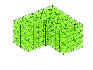
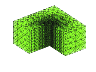
Fig. 1: Coarse mesh(at left) and the second locally refined mesh (at right)

Example 4.2. Consider the eigenvalue problem with $\epsilon=I$ and $\mu=I$ or

$$\mu=\left(\begin{array}[]{ccc}2&1-2j&-j\\ 1+2j&4&j\\ j&-j&5\end{array}\right)$$ (55)

on the thick L-shaped $\Omega=((-1,1)^{2}\backslash(-1,0]^{2})\times(0,1)$. When $\mu=\epsilon=I$ $\lambda_{1}\approx 9.6397$, $\lambda_{2}\approx 11.3452$ and $\lambda_{3}\approx 13.4036$ (see [18]). We use Scheme 3.2 with $i0=1$ to compute the lowest three eigenvalues for both cases. The numerical results are shown in Tables 4.2-4.3. From Table 4.2 we see that the eigenvalue errors obtained by Scheme 3.2 after 2nd iteration are respectively 0.019, 0.012 and 7.0e-04, which indicates the accuracy of the lowest two eigenvalues is affected by the singularity of the associated eigenfunctions in the directions perpendicular to the reentrant edge and the convergence rate $R$ is usually less than 2. Alternately, we adopt the meshes locally refined towards the reentrant edge (see Figure 4.1) to perform the iterative procedure. And the associated numerical results are listed in Table 4.4, which implies the errors of $\lambda^{h_{2}}_{1}$ and $\lambda^{h_{2}}_{2}$ are significantly decreased to 0.0033 and 0.0066 respectively with less degrees of freedom.

Example 4.3. Consider the Maxwell eigenvalue problem with $\Omega=(-\frac{1}{2},\frac{1}{2})\times(0,0.1)\times(-\frac{1}{2},\frac{1}{2})$ where $\mu=I$ and if $x_{3}>0$ then $\epsilon=2I$ otherwise $\epsilon=I$. This is a practical problem in engineering computed in [16, 23]. We use Scheme 3.2 with $i0=1$ to compute the three lowest eigenvalues for both cases. The numerical results are shown in Table 4.5. The relatively accurate eigenvalues reported in [16] are respectively $3.538^{2}(12.5174)$, $5.445^{2}(29.6480)$ and $5.935^{2}(35.2242)$. Using them as the reference values, the relative errors of numerical eigenvalues after 3rd iteration are respectively 6.0877e-05, 3.7524e-05 and 0.0105. Obviously we get the good approximations of the eigenvalues $\lambda_{1}$ and $\lambda_{2}$. Regarding the computation for $\lambda_{3}$, we refer to Table II in [23] whose relative error for computing $\lambda_{3}$ is 0.0107 using a higher order method. This is a computational result very close to ours. Hence we think our method is also efficient for solving the problem.

Example 4.4. Consider the Maxwell eigenvalue problem with $\mu=\epsilon=I$ and $\Omega=(-1,1)^{3}\backslash[-\frac{1}{2},\frac{1}{2}]^{3}$. In this example, we capture a physical zero eigenvalue on a coarse mesh with number of degrees of freedom 6230, i.e., $\lambda_{1,H}=1.9510e-12$. We use Scheme 3.2 with $i0=0$ to compute the eigenvalues $\lambda_{2}$(of multiplicity 3), $\lambda_{5}$(of multiplicity 2) and $\lambda_{7}$(of multiplicity 3). The numerical results are shown in Table 4.6. Note that the coarse mesh seems slightly “fine”. This is because we would like to capture all information of the lowest eight eigenvalues (some of them would not be captured on a very coarse mesh). This is an example of handling the problem in a cavity with two disconnected boundaries. For more numerical examples of the cavity with disconnected boundaries, we refer the readers to the work of [24].

Acknowledgment The author wishes to thank Prof. Yidu Yang for many valuable comments on this paper.

References

- [1] P. Arbenz, R. Geus, and S. Adam, Solving Maxwell eigenvalue problems for accelerating cavities, Phys. Rev. Accelerators and Beams, 4 (2001), 022001.
- [2] P. Arbenz and R. Geus, Multilevel preconditioned iterative eigensolvers for Maxwell eigenvalue problems, Appl. Numer. Math., 54 (2005), pp. 107-121.
- [3] M. Ainsworth, J. Coyle, Computation of Maxwell eigenvalues on curvilinear domains using hp-version Ndlec elements, Numer. Math. Adv. Appl., 2003, pp. 219-231.
- [4] D. Boffi, P. Fernandes, L. Gastaldi, and I. Perugia, Computational models of electromagnetic resonantors: Analysis of edge element approximation, SIAM J. Numer. Anal., 36 (1999), pp. 1264-1290.
- [5] D. Boffi, Fortin operator and discrete compactness for edge elements, Numer. Math., 87 (2000), pp. 229-246.
- [6] D. Boffi, Finite element approximation of eigenvalue problems, Acta. Numerica, 19 (2010), pp. 1-120.
- [7] A. Buffa, P. Ciarlet, and E. Jamelot, Solving electromagnetic eigenvalue problems in polyhedral domains with nodal finite elements, Numer. Math., 113 (2009), pp. 497-518.
- [8] A. Buffa, P. Houston, and I. Perugia, Discontinuous Galerkin computation of the Maxwell eigenvalues on simplicial meshes, J. Comput. Appl. Math., 204 (2007), pp. 317-333.
- [9] F. Brezzi, M. Fortin, Mixed and Hybrid Finite Element Methods, vol. 15, Springer, New York, NY, USA, 1991.
- [10] S. C. Brenner, F. Li , L. Sung, Nonconforming Maxwell Eigensolvers, J. Sci. Comput., 40(2009), pp. 51-85.
- [11] I. Babuska, J. Osborn, Eigenvalue Problems, in: P .G. Ciarlet, J. L. Lions, (Ed.), Finite Element Methods (Part 1), Handbook of Numerical Analysis, vol.2, Elsevier Science Publishers, North-Holand, 1991, pp. 640-787.
- [12] S. Caorsi, P. Fernandes, M. Raffetto, On the Convergence of Galerkin Finite Element Approximations of Electromagnetic Eigenproblems, SIAM J. Numer. Anal., 38(2000), pp. 580-607.
- [13] L. Chen, iFEM: An Integrated Finite Element Methods Package in MATLAB, Technical report, University of California at Irvine, 2009.
- [14] P. Ciarlet, Jr., and G. Hechme, Computing electromagnetic eigenmodes with continuous Galerkin approximations, Comput. Methods Appl. Mech. Engrg., 198 (2008), pp. 358-365.
- [15] J. Chen, Y. Xu, and J. Zou, An adaptive inverse iteration for Maxwell eigenvalue problem based on edge elements, J. Comput. Phys., 229 (2010), pp. 2649-2658.
- [16] A. Chatterjee, J. M. Jin, and J. L Volakis, Computation of cavity resonances using edge based finite elements, IEEE Trans. Microwave Theory Tech., 40 (1992), pp. 2106-2108.
- [17] F. Chatelin, Spectral Approximations of Linear Operators, Academic Press, New York, 1983.
- [18] M. Dauge, Benchmark computations for Maxwell equations for the approximation of highly singular solutions (2004). See Monique Dauge s personal web page at the location http://perso.univ-rennes1.fr/monique.dauge/core/index.html
- [19] V. Girault and P. A. Raviart, Finite Element Methods for Navier-Stokes Equations: Theory and Algorithms, Springer-Verlag, Berlin, 1986.
- [20] R. Hiptmair, Finite elements in computational electromagnetism, Acta Numer., 11 (2002), pp. 237-339.
- [21] R. Hiptmair and J. Xu, Nodal auxiliary space preconditioning in and spaces, SIAM J. Numer. Anal., 45 (2007), pp. 2483-2509.
- [22] X. Hu and X. Cheng, Acceleration of a two-grid method for eigenvalue problems, Math. Comp., 80 (2011), pp. 1287-1301.
- [23] M. M. Ili, B. M. Notaro, Higher order hierarchical curved hexahedral vector finite elements for electromagnetic modeling, IEEE Trans. Microwave Theory Tech., 51(2003), pp. 1026-1033.
- [24] W. Jiang, N. Liu, Y. Yue, Q. Liu, Mixed finite element method for resonant cavity problem with complex geometric topology and anisotropic media, IEEE Trans. Magnetics, 52(2016), 7400108.
- [25] F. Kikuchi, Weak formulations for finite element analysis of an electromagnetic eigenvalue problem, Scientific Papers of the College of Arts and Sciences, University of Tokyo, 38 (1988), pp. 43-67.
- [26] F. Kikuchi, On a discrete compactness property for the Nedelec finite elements, J.fac.sci.univ.tokyo Sect. 1A Math, 36(1989), pp. 479-490.
- [27] A. Kirsch, P. Monk, A finite element method for approximating electromagnetic scattering from a conducting object, Numer. Math., 92(2002), pp. 501-534.
- [28] P. Monk, Finite Element Methods for Maxwell s Equations, Oxford University Press, Oxford, UK, 2003.
- [29] P. Monk, L. Demkowicz, Discrete compactness and the approximation of Maxwell’s equations in , Math. Comp., 70(2000), pp. 507-523.
- [30] J. C. Ndlec, Mixed finite elements in . Numer. Math., 35(1980), pp. 315-341.
- [31] C. J. Reddy, M. D. Deshpande, C. R. Cockrell, F. B. Beck, Finite Element Method for Eigenvalue Problems in Electromagnetics, Nasa Sti/recon Technical Report N, 95(1995).
- [32] A. D. Russo, A. Alonso, Finite element approximation of Maxwell eigenproblems on curved Lipschitz polyhedral domains, Appl. Numer. Math., 59(2009), pp. 1796-1822
- [33] J. Xu, A. Zhou, A two-grid discretization scheme for eigenvalue problems, Math. Comp. 70(1999), pp. 17-25.
- [34] Y. Yang, H. Bi, J. Han, Y. Yu, The Shifted-Inverse Iteration Based on the Multigrid Discretizations for Eigenvalue Problems, SIAM J. Sci. Comput., (37)(2015), pp. A2583-A2606.
- [35] Y. Yang, H. Bi, A two-grid discretization scheme based on shifted-inverse power method, SIAM J. Numer. Anal. 49 (2011), pp. 1602-1624.
- [36] Y. Yang, Y. Zhang, H Bi, Multigrid Discretization and Iterative Algorithm for Mixed Variational Formulation of the Eigenvalue Problem of Electric Field, Abstr. Appl. Anal., 2012(2012), pp. 1-25, doi:10.1155/2012/190768.
- [37] J. Zhou, X. Hu, L. Zhong, S. Shu, L. Chen. Two-Grid Methods for Maxwell Eigenvalue Problem, SIAM J. Numer. Anal., 52(4)(2014), pp. 2027-2047.