Revealing the nonlinear response of a tunneling two-level system ensemble using coupled modes

Abstract

Atomic sized two-level systems (TLSs) in amorphous dielectrics are known as a major source of loss in superconducting devices. In addition, individual TLS are known to induce large frequency shifts due to strong coupling to the devices. However, in the presence of a broad ensemble of TLSs these shifts are symmetrically canceled out and not observed in a typical single-tone spectroscopy experiment. We introduce a two-tone spectroscopy on the normal modes of a pair of coupled superconducting coplanar waveguide resonators to reveal this effect. Together with an appropriate saturation model this enables us to extract the average single-photon Rabi frequency of dominant TLSs to be $\Omega_{0}/2\pi\approx 79$ kHz. At high photon numbers we observe an enhanced frequency shift due to nonlinear kinetic inductance when using the two-tone method and estimate the value of the nonlinear coefficient as $K/2\pi\approx-1\times 10^{-4}$ Hz/photon. Furthermore, the life-time of each resonance can be controlled (increased) by pumping of the other mode as demonstrated both experimentally and theoretically.

The characterization of a nonlinear medium often involves the usage of a strong (pump) field which modifies the medium properties, combined with a weak (probe) field which is used for measurement. When the nonlinear response of a resonant device is probed, the finite linewidth limits the available pumping bandwidth and thus might hide the full nonlinear behavior. Here we show how this problem can be solved by using the normal modes of a coupled system. When two modes share the same spatial volume but have different frequencies, one mode can be pumped strongly, modifying the medium locally overlapping with the other mode which is used for probing. When the splitting between the modes is large enough the pumped mode can modify the spectral components of the medium outside of the other mode’s linewidth. In this Rapid Communication we demonstrate how this method can reveal nonlinear properties which would have remained hidden even for the strongest drive possible if the standard method was used. In particular, we measure low-power nonlinear frequency shifts of resonances formed by coupled superconducting coplanar waveguide resonators (CPWR) Göppl et al. (2008). As we show, these shifts, caused by pumping at a detuning of $\sim 1000$ times the resonance linewidth, are well explained by the saturation of two-level systems (TLSs) in the device’s dielectrics. Thus, this method can be used to give valuable information about TLSs, which was unavailable otherwise. Furthermore, at high powers, when kinetic inductance nonlinearity is dominant, our two-tone method provides twice the nonlinear sensitivity, which might be useful for applications such as microwave kinetic inductance detectors Day et al. (2003) and resonators’ frequency tuning Vissers et al. (2015).

Investigated in the context of amorphous material physics Anderson et al. (1972); Phillips (1972, 1987), TLSs in dielectrics were brought into focus again since the discovery of their critical role as a loss mechanism in superconducting devices Martinis et al. (2005). While the effect of TLSs saturation by probe power on the imaginary part of the dielectric constant $Im\left(\epsilon\right)$ (i.e. internal loss) was investigated thoroughly Von Schickfus and Hunklinger (1977); Martinis et al. (2005); Pappas et al. (2011); Khalil et al. (2011); Sage et al. (2011); Rosen et al. (2016); Skacel et al. (2015), the modification of $Re\left(\epsilon\right)$ (i.e. frequency shift) by the drive has remained hidden Tem . Here we demonstrate how by applying a pump-probe measurement on coupled modes this effect can be revealed.

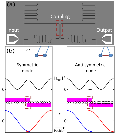
Figure 1: (a) Design of the coupled resonators device Res . Empty area represents Si substrate, gray area represents metal (Al). Feedline and resonators are black for clarity. Dark-red dashed box marks the coupling region. (b) Cartoon of the experimental idea. Magenta bars represent the resonators, the $x$ axis is the position along their lengths. In analogy to coupled pendula the coupling results in the forming of a symmetric and an antisymmetric modes which differ only by the phase between the electric fields in both resonators (blue and red curves) Pen . TLSs (represented by ’X’) experience the same total field intensity (black curves) in both modes, except for the small coupling area in which the resonators’ fields interfere. This allows ignoring other details than the frequency detuning between the modes.

Coupled resonators with a strong Josephson nonlinearity were used e.g. for quantum-limited amplification Eichler et al. (2014), stabilization of photon-number states Holland et al. (2015a) and for simulating a Bose-Hubbard chain Hacohen-Gourgy et al. (2015). Here we use coupled resonators as a tool to characterize the intrinsic nonlinearities of the resonators. For an ideal coupled pair of two identical resonators the normal modes will be a symmetric mode and an antisymmetric one for which the wave functions are identical up to a phase. This allows us to ignore uncertainties e.g. in electric field distribution and treat the modes referring only to the ability to saturate detuned spectral components of the nonlinear medium (see Fig. 1).

Our device consists of two capacitively coupled $\lambda/2$ CPWR made from $\sim 120$ nm Al sputtered on high-resistivity Silicon ($\rho>5000\,\,\Omega\cdot$cm), see Fig. 1. These resonators are physically identical, hence their bare (uncoupled) resonance frequencies are the same, but due to the coupling, two modes split by $\sim 63$ MHz at 5626 and 5689 MHz are formed. We characterize the resonances by measuring the transmission through a common feedline to which they are capacitively coupled using a vector network analyzer. The resonance frequency $f_{0}$, internal quality factor $Q_{i}$ and the steady-state average number of photons $\braket{N}$ stored in the resonator are extracted by fitting the complex transmission data $S_{21}\left(f\right)$ to an appropriate model Khalil et al. (2012); Mazin (2004); Probst et al. (2015); Sup . In order to quantify the nonlinear response of the resonances the probe power is scanned at a range which corresponds to $\langle N\rangle=10^{1}-10^{8}$ photons, and the dependence of various parameters on $\langle N\rangle$ is analyzed. All measurements were conducted at a temperature of $\sim 20$ mK with the device mounted to the base plate of a dilution refrigerator.

In Fig. 2 we show the resonance frequency $f_{0}$ and internal loss $1/Q_{i}$ of the resonances obtained using the standard single-tone spectroscopy method (for a uniform medium and electric field $1/Q_{i}=\tan\delta$, the bulk loss tangent, see Sup ). The frequency of a single-tone probe is scanned around one resonance for various probe powers and the parameters are extracted as detailed above. As shown in Fig. 2b the loss dependence on $\langle N\rangle$ agrees well with the TLS model Sup . In addition, as predicted by this model Pappas et al. (2011), for stored energies corresponding to $\langle N\rangle\lesssim 10^{5}$ there is no observable frequency shift. For higher probe powers there is a strong negative shift which depends linearly on the number of photons. This linear shift is explained as resulting from nonlinear kinetic inductance Zmuidzinas (2012) which can be modeled as a Kerr nonlinearity Yurke and Buks (2006) (the weak negative shift for $10^{5}\lesssim\langle N\rangle\lesssim 10^{7}$ resulting in a discrepancy from the fits at low powers might be due to the finite number of TLSs, see Sup ). We elaborate more on the high power regime below. We stress here that in fact TLSs far detuned from resonance contribute to the real part of the dielectric constant $\epsilon$ Pappas et al. (2011) and therefore should effect $f_{0}$, but because the standard method uses a single tone which saturates TLSs symmetrically around resonance this nonlinear effect is effectively hidden (See Figs. 4a and  4b).

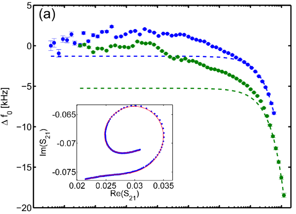
(a)

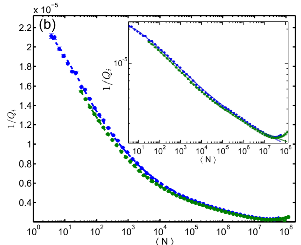
(b)

Figure 2: (a) Resonance frequency shift and (b) Internal loss (shown in a log-log scale in the inset) vs $\langle N\rangle$ for the probe-only experiment for the resonances at 5626 MHz (green) and 5689 MHz (blue). Dashed lines in 2a are linear fits of the high power shifts to a Kerr nonlinearity model as detailed in the text. Dashed lines in 2b are fits to the standard TLS model (Sup Eq. (29)). Inset in Fig. 2a: a typical fit of the transmission data.

The full nonlinear behavior of the resonances is revealed when we use our two-tone pump-probe method. This is done by pumping strongly at a frequency close to one resonance while measuring $S_{21}\left(f\right)$ of the other resonance using a weak probe. Fig. 3a shows the results of this experiment. Notice that while in Fig. 2 the $x$ axis indicates the average number of photons in the probed resonance, in Fig. 3 the $x$ axis shows the average number of photons in the pumped resonance and the weak probe power is held constant Sup . In contrary to the kinetic inductance nonlinearity at high photon numbers which is common to both types of experiments, at lower powers there is a significant frequency shift in the pump-probe experiments which is not observed in the probe-only experiments. Furthermore, the direction of the resonance shift depends on the relative position of the pumped and probed resonances. A negatively-detuned pump induces a negative shift on the probed resonance and vice-versa. These shifts can be explained by generalizing the TLS model to the pump and probe case. We first give a qualitative explanation of the physical reasoning behind the differences and then give the details of the full derivation.

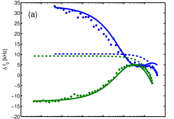
(a)

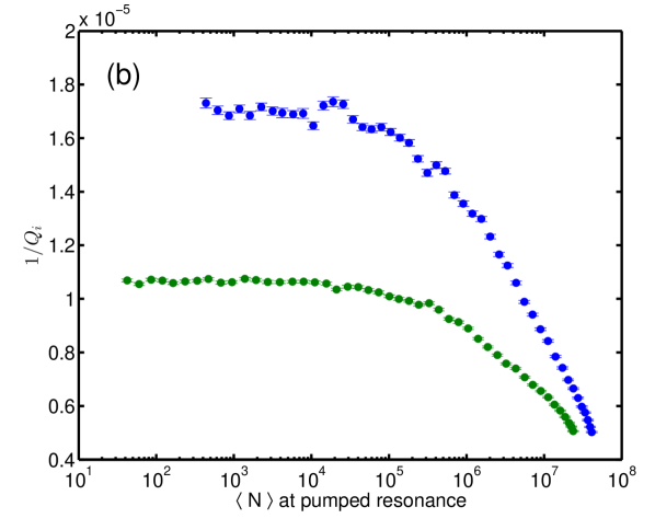
(b)

Figure 3: (a) Resonance frequency shift and (b) Internal loss vs the average number of photons $\langle N\rangle$ in the pumped mode for the pump-probe experiment. Green (blue) points are for probe at 5626 MHz (5689 MHz) and pump at 5689 MHz (5626 MHz). The dashed lines in Fig. 3a are linear fits of the high power shifts to a Kerr nonlinearity model as detailed in the text. Solid lines are sums of the fits to the prediction of the generalized model of frequency shift due to TLSs (Eq. (4)) and the linear fits. In Fig. 3a constant shifts were added for clarity.

Figure 4: Qualitative picture of the generalized TLS saturation model for the resonance shift. A black ’X’ represents a TLS. A red ’X’ represents a saturated TLS. Green arrows represent the level repulsion (the length indicating the repulsion strength). Red arrows represent the pump tone. (a) In the absence of pumping the TLSs are symmetrically distributed around a resonance, resulting in a broadening without a frequency shift. (b) A symmetric pump around one resonance narrows the linewidth without a frequency shift. (c) When two resonances are present, strongly pumping symmetrically around the lower resonance results in an asymmetric repulsion for the higher resonance, causing a frequency shift. (d) When the pump power increases, the repulsion of the higher resonance becomes more and more symmetric, causing a decrease in the frequency shift.

The effect of one TLS on the probed mode frequency can be approximately described by the dispersive shift Blais et al. (2004) $\Delta\omega_{pr}=\frac{g^{2}}{\Delta}\langle\hat{S}_{z}\rangle$, where $g$ is the coupling strength between the TLS and the mode, $\Delta\equiv\omega_{TLS}-\omega_{pr}$ is their detuning and $\hat{S_{z}}=\pm 1$ is a TLS state operator (this result is obtained by applying second order perturbation theory on the Jaynes-Cummings Hamiltonian Jaynes and Cummings (1963), assuming $g<\Delta$ and can be understood as resulting from level repulsion between the mode and the TLS). Since TLSs density of states is uniform in energy Phillips (1987) they will be distributed symmetrically around $\omega_{pr}$ resulting in equal negative and positive shifts which sum to a zero shift with a broadened linewidth (Fig. 4a). When a TLS is pumped strongly it populates the excited state half of the time, yielding $\langle\hat{S_{z}}\rangle=0$. Nevertheless, when the standard probe-only method is used, TLSs are saturated symmetrically around $\omega_{pr}$, hence the effect is only linewidth narrowing (i.e. reducing the internal loss) but no observable frequency shift (Fig. 4b). The situation is different when one mode is pumped while the other is probed. The presence of another mode opens a spectral window for asymmetric saturation of TLSs which effects the probed mode due to the spatial coexistence of both modes’ fields. When a mode negatively (positivity) detuned from the probe field is pumped strongly TLSs negatively (positivity) detuned from $\omega_{pr}$ are saturated, while positivity (negatively) detuned TLSs are less affected, resulting in a negative (positive) net shift (Fig. 4c). Increasing pump power increases also the TLSs saturation (from power broadening), initially increasing the shift but eventually making saturation more and more symmetric, hence reducing the shift (Fig. 4d). We now present a full quantitative model to explain the results Sup . A single TLS is characterized by an asymmetry energy $\Delta_{j}$, a tunneling amplitude $\Delta_{0j}$ resulting in the eigenenergy $E_{j}\equiv\hbar\omega_{j}\equiv\sqrt{\Delta_{j}^{2}+\Delta_{0j}^{2}}$ and an electric dipole moment $p_{j}$ Phillips (1987). The dipole coupling coefficient to a uniform electric field occupying a volume $V$ filled by a material with a dielectric constant $\epsilon$ is $g_{j}\equiv\frac{\cos\theta_{j}p_{j}\sqrt{\omega_{pr}}}{\sqrt{2\hbar\epsilon\epsilon_{0}V}}\frac{\Delta_{0j}}{\hbar\omega_{j}}$, where $\theta_{j}$ is the angle between the electric field and the dipole and $\omega_{pr}$ is the probed mode frequency. Summing contributions from all TLSs we obtain the frequency shift

$$\Delta\omega_{pr}=\mathrm{Re}\left[\sum_{j}g_{j}^{2}\frac{\langle\hat{S}_{z,j}\rangle}{\omega_{j}-\omega_{pr}+\frac{i}{T_{2j}}}\right],$$ (1)

where $T_{2j}=2T_{1j}$ are the relaxation and dephasing times of the TLS (assuming a negligible TLS-TLS interaction). The population difference induced by pumping yields Phillips (1987)

$$\langle\hat{S}_{z,j}\rangle=-\tanh\left(\frac{\hbar\omega}{2k_{B}T}\right)\times$$

$$\left(1-\frac{T_{1j}\Omega_{Rj}^{2}/T_{2j}}{\left(\omega_{j}-\omega_{pump}\right)^{2}+T_{2j}^{-2}\left(1+\Omega_{Rj}^{2}T_{1j}T_{2j}\right)}\right)$$ (2)

where $\omega_{pump}$ is the pump frequency and the TLS Rabi frequency due to pumping is given by

$$\Omega_{Rj}\equiv\frac{\Delta_{0j}}{\hbar\omega_{j}}\cos\theta_{j}\Omega_{0},\,\hbar\Omega_{0}\equiv 2p_{j}F_{pump},$$ (3)

with the pump field $F_{pump}$. Using the standard TLS model distribution we obtain that in the strong field regime $\Omega_{0}T_{1}T_{2}\gg 1$ the frequency shift due to pumping is Sup

$$\frac{\Delta\omega_{pr}}{\omega_{pr}\tanh\left(\frac{\hbar\omega_{pr}}{2k_{B}T}\right)}=\frac{\sqrt{2}P_{0}p^{2}\pi^{2}}{8\epsilon\epsilon_{0}}\frac{\Delta\omega}{\Omega_{0}}\frac{\sqrt{1+\frac{\Omega_{0}^{2}}{2\Delta\omega^{2}}}-1}{\sqrt{1+\frac{\Omega_{0}^{2}}{2\Delta\omega^{2}}}+1},$$ (4)

where $\Delta\omega\equiv\omega_{pump}-\omega_{pr}$ is the detuning between the pump and probe frequencies and $P_{0}$ is the TLSs density of states. As expected from the qualitative picture, for small fields $\left(\Omega_{0}\ll\Delta\omega\right)$ the shift increases with $\langle N\rangle$ as $\Delta\omega_{pr}\propto\Omega_{0}\propto\sqrt{\langle N\rangle}$, while it decreases as $\Delta\omega_{pr}\propto\Omega_{0}^{-1}\propto\langle N\rangle^{-\frac{1}{2}}$ for high fields $\left(\Omega_{0}\gg\Delta\omega\right)$. In addition, the direction of the shift follows the sign of $\Delta\omega$ Sup as expected. In Fig. 3a we show fits to this model for both resonances Sup . From the fits we obtain an estimate to the average single photon Rabi frequency of a dominant TLS $\Omega_{0}^{N=1}/2\pi\approx 79$ kHz Sup . These values confirm the predictions of previous studies Barends et al. (2013); Wenner et al. (2011) and of our Monte-Carlo simulations Sup that TLSs at regions of strong fields dominate the nonlinear behavior. In comparison to the frequency shift the internal loss needs a much larger number of photons to show a significant response (Fig. 3b), This agrees with our theoretical calculations Sup and demonstrates the fact that the imaginary part of $\epsilon$ is only sensitive to nearly resonant TLSs Pappas et al. (2011).

As mentioned above, for large $\langle N\rangle$ a negative frequency shift is observed in both probe-only and pump-probe experiments. This shift can be attributed to nonlinear kinetic inductance Zmuidzinas (2012) which might be explained e.g. as resulting from quasiparticle microwave heating De Visser et al. (2010) or modification of the superconducting ground state by the field Semenov et al. (2016). Following Yurke and Buks Yurke and Buks (2006) we model this effect as a Kerr nonlinearity, resulting in a frequency shift which is linear in the number of photons

$$\Delta f_{0}=\frac{K}{2\pi}\langle N\rangle,$$ (5)

where $K$ is the Kerr coefficient. A linear fit to the single-tone experiments high-power frequency shifts (Fig. 2a) yields $\frac{K}{2\pi}=-1.11(0.05)\times 10^{-4}$ Hz/photon for the resonance at 5626 MHz and $\frac{K}{2\pi}=-1.23\times 10^{-4}$ Hz/photon for the resonance at 5689 MHz. These results agree with order of magnitude estimations based on a simple nonlinear kinetic inductance model Sup . These close values for both resonances agree with the fact that kinetic inductance should depend on the superconducting Al properties Dahm and Scalapino (1997); De Visser et al. (2010); Semenov et al. (2016). Generalizing the model to the case of coupled resonators Sup we find that the expected shift of one resonance due to photons in the other resonance is linear in the number of photons with the coefficient $K^{\prime}=2K$, i.e. doubled. Fitting the two-tone experiments high-power frequency shifts (Fig. 3a) we obtain $\frac{K^{\prime}}{2\pi}=-5(1)\times 10^{-4}$ Hz/photon for the 5626 MHz resonance and $\frac{K^{\prime}}{2\pi}=-2.4(0.8)\times 10^{-4}$ Hz/photon for the 5689 MHz resonance. For the 5689 MHz resonance we obtain an agreement with the expected theoretical doubling, but for the 5626 MHz resonance there is a discrepancy which might be a result of an additional TLS shift due to non-uniform electric field or imperfections in the calculation of the number of photons at high powers Sup . Similar enhancement of the cross-Kerr shift in comparison to the self-Kerr one was observed with a strong Josephson nonlinearity Holland et al. (2015a). Here it is used as a tool for measuring the intrinsic nonlinearity of a presumably linear resonator.

In conclusion, a method for the characterization of nonlinearities using a pump-probe scheme on the normal modes of coupled resonators was implemented and analyzed. Using this method the effect of TLS saturation by drive power on the real part of the dielectric constant $\epsilon$ was uncovered and the average single photon Rabi frequency of dominant TLSs was extracted. In addition, the Kerr coefficient quantifying the strength of nonlinear kinetic inductance was measured, yielding $\frac{K}{2\pi}\approx-1\times 10^{-4}$ Hz/photon. Knowledge of the nonlinearities of presumably linear CPWRs down to the single photon limit is important for quantum information applications, such as the implementation of recent proposals for encoding logical qubits by multiphoton cat states Leghtas et al. (2013). In addition, the ability to reduce the internal loss of one mode by pumping the other mode can be used to enhance the resonance lifetime while keeping the number of probing photons small, as required e.g. for dispersive readout in circuit QED Blais et al. (2004).