Critical level crossings and gapless spin liquid
in the square-lattice spin-$1/2$ $J_{1}$-$J_{2}$ Heisenberg antiferromagnet

Abstract

We use the DMRG method to calculate several energy eigenvalues of the frustrated $S=1/2$ square-lattice $J_{1}$-$J_{2}$ Heisenberg model on $2L\times L$ cylinders with $L\leq 10$. We identify excited-level crossings versus the coupling ratio $g=J_{2}/J_{1}$ and study their drifts with the system size $L$. The lowest singlet-triplet and singlet-quintuplet crossings converge rapidly (with corrections $\propto L^{-2}$) to different $g$ values, and we argue that these correspond to ground-state transitions between the Néel antiferromagnet and a gapless spin liquid, at $g_{c1}\approx 0.46$, and between the spin liquid and a valence-bond-solid at $g_{c2}\approx 0.52$. Previous studies of order parameters were not able to positively discriminate between an extended spin liquid phase and a critical point. We expect level-crossing analysis to be a generically powerful tool in DMRG studies of quantum phase transitions.

The spin-$1/2$ frustrated $J_{1}$-$J_{2}$ Heisenberg model on the two-dimensional (2D) square lattice (where $J_{1}$ and $J_{2}$ are the strengths of the first and second neighbor couplings ${\bf S}_{i}\cdot{\bf S}_{j}$, respectively) has been studied and debated since the early days of the high-$T_{c}$ cuprate superconductors chandra88 ; ed1 ; gelfand89 ; sachdev89 ; ed2 ; singh90 ; RS9173 ; ed3 ; ivanov92 ; ed5 ; ed4 ; Singh_prb60.7278 . The initial interest in the system stemmed from the proposal that frustrated antiferromagnetic (AFM) couplings could lead to a spin liquid (SL) in which preformed pairs (resonating valence bonds fazekas74 ) become superconducting upon doping Anderson (1987); Lee, Nagaosa and Wen (2006). Later, with frustrated quantum magnets emerging in their own right as an active research field diep05 , the $J_{1}$-$J_{2}$ model became a prototypical 2D system for theoretical and computational studies of quantum phase transitions and nonmagnetic states Capriotti_prl84.3173 ; Capriotti_prl87.097201 ; mambrini_prb74.144422 ; sirker_prb73.184420 ; darradi_prb78.214415 ; WangJ1J216 ; arlego_prb78.224415 ; Beach_prb79.224431 ; richter_ed ; HuJ1J2 ; JiangJ1J2 ; ShengJ1J2 ; MurgJ1J2 ; KaoJ1J2 ; WangJ1J2 ; mambrini17 ; HaghshenasJ1J2 . Of primary interest is the transition from the long-range Néel AFM ground state AndersonTower ; chakravarty89 ; manousakis91 at small $g=J_{2}/J_{1}$ to a nonmagnetic state in a window around $g\approx 0.5$ (before a stripe AFM phase at $g\gtrsim 0.6$). The nature of this quantum phase transition has remained enigmatic Singh_prb60.7278 ; Capriotti_prl84.3173 ; sirker_prb73.184420 ; darradi_prb78.214415 ; WangJ1J216 ; mambrini17 , despite a large number of calculations with numerical tools of ever increasing sophistication, e.g., the density matrix renormalization group (DMRG) method whitedmrg ; schollwoechreview ; JiangJ1J2 ; ShengJ1J2 , tensor-product states MurgJ1J2 ; KaoJ1J2 ; WangJ1J2 ; WangJ1J216 ; mambrini17 ; HaghshenasJ1J2 , and variational Monte Carlo HuJ1J2 ; Imada15 .

The nonmagnetic state may be one with spontaneously broken lattice symmetries due to formation of a pattern of singlets (a valence-bond-solid, VBS) or a SL. Within these two classes of potential ground states there are several different proposals, e.g., a columnar RS9173 ; singh90 ; Singh_prb60.7278 versus a plaquette Capriotti_prl84.3173 ; mambrini_prb74.144422 ; ShengJ1J2 ; KaoJ1J2 VBS, and gapless HuJ1J2 or gapped JiangJ1J2 SLs. The quantum phase transition out of the AFM state may possibly be an unconventional ’deconfined’ transition senthil04 ; DQCP2 ; moon12 , which recently has been investigated primarily within other models DQCP3 ; melko08 ; lou09 ; banerjee10 ; block13 ; harada13 ; chen13 ; shao16 ; nahum15 hosting direct AFM–VBS transitions. In the $J_{1}$-$J_{2}$ model, some studies have indicated that the nonmagnetic phase may actually comprise two different phases, with an entire gapless SL phase—not just a critical point—existing between the AFM and VBS states ShengJ1J2 ; Imada15 . However, because of the small system sizes accessible, it was not possible to rule out a direct AFM–VBS transitions. We here demonstrate an intervening gapless SL by locating the AFM–SL and SL-VBS transitions using a numerical level-spectroscopy approach, where finite-size transition points are defined using excited-level crossings. These crossing points exhibit smooth size dependence and can be more reliably extrapolated to infinite size than the order parameters and gaps used in past studies.

We use a variant of the DMRG method whitedmrg ; whiteparadmrg ; McCulloch07 ; schollwoechreview to calculate the ground state energy as well as several of the lowest singlet, triplet and quintuplet excited energies. In the AFM state, the lowest excitation above the singlet ground state in a finite system with an even number of sites is a triplet—the lowest state in the Anderson tower of ’quantum rotor’ states AndersonTower . If the nonmagnetic ground state is a degenerate singlet when the system length $L\to\infty$, as it should be in both a VBS and a topological (gapped) SL, there must be a crossing of the lowest singlet and triplet excitation at a point $g(L)$ that approaches $g_{c}$ with increasing $L$. This is indeed observed at the dimerization transition of the 1D $J_{1}$-$J_{2}$ chain nomura92 ; eggert96 ; sandvik10a and related systems sandvik10b ; suwa_prl15 , and size extrapolations give $g_{c}$ to remarkable precision, even with system sizes only up to $L\approx 30$. A level crossing with the same finite-size behavior was observed recently also in the 2D $J$-$Q$ model suwa_prb94.144416 , which is a Heisenberg model supplemented by four-spin interactions causing an AFM–VBS transition DQCP3 ; melko08 ; lou09 ; banerjee10 ; block13 ; harada13 ; chen13 , likely a deconfined quantum-critical point with unusual scaling properties shao16 . It is then natural to investigate level crossings also in the 2D $J_{1}$-$J_{2}$ model.

We will demonstrate a singlet-triplet level crossing in the $J_{1}$-$J_{2}$ model which for $2L\times L$ cylindrical lattices shifts as $g_{c2}-g_{c2}(L)\propto L^{-2}$ and converges to $g_{c2}\approx 0.52$. We also observe a singlet-quintuplet level crossing, which converges to a different point, $g_{c1}\approx 0.46$. Given the known transitions associated with singlet-triplet crossings, and that a singlet-quintuplet crossing was found at the transition between the critical and AFM states in a Heisenberg chain with long-range interactions sandvik10a ; sandvik10anote , we interpret both $g_{c1}$ and $g_{c2}$ as quantum-critical points. For $g_{c1}\leq g\leq g_{c2}$ the system appears to be a gapless SL with algebraically decaying correlations, as in one of the scenarios proposed in Refs. ShengJ1J2, ; Imada15, (and previously discussed also in Ref. sandvik12, ). Our value of $g_{c1}$ is in the middle of the range $g=0.4\sim 0.5$ where most recent studies have put the end of the AFM phase JiangJ1J2 ; HuJ1J2 ; ShengJ1J2 ; Imada15 , and $g_{c2}$ is close to the VBS-ordering point in Refs. ShengJ1J2, ; Imada15, .

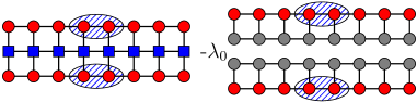
Figure 1: Illustration of the effective Hamiltonian $H_{\text{eff}}^{1}$ below in Eq. (1). Red and gray circles represent the targeted state $|\psi_{1}\rangle$ and the ground state $|\psi_{0}\rangle$, respectively, and the blue squares show the original Hamiltonian as a matrix-product operator. The hatched area represents $U_{1}^{\dagger}|\psi_{1}\rangle$, where $U_{1}$ projects to the canonical MPS for $|\psi_{1}\rangle$ without the hatched area.

DMRG calculations.—The DMRG method whitedmrg is a powerful tool for computing the ground state $|\psi_{0}\rangle$ of a many-body Hamiltonian. By solving a Hamiltonian $H_{\text{eff}}$ in a relevant low-entangled subspace of the full Hilbert space, one can obtain an effective wavefunction, through which the most relevant subspace is selected for the next iteration. A series of such subspace projectors produces the ground state as a matrix product state (MPS), i.e., the wavefunction coefficients are traces of products of local matrices of chosen size $m$ ostlund95 ; schollwoechreview .

The lowest excited state $|\psi_{1}\rangle$ can also be targeted with DMRG McCulloch07 provided that $|\psi_{0}\rangle$ has been pre-calculated. The only difference from a ground-state DMRG algorithm is that one has to maintain the orthogonality condition $\langle\psi_{1}|\psi_{0}\rangle=0$ at each step. Upon reformulating the Hamiltonian for the lowest excited state as $H_{1}=H-\lambda_{0}|\psi_{0}\rangle\langle\psi_{0}|$, where $\lambda_{0}$ is the eigenvalue of $H$ corresponding to $|\psi_{0}\rangle$, one can write down the effective Hamiltonian equation in the DMRG procedure as

$$\left[U_{1}^{\dagger}\left(H-\lambda_{0}|\psi_{0}\rangle\langle\psi_{0}|\right)U_{1}\right]U_{1}^{\dagger}|\psi_{1}\rangle=\lambda_{1}U_{1}^{\dagger}|\psi_{1}\rangle,$$ (1)

where $U_{1}$ projects onto the canonical MPS schollwoechreview for $|\psi_{1}\rangle$ without the center two sites, as illustrated in Fig. 1, and $\lambda_{1}$ is the eigenvalue for $|\psi_{1}\rangle$. We can therefore define an effective Hamiltonian $H^{1}_{\text{eff}}\equiv U_{1}^{\dagger}\left(H-\lambda_{0}|\psi_{0}\rangle\langle\psi_{0}|\right)U_{1}$.

Similarly, given that $|\psi_{i}\rangle$ for all $i<j$ ($\lambda_{i}<\lambda_{j}$) have been pre-calculated, we observe that one can compute the next eigenstate $j$ as an MPS with a given number of kept Schmidt states $m$ using a modified Hamiltonian

$$H_{j}=H-\sum_{i=0}^{j-1}\lambda_{i}|\psi_{i}\rangle\langle\psi_{i}|.$$ (2)

Here $H_{\text{eff}}^{j}U_{j}^{\dagger}|\psi_{j}\rangle=\lambda_{j}U_{j}^{\dagger}|\psi_{j}\rangle$ as in Eq. (1). In practice such a DMRG scheme will break down (i.e., unreasonably large $m$ has to be used) when the eigenstates far from the bottom of the spectrum begin to violate the area law.

The $2L\times L$ cylinder geometry, with open and periodic boundaries in the $x$ and $y$ direction, respectively, is known to be suitable for 2D DMRG calculations white07 and we use it here for even $L$ up to $10$. We employ the DMRG with either U(1) (the total spin $z$ component $S^{z}$ is conserved) or SU(2) symmetry. With $U(1)$ symmetry, we generate up to ten $S^{z}=0$ states and obtain the total spin $S$ by computing the expectation value of ${\bf S}^{2}$.

An advantage of focusing on the level spectrum is the well known fact that the energy converges much faster with the number $m$ of Schmidt states than other physical observables, and also as a function of the number of sweeps in the DMRG procedure. We here apply very stringent convergence criteria and also extrapolate away the remaining finite-$m$ errors based on calculations for several values of $m$ up to $m=12000$ with $U(1)$ symmetry and $m=5000$ with $SU(2)$ symmetry. The DMRG procedures and extrapolations are further discussed in Supplemental Material (SM) sm .

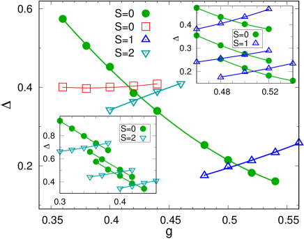
Figure 2: Gaps to the relevant $S=0,1$, and $2$ excitations vs $g$ for $L=10$. The insets show the regions of the level crossings of interest for $L=6,8,10$ (gaps decreasing with increasing $L$). The curves show polynomial fits.

Results.—Figure 2 shows two singlet gaps and the lowest triplet and quintuplet gaps versus $g$ in and close to the non-magnetic regime. The main graph shows results for $L=10$. One of the singlet gaps decreases rapidly with increasing $g$, crossing the other three levels. This is the lowest singlet excitation starting from $g\approx 0.42$, after crossing the other singlet (which has other quantum numbers related to the lattice symmetries) that is lower in what we will argue is the AFM phase. The insets of Fig. 2 show results also for $L=6$ and $8$ in the region around the level crossings that we will analyze (the higher gaps for $L=4$ are not shown for clarity). Using polynomial fits to the DMRG data points, we extract crossing points $g_{c1}(L)$ between the singlet and the quintuplet, as well as $g_{c2}(L)$ between the singlet and the triplet. The singlet-singlet crossings taking place close to $g_{c1}(L)$ are discussed in the SM sm ; their size dependence is similar to $g_{c1}(L)$. For $g\gtrsim g_{c1}(L)$ there are also other levels in the energy range of Fig. 2, including singlets, but the $S=0,1,2$ gaps graphed are the lowest with these spins up to and beyond the largest $g$ shown.

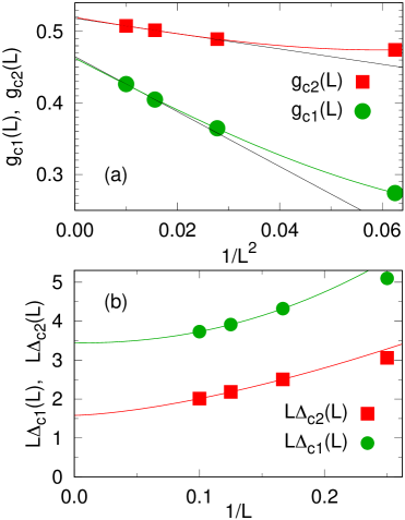
Figure 3: (a) The gap-crossing points from Fig. 2 graphed vs $L^{-2}$. For the singlet-triplet (red squares) and singlet-quintuplet (green circles) data sets, the black lines go through the $L=8,10$ points, while the colored curves are of the form $g_{c}(L)=g_{c}(\infty)+aL^{-2}(1+bL^{-\omega})$ with $g_{c2}(\infty)\approx 0.519$, $g_{c1}(\infty)\approx 0.463$, and $\omega\approx 4$. (b) Size-scaled gaps at the singlet-quintuplet ($\Delta_{c1}$) and singlet-triplet ($\Delta_{c2}$) crossing points along with fits of the form $L\Delta(L)=c+dL^{-\sigma}$, where $\sigma_{1}\approx 2$ and $\sigma_{2}\approx 1.5$.

As $L$ increases the two sets of crossing points drift toward two different asymptotic values. For the singlet-triplet crossings, we have considered different extrapolation procedures with $g_{c2}(L)$, all of which deliver $g_{c2}\approx 0.52$ when $L\to\infty$. It is natural to test whether the finite-size correction to $g_{c2}$ is consistent with the $L^{-2}$ drift in the frustrated Heisenberg chain nomura92 ; eggert96 ; sandvik10a ; a behavior also found in the 2D $J$-$Q$ model in Ref. suwa_prb94.144416, . In Fig. 3(a) we graph the data versus $L^{-2}$ along with a line drawn through the $L=8$ and $L=10$ points, as well as a fitted curve including a higher-order correction. Although we have only four points and there are three free parameters, it is not guaranteed that the fit should match the data as well as it does. With a leading $L^{-1}$ correction the best fit is far from good. Therefore, we take the former fit as evidence that the asymptotic drift is at least very close to $L^{-2}$. The fit with the subleading correction in Fig. 3(a) gives $g_{c2}=0.519$; a minute change from the straight-line extrapolation. Based on the differences between the two extrapolations and roughly estimated errors on the individual crossing points (which arise from the DMRG extrapolations, as discussed in SM sm ), the final result is $g_{c2}=0.519\pm 0.002$.

Plotting the singlet-quintuplet crossing points in the same graph in Fig. 3(a), the overall behavior is similar to the singlet-triplet points, but it is clear that they do not drift as far as to $g_{\rm c2}$. We find that the $L^{-2}$ form applies also here; see the SM sm for further analysis of the corrections for both $g_{c1}$ and $g_{c2}$. A rough extrapolation by a line drawn through the $L=8$ and $L=10$ points gives $g_{\rm c1}\approx 0.465$, and when including a correction, of the same form as in the singlet-triplet case, the extrapolated value moves only slightly down to $g_{\rm c1}\approx 0.463$. Based on this analysis we conclude that $g_{\rm c1}=0.463\pm 0.002$.

In Fig. 3(b) we analyze the crossing gaps, multiplied by $L$ in order to make clearly visible the leading behavior and well-behaved corrections. All gaps close as $L^{-1}$, i.e., the dynamic exponent $z=1$ at both critical points. We have also analyzed the gaps in the regime $g_{\rm c1}<g<g_{\rm c2}$ (not shown), and it appears that the lowest $S=0,1,2$ gaps all scale as $L^{-1}$ throughout. This phase should therefore be a gapless (algebraic) SL, instead of a $Z_{2}$ SL with nonzero triplet gap for $L\to\infty$ JiangJ1J2 and singlet gap vanishing exponentially (due to topological degeneracy).

The point $g_{c2}\approx 0.52$ is higher than almost all previous results reported for the point beyond which the AFM order vanishes, but it is close to where recent works have suggested a transition from a gapless SL into a VBS ShengJ1J2 ; Imada15 . If there indeed is a gapless SL intervening between the AFM and the VBS phases and its lowest excitation is a triplet (as is the case, e.g., in the critical Heisenberg chain), then a singlet-triplet crossing is indeed expected at the SL–VBS transition, since the triplet is gapped and the ground state is degenerate in the VBS phase.

To interpret the singlet-quintuplet crossing at $g_{c1}\approx 0.46$, we again note that the nature of the low-lying gapless excitations reflect the properties of the ground state, and a ground state transition can be accompanied by rearrangements of levels across sectors or within a sector of fixed total spin. A singlet-quintuplet crossing is indeed present at the transition between a critical Heisenberg state (an 1D algebraic SL) and a long-range AFM state in a spin chain with long-range unfrustrated interactions and either unfrustrated laflorencie or frustrated sandvik10a ; sandvik10anote short-range interactions, as we discuss further in the SM sm . This analogy, and the fact that $g_{c1}$ is close to where many previous works have located the end of the AFM phase (as we also show below and in SM sm ), provides compelling evidence for the association of the singlet-quintuplet crossing with the AFM–SL transition. Furthermore, the $S=2$ quantum rotor state in the AFM state has gap $\propto L^{-2}$, while at $g_{c1}$ it scales as $L^{-1}$ according to Fig. 3. Thus, at this point (and for higher $g$) the level spectrum is incompatible with AFM order.

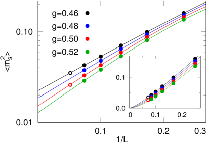
Figure 4: Log-log plot of $\langle m_{s}^{2}\rangle$ vs $L^{-1}$. The curves are of the form $\langle m_{s}^{2}\rangle=bL^{-\alpha}(1-cL^{-\omega})$ with $\omega=0.5$. The leading exponent, with errors estimated by changing $\omega$ within its range of good fits, are $\alpha=1.35\pm 0.05$ ($g=0.46$), $1.53\pm 0.08$ ($g=0.48$), $1.69\pm 0.10$ ($g=0.50$), and $1.78\pm 0.12$ ($g=0.52$). The inset shows the same data on a linear scale. The $L=14$ data (open circles) are from Ref. ShengJ1J2, .

We also computed the squared AFM order parameter (sublattice magnetization per spin) $\langle m^{2}_{s}\rangle$ in the putative SL phase, with ${\bf m}_{s}$ defined on the central $L\times L$ part of the $2L\times L$ system (here with $L$ up to $12$). Since we mainly focused on the excited energies, we did not push the ground state $\langle m^{2}_{s}\rangle$ calculations to as large $L$ as in some past works JiangJ1J2 ; ShengJ1J2 . To complement our own data, we therefore also use $L=14$ results from Ref. ShengJ1J2, . In cases where we have data for the same parameter values, our results agree to within $0.2\%$. We fit the data to power laws with a correction; $\langle m_{s}^{2}\rangle=bL^{-\alpha}(1-cL^{-\omega})$, where acceptable values of $\omega$ span the range $\omega\approx 0.2\sim 1.5$ and the exponent $\alpha$ changes somewhat when varying $\omega$. In Fig. 4 we show examples of fits with $\omega=0.5$. We find that $\alpha$ increases with $g$, from $\alpha\approx 1.3$ at $g=0.46$ to $\alpha\approx 1.8$ at $g=0.52$. We have also tried to fix $\alpha$ to a common value for all $g$, but this does not produce good fits. We therefore agree with previous claims ShengJ1J2 ; Imada15 that the exponent depends on $g$. At $g=0.5$, our result $\alpha\approx 1.7\pm 0.1$ is larger than the value $1.44$ reported in Ref. ShengJ1J2, , with the difference explained by the correction used here. The result agrees well with $\alpha=1.53\pm 0.09$ from variational Monte Carlo calculations Imada15 , and a similar value was also reported with a projected entangled pair state ansatz mambrini17 . In the SM sm we provide further analysis showing that the AFM order vanishes at the extrapolated level crossing point $g_{c1}\approx 0.46$.

Discussion.—Our level-crossing analysis in combination with results for the sublattice magnetization show consistently that the AFM phase ends at $g_{\rm c1}\approx 0.46$ and a gapless SL phase exists between this value and $g_{\rm c2}\approx 0.52$. In the level crossing approach the finite-size transition points are sharply defined and the convergence with system size is rapid, with corrections vanishing as $L^{-2}$ (or possibly $L^{-a}$ with $a\approx 2$). Our results in Fig. 3(a) leave little doubt that the singlet-quintuplet and singlet-triplet crossings converge to different points, while we would expect convergence to the same point if there is no SL between the AFM and VBS phases, as we demonstrate explicitly in the SM sm in the case of the $J$-$Q$ model. The behavior of the spin correlations and the gaps imply a gapless SL with power-law decaying spin correlations. In the region $0.52<g<0.62$, between the SL and the stripe-AFM, our calculations of excited states reveal many low-lying singlets, and we have been able to map them tobeappear onto the expected quasi-degenerate levels expected for a columnar Imada15 VBS state.

The AFM–SL and SL–VBS phase boundaries are in rough agreement with two recent works discussing a gapless SL phase followed by a VBS ShengJ1J2 ; Imada15 , and the lower boundary agrees well with a Lanczos-improved variational Monte Carlo calculation HuJ1J2 . Many other past studies have located the end of the AFM order close to the same value. A recent exception is an infinite-size tensor calculation HaghshenasJ1J2 where the AFM order ends close to our $g_{c2}$ point. However, the infinite-size approach is not unbiased but depends on details of how the environment tensors are constructed. The DMRG calculations, here and in Ref. ShengJ1J2, , are unbiased for finite size if the convergence is checked carefully, and completely exclude AFM order beyond our $g_{c1}$ value.

As far as we are aware, the critical singlet-quintuplet crossing found here (and the singlet-singlet crossing in the SM sm ) has not previously been discussed in the 2D context. This level crossing has been considered in 1D sandvik10a ; sandvik10anote , and in the SM sm we present additional evidence of its association with the AFM–SL transition. The physical origin of the level crossing deserves further study. The detailed information we have obtained on the evolution of the low-energy levels in 2D should be useful for discriminating between different field theoretical descriptions of the phase transitions and the SL phase.

We expect that level crossings are common at 2D quantum phase transitions, as they are in 1D. Our work suggests that the best way to use 2D DMRG in studies of quantum criticality is to first look for and analyze level crossings to extract critical points, and then study order parameters (conventional or topological) at this point and in the phases. In principle the DMRG procedures that we have employed here can also be extended to more detailed level-spectroscopy studies suwa_prb94.144416 ; schuler16 .

Supplemental Material

Critical level crossings in the square-lattice spin-1/2 J1-J2 Heisenberg antiferromagnet

Ling Wang and Anders W. Sandvik

We have argued that the AFM–SL transition in the 2D $J_{1}$-$J_{2}$ Heisenberg model is associated with a level crossing between the lowest singlet excitation and the first quintuplet ($S=2$), while the singlet-triplet crossing is associated with the SL–VBS transition. We here provide further supporting evidence for this scenario.

In Sec. I, we first illustrate our stringent DMRG convergence checks and extrapolations of the low-energy levels. In Sec. II, we contrast the findings for the $J_{1}$-$J_{2}$ model with results for the $J$-$Q$ model, where it is known that no SL phase intervenes between the AFM and VBS states. Accordingly, we show that the singlet-triplet and singlet-quintuplet crossing points flow with increasing system size to the same critical point (a deconfined quantum-critical point). We also investigate the critical scaling of the sublattice magnetization of the $J$-$Q$ model on the cylinders and compare with the $J_{1}$-$J_{2}$ model. In Sec. III we present further tests of the scaling behavior of the level crossing points and the sublattice magnetization of the $J_{1}$-$J_{2}$ model. The singlet-quintuplet crossing in the 2D $J_{1}$-$J_{2}$ model is analogous to a crossing point previously found in a spin chain with long-range interactions at its transition from a critical SL phase to an AFM phase sandvik10a ; sandvik10anote ; laflorencie . In Sec. IV we provide further results for the 1D model, using the excited-level DMRG method to go to larger system sizes than in the past Lanczos calculations. In the 2D $J_{1}$-$J_{2}$ model, in addition to the singlet-quintuplet crossing at the AFM–SL transition, we also find a crossing between the two lowest singlet excitations, and in Sec. V we present the numerical results and analysis of this level crossing.

I. DMRG convergence procedures

In each DMRG calculation bounded by $m$ Schmidt states, we start from a previously converged MPS with a smaller $m$ and perform a number of DMRG sweeps until the energy converges sufficiently. The convergence criterion for an $m$-bounded MPS is that the total energy difference (i.e., not the difference in the average energy per site) between two successive full sweeps is less than $2\times 10^{-6}$, which we have confirmed to be sufficient by comparing with calculations done with less stringent criteria. We then check the convergence of the energies as a function of the discarded weight $\epsilon$ (which depends on $m$, with $\epsilon\to 0$ as $m\to\infty$) defined in the standard way in DMRG calculations as the sum of discarded eigenvalues of the reduced density matrix.

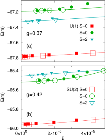
Figure S1: DMRG energies for $L=8$ graphed vs the discarded weight $\epsilon$. The largest number of Schmidt states was $m=2000$ and $m=4000$ for SU(2) and U(1) symmetry, respectively. The curves are fits to constants plus exponential corrections. In both panels, open symbols represent SU(2) energies and the corresponding filled symbols represent U(1) energies; squares for the ground state, circles for the lowest singlet excitation, and triangles for the lowest quintuplet.

In Fig. S1 we show the convergence of the first two $S=0$ energies and the first $S=2$ level for an $L=8$ system at two $g$ values close to $g_{c1}$ (the AFM–SL transition), using $m$ up to $4000$ in calculations with U(1) symmetry and $m$ up to $2000$ with SU(2) symmetry. In our analysis of the AFM-SL transition we used a singlet-quintuplet crossing in the main paper, and in Sec. V we will also investigate the excited singlet-singlet crossing. With SU(2) symmetry implemented, the lowest state in calculations with $S=0$ fixed is the ground state, and we make sure to converge two additional states in this spin sector. At the AFM–SL transition, we further carry out calculations with $S=2$ for the lowest quintuplet. With only U(1) symmetry, the lowest state in the $S^{z}=0$ sector is the ground state, while the lowest state with $S^{z}=2$ is also the lowest excitation with $S=2$. To compute the two lowest singlet excitations close to the AFM–SL transition for $L=8$, one has to go to 6th and 7th excitations in the $S^{z}=0$ sector in the case of $L=8$. In Fig. S1 the SU(2) DMRG eigenvalues nevertheless coincide very well with the corresponding U(1) energies in all cases when $\epsilon$ is small. All the states show exponentially fast convergence when $\epsilon\to 0$, and we can obtain stable extrapolated energies.

For $L=10$, we show the energy convergence at two $g$ values close to $g_{c2}$ (the SL–VBS transition) in Fig. S2, using $m$ up to $12000$ with U(1) symmetry and $m$ up to $5000$ with SU(2) symmetry. The SL–VBS phase transition is detected as the level crossing between the lower singlet and the lowest triplet. With SU(2) symmetry, the lowest state in the $S=0$ sector is the ground state and the lowest triplet is the ground state in the $S=1$ sector. To obtain the lowest singlet excitation used in our analysis in the nonmagnetic state, we target the second $S=0$ state near $g_{c2}$. With U(1) symmetry, the lowest $S^{z}=0$ state is the ground state, while the lowest state in the $S^{z}=1$ sector is the lowest triplet excitation. To compute the first excited singlet for $g_{c1}<g\lesssim g_{c2}$, we need to target the third level with $S^{z}=0$ (since one of the triplet states also has $S^{z}=0$ and is lower in energy than the targeted singlet) but only need the first excitation when $g>g_{c2}$ (since the triplet is higher there). As seen in Fig. S2, for small $\epsilon$ the SU(2) and U(1) energies again coincide very well.

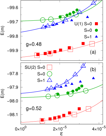
Figure S2: DMRG energies for $L=10$ graphed vs the discarded weight $\epsilon$. The largest number of Schmidt states was $m=5000$ and $m=12000$ for SU(2) and U(1) symmetry, respectively. The curves are fits to constants plus exponential corrections. In both panels, open symbols represent SU(2) energies and the corresponding filled symbols represent U(1) energies: squares for the ground state, circles for the lowest singlet excitation, and triangles for the lowest triplet.

We regard the essentially perfect agreement between the SU(2) and U(1) calculations for large $m$ (in the $L=8$ and $10$ demonstrations above as well as in other cases studied) as evidence for sufficient convergence in both cases. We have estimated the remaining small systematical errors by comparing the U(1) and SU(2) extrapolations in detail and by varying the functional form used in the extrapolations.

II. Critical level crossings and order parameter of the J-Q model on a cylinder

In Ref. suwa_prb94.144416, , the critical level crossings of the lowest singlet and triplet excitation in $J$-$Q$ model were studied using quantum Monte Carlo (QMC) simulations of $L\times L$ lattices with fully periodic (torus) boundaries. The decay rates of the spin-spin and dimer-dimer correlation functions in imaginary time were used to extract the gaps in the triplet and singlet channels, respectively. It was found that the finite size level crossing points $g_{c}(L)$ approach a value $g_{c}$ that is fully consistent with the AFM–VBS quantum critical point previously extracted by finite-size scaling of the order parameters. The scaling correction was found to be $g_{c}(L)-g_{c}\propto L^{-2}$. The level crossing in this case is expected, given the known behaviors of the lowest singlet and triplet in the AFM and VBS states.

In the main text, we concluded that the $J_{1}$-$J_{2}$ model hosts an SL phase between the AFM and VBS states and that the AFM-SL transition is associated with a crossing between $S=0$ and $S=2$ excitations. It is then interesting to look for and investigate singlet-quintuplet level crossings also in the $J$-$Q$ model, as a test that a second, spurious critical point is not found in this case. In addition, it is also useful to study the singlet-triplet crossings with the same DMRG method that we have used for the $J_{1}$-$J_{2}$ model, and with the same cylindrical lattices, to check that we can correctly reproduce the AFM-VBS transition point even in this geometry and with the much more limited system sizes than in the QMC calculations. A related question is whether the change of lattice geometry will affect the power-law scaling behavior of the finite-size size crossing points $g_{c}(L)$.

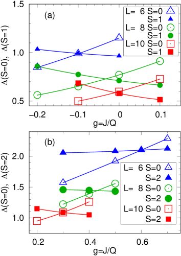
Figure S3: Gaps vs $g=J/Q$ of the $J$-$Q$ model on $2L\times L$ cylinders. (a) The lowest singlet and triplet gaps. (b) The lowest singlet and quintuplet gaps. Both crossing points $g_{c1}(L)$ (singlet-quintuplet) and $g_{c2}(L)$ (singlet-triplet) are extracted using second-order polynomial fits (the curves shown).

We study the lowest singlet-triplet and singlet-quintuplet gap crossings in the standard $J$-$Q$ model DQCP3 , using the DMRG method with U(1) symmetry on $2L\times L$ cylinders with $L=4,6,8,10$. Before presenting the DMRG results, we recall some of the well studied ground state properties of the model from previous QMC simulation in both the torus and cylinder geometries  DQCP3 ; sandvik12 . At $Q=0$, the $J$-$Q$ model reduces to the standard 2D Heisenberg model with AFM order, while at $J=0$ the ground state is a columnar VBS with four-fold degeneracy on a torus. When tuning the coupling ratio $g\equiv J/Q$ from $+\infty$ to $0$, the system goes through a deconfined quantum phase transition from the AFM phase to the columnar VBS phase at $g_{c}\approx 0.045$, where the lowest singlet and triplet gaps cross each other when $L\to\infty$ as mentioned above. In addition, it is known that the ground state of the $J$-$Q$ model on $2L\times L$ cylinders in the VBS phase is a non-degenerate columnar VBS state with $x$-oriented dimers. In our DMRG calculations presented below, we resolve that, in the VBS phase, the ground state has momentum $k_{y}=0$, and above it there is a singlet excited state with momentum $k_{y}=\pi$. The $k_{y}=\pi$ singlet, which is related to the open $x$-direction boundary condition, lies below the first triplet excitation and remains with a non-vanishing gap to the unique ground state in the thermodynamic limit.

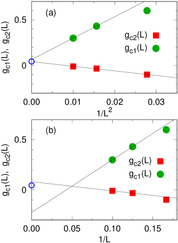
Figure S4: Size dependence of the singlet-triplet (red squares) and singlet-quintuplet (green circles) gap crossing points extracted from the data in Fig. S3. (a) The crossing points graphed vs $L^{-2}$. The lines are drawn through the $L=8$ and $L=10$ points and give the extrapolated crossing values $g_{c2}(\infty)\approx 0.043$ and $g_{c1}(\infty)\approx 0.066$. Both these fall close to the known AFM–VBS transition of the $J$-$Q$ model; $g_{c}=0.045$ (indicated by the blue circle). (b) The crossing points graphed vs $L^{-1}$, with lines drawn through the $L=8$ and $L=10$ points. Here the extrapolated crossing points deviate significantly from the critical point.

Figure S3 shows the gaps versus $g$ on $2L\times L$ cylinders with $L=6,8,10$, with singlets and triplets analyzed in (a), and the singlets and quintuplets in (b). We fit second order polynomials to the data and interpolate for the crossing points. As $L$ increases, the singlet-triplet crossing points $g_{c2}(L)$ drift toward $g_{c}$ from the left, while the singlet-quintuplet crossing points $g_{c1}(L)$ drift toward $g_{c}$ from the right.

It is again natural to check whether the finite-size corrections to the crossing points $g_{c}$ is consistent with the same form, $L^{-2}$, as in the model on a torus. Fig. S4(a) shows $g_{c1}(L)$ and $g_{c2}(L)$ versus $L^{-2}$ along with a line drawn through the $L=8,10$ points. These simple extrapolations give $g_{c2}=0.043$ (singlet-triplet) and $g_{c1}=0.066$ (singlet-quintuplet). Considering the small systems and the extrapolation without any corrections, these results are both in reasonable agreement with the known critical point, $g_{c}\approx 0.045$. The results also support leading $L^{-2}$ corrections for the cylindrical lattices and lend further credence to our use of this form of the corrections in the $J_{1}$-$J_{2}$ model. In contrast, if we assume that the crossing points drift as $L^{-1}$, as shown in Fig. S4(b), the extrapolated points $g_{c2}$ and $g_{c1}$ are very different and disagree with the known critical coupling.

We analyze the gaps $\Delta_{c1}(L)$ and $\Delta_{c2}(L)$ of the $J$-$Q$ model at the $L$-dependent crossing points in Fig. S5. We have multiplied the gaps by $L$ and graph the results versus $L^{-1}$. We see clear signs of convergence to constants, confirming that the gaps close as $L^{-1}$ at the critical point, as expected since the dynamic critical exponent is $z=1$.

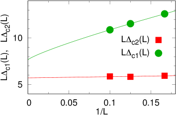
Figure S5: Size-scaled gaps of the $J$-$Q$ model at the size dependent singlet-quintuplet ($\Delta_{c1}$) and singlet-triplet ($\Delta_{c2}$) crossing points from Fig. S3. The curves are fits with power-law corrections to the infinite-size values.

Next, we consider the AFM order parameter of the $J$-$Q$ model, the squared staggered magnetization. Fig. S6 shows $\langle m_{s}^{2}\rangle$ computed in the center $L\times L$ section of $2L\times L$ cylinders at various coupling ratios $J/Q$. The results are graphed versus $L^{-1}$ on log-log scales, along with the results for the same quantity (defined in the same way on the central parts of the cylinders) for $J_{1}$-$J_{2}$ model at $J_{2}/J_{1}=0.5$. Here the results for the $J$-$Q$ model are obtained from QMC simulation (with the same cylindrical boundary conditions that we use in the DMRG calculations), in order to reach the same system sizes as for the $J_{1}$-$J_{2}$ model. The red line on the log-log plot corresponds to a power-law form of $\langle m^{2}_{s}\rangle$ at $g_{c}$. Away from $g_{c}$, inside the AFM phase, we observe that $\langle m^{2}_{s}\rangle$ curves upward for the larger sizes relative to the critical power law behavior, as expected when the order parameter scales to a non-zero value. This is in contrast to the behavior in the case of the $J_{1}$-$J_{2}$ model at $J_{2}/J_{1}=0.5$, where $\langle m^{2}_{s}\rangle$ decays almost in the same way as in the critical $J$-$Q$ model, though on close examination one can see a clear downward trend with increasing size. It therefore appears very unlikely that a non-zero value would survive in the $J_{1}$-$J_{2}$ model when $L\to\infty$; thus the results lend further support to the SL scenario.

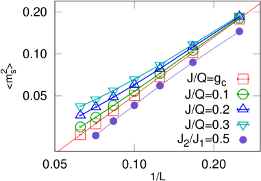
Figure S6: Log-log plot of $\langle m_{s}^{2}\rangle$ of the $J$-$Q$ model vs $L^{-1}$. The results were computed in the central $L\times L$ square of $2L\times L$ cylinders. The red line is a linear fit (power-law scaling) at $g=0.0447\approx g_{c}$. Filled circles are for the same quantity in the $J_{1}$-$J_{2}$ model at $J_{2}/J_{1}=0.5$ (our own DMRG results for $L\leq 12$ and the $L=14$ point from from Ref. ShengJ1J2, ).

III. Additional tests of scaling in the $J_{1}$-$J_{2}$ model

In the main text we showed that leading $L^{-2}$ corrections also describe well the drifts of crossing points in the case of the $J_{1}$-$J_{2}$ model. In Fig. S7(a) we again show the results for $L=6,8,10$ (leaving out $L=4$ for clarity) graphed against $L^{-2}$ together with a simple fit based on just the two largest system sizes. Figure S7(b) shows the same data plotted versus $L^{-1}$, again along with extrapolations using only the two largest system sizes. Since the overall size dependence of the singlet-triplet crossing is weak, its extrapolation only changes marginally from the one based on the $L^{-2}$ form. An extrapolation with a higher-order correction (not shown in the figure) shifts the value down even closer to the previous estimate. The $L^{-1}$ extrapolated singlet-quintuplet point is significantly higher then previously, but looking at the trend including the smaller sizes makes it clear that higher-order fits here will also reduce the extrapolated value. As mentioned in the main text, such higher-order fits do not match the data as well as in the case of leading $L^{-2}$ corrections.

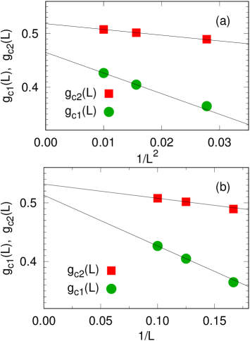
Figure S7: (a) The crossing points of the $J_{1}$-$J_{2}$ model on lattice sizes $L=6,8$, and $10$ (from Fig. 2 in the main paper) graphed vs $L^{-2}$ with leading-order extrapolations with the $L=8$ and $L=10$ data. (b) The same data graphed vs $L^{-1}$ together with leading-order linear fits.

These results with different fitting forms lend support to the existence of a gap between the extrapolated $g_{c1}$ and $g_{c2}$ values in the $J_{1}$-$J_{2}$ and the absence of such a gap in the $J$-$Q$ model. In the main text we have argued that $g_{c1}\not=g_{c2}$ reflects the presence of an SL phase intervening between the AFM and VBS phases in the $J_{1}$-$J_{2}$ model, while $g_{c1}=g_{c2}$ reflects the known deconfined quantum-critical AFM–VBS point in the $J$-$Q$ model. The well established $L^{-2}$ scaling in the latter case, from large-scale QMC simulations suwa_prb94.144416 as well as the results in Sec. II above, allow us to make a further argument against the deconfined quantum-criticality scenario in the $J_{1}$-$J_{2}$ model: If the two models both host critical AFM–VBS points, based on the deconfined universality class, they should also both exhibit leading $L^{-2}$ drifts of the crossing points and common extrapolated crossing points $g_{c1}=g_{c2}$. However, the results shown in Fig. S7(a) and Fig. 3 in the main paper are inconsistent with a common crossing point, unless the system sizes we have access to here are not yet in the asymptotic regime where scaling with small corrections is applicable. While we cannot in principle exclude that a cross-over to a single point, a direct AFM–VBS transition, occurs on some larger length scale, we see no a priori physical reason for such large finite-size effects (given their absence in the $J$-$Q$ model) and find this scenario unlikely. Thus, based on all the present evidence we conclude that the deconfined critical point most likely is expanded into a stable nonmagnetic phase in the $J_{1}$-$J_{2}$ model.

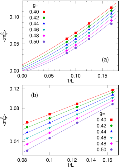
Figure S8: (a) Squared sublattice magnetization of the $J_{1}$-$J_{2}$ model graphed vs $L^{-1}$. The curves are second order polynomials fitted to the $L=8,10,12$ data. (b) Log-log plot of the same data. Here the lines have been fitted to the $L=6,8,10$ points, to illustrate the upward curvature for larger sizes (here $L=12$) in the AFM ordered regime $g<0.46$.

In Fig. 4 of the main paper we analyzed the sublattice magnetization of the $J_{1}$-$J_{2}$ model inside the putative SL phase and found power-law behaviors in the inverse system size. Here we present additional results and analysis both below and above the crossing points $g_{c1}\approx 0.46$, demonstrating the existence of long-range AFM order for $g<g_{c1}$ and the absence of order for $g>g_{c1}$. Fig. S8(a) shows results graphed versus $L^{-1}$ together with second-order polynomial fitted to the data for $L=8,10,12$, representing the expected asymptotic $L^{-1}$ form in the AFM state and a likewise expected $L^{-2}$ next correction. The curves extrapolate to clearly positive values for $g=0.40,0.42$, and $0.44$, while the value at $g=0.46$ is almost zero. For larger $g$ the extrapolated values are negative, indicating that the functional form used is incorrect. One should expect the neglected higher-order corrections to also influence the extrapolated values for smaller $g$, and the deviations between the fitted curve and data at $L=6$ give some indication of the size of the extrapolation errors for $g=0.40-0.46$. The results are consistent with the long-range order vanishing at $g\approx 0.46$, in excellent agreement with the result $g_{c1}\approx 0.46$ obtained from the singlet-quintuplet crossing points. Cubic fits (not shown) to the $L\geq 6$ data result in slightly larger extrapolated values of $\langle m_{s}^{2}\rangle$, but the $g$ dependence is less smooth than with the quadratic fits (likely reflecting sensitivity to the small numerical errors in the individual data points and neglected corrections of still higher order). For $g\geq 0.46$ the cubic polynomials produce negative extrapolated values, supporting the conclusion drawn from the quadratic extrapolations that the AFM order vanishes close to $g=0.46$.

Further support for a critical AFM point at $g\approx 0.46$ is provided in Fig. S8(b). Here we show the data on log-log scales, with straight lines (corresponding to power laws) drawn through the $L=6,8,10$ data. For $g=0.40,0.42$, and $0.44$, the $L=12$ points fall above the lines, reflecting an upward curvature as $L$ increases and AFM order is established. The behavior is similar to that of the $J$-$Q$ model in the AFM phase close to the critical point, e.g., at $J/Q=0.1$ in Fig. S6. For $g=0.46$, all four data points follow the fitted line very closely, while for larger $g$ the $L=12$ points fall below the fitted lines, reflecting negative curvature. In Fig. 4 of the main paper we fitted the data in the putative SL phase to a power law with an additional correction of higher power, required in order to fit all the available data for $g>0.46$.

Overall, these results and those in the main paper support a scenario of a critical AFM–SL point at $g_{c1}\approx 0.46$ at which the scaling corrections are small, while for larger $g$ inside the SL phase the exponent of the asymptotic power law changes and corrections are needed to explain the data on the relatively small systems accessible in DMRG calculations.

IV. Spin chains with long range interactions

The spin-$1/2$ $J_{1}$-$J_{2}$ Heisenberg chain is a celebrated example of a system hosting a quantum phase transition between quasi-long-range ordered (QLRO) and ordered VBS phases. Defining $g=J_{2}/J_{1}$, the transition is located at $g_{c}\approx 0.2411$ nomura92 and is accompanied by a critical level crossing of the lowest singlet and triplet excitations. To study a quantum phase transition between a 1D long-range AFM ordered and QLRO ground states, Laflorencie et al. proposed laflorencie a Heisenberg chain with long-range interactions, with Hamiltonian

$$H=\sum_{i=1}^{L}[\mathbf{S}_{i}\cdot\mathbf{S}_{i+1}+\lambda\sum_{r=2}^{L/2}J_{r}\mathbf{S}_{i}\cdot\mathbf{S}_{i+r}].$$ (S1)

where the couplings are of the form

$$J_{r}=\frac{(-1)^{r-1}}{r^{\alpha}},$$ (S2)

and $\alpha$ and $\lambda$ are both adjustable parameters. Later on, to look for a possible 1D quantum phase transition between AFM and VBS phases, a modification of the model was introduced in which the second neighbor coupling $J_{2}$ changes sign, making it a frustrated term sandvik10a ;

$$H=\sum_{i=1}^{L}\sum_{r=1}^{L/2}J_{r}\mathbf{S}_{i}\cdot\mathbf{S}_{i+r},$$ (S3)

where the couplings are given by

$$J_{2}=g,\quad J_{r\neq 2}=\frac{(-1)^{r-1}}{r^{\alpha}}\left(1+\sum_{r=3}^{L/2}\frac{1}{r^{\alpha}}\right)^{-1},$$ (S4)

where the adjustable parameters are $\alpha$ and $g$ and the normalization of $J_{r\not=2}$ is chosen such that the sum of all nonfrustrated ($r\not=2$) interactions $|J_{r}|$ equals $1$.

For the unfrustrated chain, a curve of continuous AFM–QLRO transitions was mapped out in the $(\alpha,\lambda)$ plane laflorencie . In the frustrated chain, it was found that, by fixing the frustration strength $g$ and tuning the exponent $\alpha$ controlling the long-range interaction, two quantum phase transitions take place along this path sandvik10a ; a QLRO-VBS transition with singlet-triplet excitation level crossing as in the $J_{1}$-$J_{2}$ chain, and, for smaller $\alpha$, an AFM-QLRO transition accompanied by another level crossing. This second crossing was claimed to be a singlet-singlet crossing, but it turns out that (as found in the course of the work reported here) that the total spin $S$ of one of the levels was misidentified as a singlet though it actually is an $S=2$ quintuplet and the crossing discussed is a singlet-quintuplet crossing. In other respects we fully agree with the previous results. Thus, the behavior of the frustrated long-range interacting chain upon increasing $\alpha$ is very similar to that we have observed in the square-lattice $J_{1}$-$J_{2}$ model upon increasing $g=J_{2}/J_{1}$.

In the case of the unfrustrated model with $J_{r}$ given by Eqs. (S2) we also expect the AFM-QLRO quantum phase transition to be accompanied by a singlet-quintuplet excitation crossing, though level crossings were not discussed in Ref. laflorencie, . Here we revisit the quantum phase transitions in both the frustrated and unfrustrated chain models, analyzing level crossings obtained by the SU(2) DMRG method to push to large system sizes than what was possible with the previous Lanczos calculations in Ref. sandvik10a, . This will provide us with further, indisputable evidence that the AFM–QLRO transition in the 1D system indeed is accompanied with a singlet-quintuplet crossing. This in turn gives added credence to our claim of this scenario for the 2D $J_{1}$-$J_{2}$ model.

In the unfrustrated model we set $\lambda=1$ in Eq. (S1) and study the AFM-QLRO quantum phase transition by tuning the long-range interaction exponent $\alpha^{-1}$. In the frustrated model, Eq. (S3), we choose a path with fixed $g=0.3$ in Eq. (S4) and vary $\alpha^{-1}$ from $1$ to $0$, thus passing through both the AFM–QLRO and QLRO–VBS transitions.

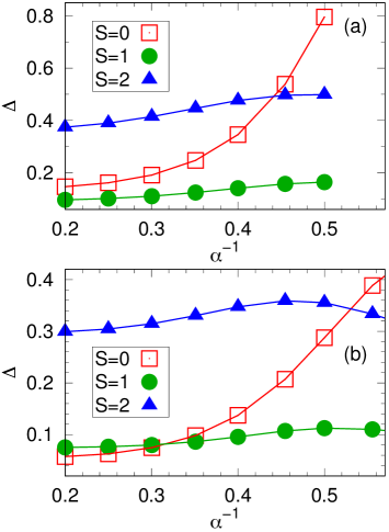
Figure S9: The lowest excitation gaps in singlet ($S=0$), triplet ($S=1$) and quintuplet ($S=2$) sectors in (a) the unfrustrated spin chain with long range interactions and in (b) the frustrated spin chain with long range interactions, both for chain length $L=48$. The gaps are graphed vs the exponent $\alpha^{-1}$ controlling the decay of the long-range interaction with (a) $\lambda=1$ in Eq. (S1) and (b) $g=0.3$ in Eq. (S4). Solid lines are guides to the eye.

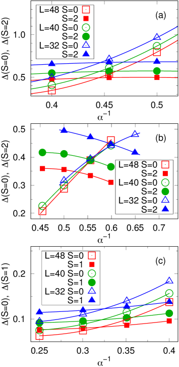
Figure S10: Gaps vs $\alpha^{-1}$ in (a) the unfrustrated spin chain with long-range interactions at $\lambda=1$ in Eq. (S1) and (b-c) the frustrated spin chain with long range interactions at $g=0.3$ in Eq. (S4). All three crossing points $g_{c}(L)$ (singlet-quintuplet, unfrustrated model), $g_{c1}(L)$ (singlet-quintuplet, frustrated model) and $g_{c2}(L)$ (singlet-triplet, frustrated model) are extracted using second-order polynomial fits (the curves shown).

In Fig. S9 we plot the lowest singlet, triplet and quintuplet gaps of $L=48$ chains versus $\alpha^{-1}$ at (a) fixed $\lambda=1$ in the unfrustrated model and (b) fixed $g=0.3$ in the frustrated chain. In both models, the crossing points of the lowest singlet-quintuplet excitations indicate the AFM-QLRO quantum phase transitions, based on the behaviors previously found for the sublattice magnetization. In the frustrated case, the crossing of the lowest singlet and triplet excitations marks the QLRO-VBS quantum phase transition, in analogy with the case of the conventional $J_{1}$-$J_{2}$ Heisenberg chain without the $J_{r>2}$ (which also corresponds to $\alpha=\infty$ in the long-range model).

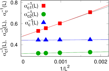
Figure S11: The gap-crossing points in Fig. S10 graphed vs $L^{-2}$. The singlet-quintuplet crossing points in the unfrustrated case are shown as blue triangles, the singlet-quintuplet points in the frustrated case as red squares, and the singlet-triplet point in the frustrated case as green circles. The black lines are drawn through the $L=40$ and $48$ points, while the corresponding colored curves are of the form $\alpha^{-1}_{c}(L)=\alpha^{-1}_{c}(\infty)+aL^{-2}(1+bL^{-\omega})$ with $\alpha^{-1}_{c}(\infty)\approx 0.4434$, $\alpha^{-1}_{c1}(\infty)\approx 0.476$, and $\alpha^{-1}_{c2}(\infty)\approx 0.316$.

We further examine the drifts of these critical level crossings for different system sizes, $L=32,40,48$, in the critical regions. In Fig. S10 the gaps are fitted to second order polynomials to interpolate the finite-size critical points $\alpha^{-1}_{c}(L)$ (singlet-quintuplet in the unfrustrated case), $\alpha^{-1}_{c1}(L)$ (singlet-quintuplet in the frustrated case), and $\alpha^{-1}_{c2}(L)$ (singlet-triplet in the frustrated case). Fig. S11 shows the size dependence of all these crossing points versus $L^{-2}$ along with lines drawn through the data for the largest two sizes, $L=40$ and $48$. We also show fitted curves including a higher-order correction, which give the infinite-size extrapolated values $\alpha^{-1}_{c}=0.4434$, $\alpha^{-1}_{c1}=0.476$, and $\alpha^{-1}_{c2}=0.316$. In the unfrustrated model, the critical value $\alpha^{-1}_{c}=0.4434$, i.e., $\alpha_{c}=2.255$, is fully consistent with the quantum critical point $\alpha_{c}=2.225\pm 0.025$ found by analyzing QMC results for the AFM order parameter in Ref. laflorencie . Thus, there is no doubt that the singlet-quintuplet crossing really marks the AFM–QLRO transition in the unfrustrated chain and there is no reason why this should not be the case also in the frustrated model; indeed the behavior of the order parameters (not shown here) also supports the existence of the phase transition.

V. Singlet-singlet level crossing

As seen in Fig. 2 in the main paper, there is also a singlet-singlet level crossing in the neighborhood of the singlet-quintuplet point analyzed in the main paper. We call the singlet-singlet crossing point $g_{c1}^{\prime}(L)$ and investigate its behavior here.

In Fig. S12(a) we demonstrate the singlet-singlet level crossing for different system sizes and study the trend of this crossing point as a function of the inverse system size in Fig. S12(b). A plausible $L^{-2}$ correction is again assumed here. Then a rough extrapolation to infinite size by a line drawn through the $L=8$ and $L=10$ points in the figure gives $g^{\prime}_{c1}\approx 0.454$. On including a correction with the same fitting form as in the singlet-triplet case, the extrapolated value moves slightly down to $g^{\prime}_{c1}=0.453$. This value is very close to $g_{c1}=0.463$, marking the AFM-SL ground states phase transition as given by the singlet-quintuplet crossing point. Thus, it seems plausible that the AFM-SL transition is associated with both singlet-singlet and singlet-quintuplet excitation crossings, though larger system sizes would be needed to confirm whether the points really flow to the same values.

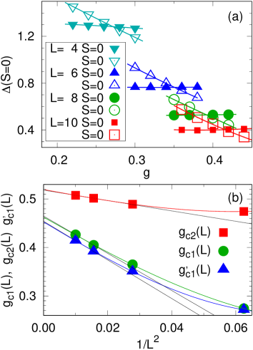
Figure S12: (a) The singlet gaps graphed in Fig. 2 in the main paper for system sizes $L=4,6,8,10$ in the neighborhood of the points at which the two levels cross each other. The crossing points are extracted using second-order polynomial fits. (b) The singlet-singlet crossing points in (a) graphed vs $L^{-2}$ (blue triangles), together with the singlet-quintuplet crossing points (green circles) and singlet-triplet crossing points (red squares). The black line following the blue triangles is drawn through the $L=8,10$ points, while the blue curve is of the form $g_{c}(L)=g_{c}(\infty)+aL^{-2}(1+bL^{-\omega})$ with $g^{\prime}_{c1}(\infty)\approx 0.453$, and $\omega^{\prime}_{1}\approx 3.7$ for fitting the singlet-singlet crossing points.

It should be noted that we have not found any singlet-singlet crossing at the AFM–QLRO transition in the case of the 1D chain discussed above in Sec. III. The singlet-quadruplet crossing point along with its scaling in energy as $L^{-1}$, shown in Fig. 3(b) of the main paper, is also a more clear-cut indicator of a transition out of the AFM state in the sense that we know that the $S=2$ level is a quantum-rotor state that scales as $L^{-2}$ in the AFM state. In principle, the singlet-singlet crossing could be accidental and unrelated to the AFM–SL transition, though the close proximity to the singlet-quadruplet crossing in our extrapolations based on rather small sizes would suggest that it actually is also associated with the transition in the 2D model.