Isostatic equilibrium in spherical coordinates and implications for crustal thickness on the Moon, Mars, Enceladus, and elsewhere

Abstract

Isostatic equilibrium is commonly defined as the state achieved when there are no lateral gradients in hydrostatic pressure, and thus no lateral flow, at depth within the lower viscosity mantle that underlies a planetary body’s outer crust. In a constant-gravity Cartesian framework, this definition is equivalent to the requirement that columns of equal width contain equal masses. Here we show, however, that this equivalence breaks down when the spherical geometry of the problem is taken into account. Imposing the “equal masses” requirement in a spherical geometry, as is commonly done in the literature, leads to significant lateral pressure gradients along internal equipotential surfaces, and thus corresponds to a state of disequilibrium. Compared with the “equal pressures” model we present here, the “equal masses” model always overestimates the compensation depth—by $\sim$27% in the case of the lunar highlands and by nearly a factor of two in the case of Enceladus.

Gindraft=false HEMINGWAY & MATSUYAMA ISOSTASY ON A SPHERE Corresponding author: D. J. Hemingway, Department of Earth and Planetary Science, University of California, Berkeley, 94720, USA. (djheming@berkeley.edu)

1 Introduction

Rocky and icy bodies with radii larger than roughly $200\,\mathrm{km}$ typically have figures that are close to the expectation for hydrostatic equilibrium (i.e., the surface conforms roughly to a gravitational equipotential) because their interiors are weak enough that they behave like fluids on geologic timescales. Because of high effective viscosities in their cold exteriors, however, these bodies can maintain some non-hydrostatic topography, even on long timescales. This non-hydrostatic topography may be supported in part by bending and membrane stresses in the lithosphere [e.g., Turcotte et al., 1981], but over long timescales, and especially when considering broad topographic loads, or loads that formed at a time when the lithosphere was weak, the rocks may yield until much of the support comes from buoyancy—that is, the crustal material essentially floats on the higher density, lower viscosity mantle material beneath it. This is the classic picture of isostatic equilibrium, first discussed by Pratt and Airy in the 1850s, and is often invoked as a natural mechanism by which gravity anomalies associated with topography can be compensated [e.g., Heiskanen and Vening-Meinesz, 1958; Watts, 2001]. The two standard end-member models for isostatic compensation are Airy, involving lateral variations in crustal thickness, and Pratt, involving lateral variations in crustal density.

The problem of modeling Airy-type isostatic compensation can be framed as the need to compute the deflection of the interface between the crust and the underlying higher density, lower viscosity material (we address Pratt-type compensation in the Supporting Information, section S2). Given the known surface topography ($h_{t}$), the Airy-compensated basal topography ($h_{b}$) can be computed as

$$h_{b}=-h_{t}\frac{\rho_{c}}{\Delta\rho}$$ (1)

where $\rho_{c}$ is the density of the crustal material and $\Delta\rho$ is the density contrast at the crust/mantle interface. The negative sign reflects the fact that the basal topography is inverted with respect to the surface topography if both $h_{t}$ and $h_{b}$ are taken as positive upward relief with respect to their respective reference levels (i.e., the hypothetical equipotential surfaces to which the density interfaces would conform if the layers were all inviscid). This equation follows from requiring equal hydrostatic pressures at equal depths (or equivalently, requiring equal masses in columns of equal width), and ensures that, regardless of the topography, there are no horizontal pressure gradients and thus there is no lateral flow at depth within the fluid mantle (there is also no vertical flow because vertical pressure gradients are balanced by gravity). Hence—neglecting mantle dynamics and the slow relaxation of the crust itself—we have a state of equilibrium.

Equation (1) implicitly assumes a Cartesian geometry and a uniform gravity field. However, for long wavelength loads or when the compensation depth is a substantial fraction of the body’s radius, it becomes necessary to take into account the spherical geometry of the problem. In this case, the requirement of equal masses in equal width columns leads to (section 2.2)

$$h_{b}=-h_{t}\frac{\rho_{c}}{\Delta\rho}\left(\frac{R_{t}}{R_{b}}\right)^{2}$$ (2)

where $R_{t}$ and $R_{b}$ are the mean radii corresponding to the top and bottom of the crust, respectively. This expression (or its equivalent) is widely used in the literature [e.g., Jeffreys, 1976; Phillips and Lambeck, 1980; Hager, 1983; Lambeck, 1988; Wieczorek and Phillips, 1997; Wieczorek and Zuber, 2004; Hemingway et al., 2013; McKinnon, 2015; Wieczorek, 2015; Čadek et al., 2016, 2017]. However, as we show in section 2.3, this is not equivalent to the requirement of equal pressures at equal depths, which instead leads to

$$h_{b}=-h_{t}\frac{\rho_{c}}{\Delta\rho}\left(\frac{g_{t}}{g_{b}}\right)$$ (3)

where $g_{t}$ and $g_{b}$ are the mean gravitational accelerations at the top and bottom of the crust, respectively. Although the distinction between “equal masses” and “equal pressures” isostasy has long been recognized [e.g., Lambert, 1930; Heiskanen and Vening-Meinesz, 1958], it has widely been ignored because the effect is deemed negligible in the case of the Earth, where the crustal thickness is small compared to the radius. However, the difference between equations (2) and (3) becomes increasingly significant as the compensation depth becomes an increasingly large fraction of the total radius, and can therefore be important for bodies like the Moon, Mars, Ceres, Pluto and the outer solar system’s many mid-sized moons.

Arguably, this basic picture of isostatic equilibrium suffers from some internal inconsistencies in that, on one hand, it assumes that the crust is stiff or viscous enough that the topography does not relax away completely, while on the other hand assuming that the crust is weak enough that it cannot support vertical shear stresses, meaning that radial pressure gradients are the only available means of supporting the topographic loads against gravity. Besides handling the spherical geometry properly, a fully self-consistent conception of the problem would have to account for the internal stresses, the elastic and rheological behaviors of the crust and mantle, the nature of the topographic loads (i.e., where and when they were emplaced), and the system’s time-varying response to those loads.

Elastic stresses may prevent or at least slow the progression towards equilibrium, especially in the case of relatively short-wavelength loads that deflect, but do not readily break, the lithosphere. Accordingly, many authors construct analytical models based on thin elastic shell theory [e.g., Kraus, 1967; Turcotte et al., 1981; Willemann and Turcotte, 1982; McGovern et al., 2002; Hemingway et al., 2013], wherein the loads are supported by a wavelength-dependent combination of bending stresses, membrane stresses, and buoyancy (in which the “equal masses” versus “equal pressures” distinction remains important). Still more sophisticated approaches exist as well. Beuthe (2008), for example, develops a more generalized analytical elastic shell model that allows for tangential loading and laterally variable elastic properties. Taking another approach, Belleguic et al. (2005) solves the elastic-gravitational problem numerically, accommodating the spherical geometry and the force balances in a self-consistent manner.

In the limit of a weak lithosphere (the isostatic limit), however, elastic stresses do not play such a significant role in supporting the topography. Some authors thus define isostatic equilibrium as the state of minimum deviatoric stresses within the lithosphere [e.g., Dahlen, 1982; Beuthe et al., 2016]. This state is achieved in such models by splitting the crustal thickening (or thinning) into a suitable combination of surface and basal loads—in reality, the applied loads may have been entirely at the surface, entirely at the base, or some combination of the two; the combination that yields the state of minimum deviatoric stresses is merely intended to represent the final stress state after the lithosphere has finished failing or deforming in response to the applied loads. This approach aligns well with the basic concept of complete isostatic equilibrium in that it involves supporting the topography mainly by buoyancy, but with the additional advantage of maintaining internal consistency—deviatoric stresses do not go precisely to zero, and can thus keep the topography from relaxing away completely. Whereas implementation of this solution is far from straightforward [e.g., Dahlen, 1982; Beuthe et al., 2016 and references therein], our simplified approach, in spite of its limitations, leads to a result that closely matches the minimum deviatoric stress result of Dahlen (1982).

One further consideration is the fact that relaxation may continue even after the initial gross isostatic adjustments have taken place. Provided that a topographic load is broad, and that the underlying layer is much weaker, the system will respond relatively rapidly at first, on a timescale governed mainly by the viscosity of the underlying weaker mantle, until reaching a quasi-static equilibrium in which the lateral flow of that weak material is reduced to nearly zero. Relaxation does, however, continue after this point, and may not necessarily be negligible, especially when the base of the crust is relatively warm and ductile [e.g., Zhong, 1997; Zhong and Zuber, 2000; McKenzie et al., 2000; Zhong, 2002]. Nevertheless, this latter stage of relaxation will usually be slow compared with the timescale for reaching isostatic equilibrium, and so we will often use the word “equilibrium” without qualification, even as we recognize the system may be continuing to evolve at some slow rate following the initial isostatic adjustment. We stress, however, that this is merely an assumption, and that caution should be used in cases where the materials are likely to relax more rapidly.

Notwithstanding the above complicating factors, the basic concept of isostatic equilibrium, in which topographic loads are supported entirely by buoyancy (i.e., without appeal to elastic stresses), has been widely and productively adopted as a useful approximation in Earth and planetary sciences. To the extent that such a simplified model remains desirable for analyses of planetary topography, it should at least be consistent with its core principle of avoiding lateral gradients in hydrostatic pressure at depth. This paper’s modest goal is to show that, when accounting for the spherical geometry, the “equal pressures” model, equation (3), provides a very good approximation that is consistent with this principle, while the commonly used “equal masses” model, equation (2), does not.

In section 2, we show how we obtained equations (2) and (3), and we compare the two in terms of the resulting internal pressure anomalies. In section 3, we show how the two different conceptions of isostasy affect spectral admittance and geoid-to-topography ratio (GTR) models, addressing implications including crustal thickness estimates for the specific examples of the lunar and Martian highlands, as well as the ice shell thickness on Enceladus. Finally, we make concluding remarks in section 4.

2 Analysis

2.1 Framework

Consider a body consisting of concentric layers, each having uniform density, and with the layer densities increasing monotonically inward. The shape of the $i^{th}$ layer can be expanded in spherical harmonics as

$$H_{i}\left(\theta,\phi\right)=R_{i}+\sum_{l=1}^{\infty}\sum_{m=-l}^{l}H_{ilm}Y_{lm}\left(\theta,\phi\right)$$ (4)

where $\theta$ and $\phi$ are the colatitude and longitude, respectively, $Y_{lm}\left(\theta,\phi\right)$ are the spherical harmonic functions for degree-$l$ and order-$m$ [e.g., Wieczorek, 2015], $R_{i}$ is the mean radius of the $i^{th}$ layer, and where the coefficients $H_{ilm}$ describe the departure from spherical symmetry for the $i^{th}$ layer.

Each layer’s shape is primarily a figure determined by hydrostatic equilibrium, but may include smaller additional non-hydrostatic topographic anomalies. Hence, we take the shape coefficients to be the sum of their hydrostatic and non-hydrostatic parts, $H_{ilm}=H_{ilm}^{\text{hyd}}+H_{ilm}^{\text{nh}}$. Since isostatic equilibrium concerns providing support for the departures from hydrostatic equilibrium, it is only the non-hydrostatic topographic anomalies, $H_{ilm}^{\text{nh}}$, that are involved in the isostatic equations. To a good approximation, the hydrostatic equilibrium figure can be described by a degree-2 spherical harmonic function. Hence, this complication generally does not apply to the topographic relief at degrees 3 and higher, where $H_{ilm}^{\text{hyd}}=0$. A possible exception is fast-rotating bodies, for which higher order hydrostatic terms may be non-negligible [Rambaux et al., 2015].

We assume that the outermost shell (the “crust”) does not relax on the timescale relevant for achieving isostatic equilibrium, whereas we take the layer below the crust (the “mantle”) to be inviscid. Given the observed topographic relief at the surface, $H_{tlm}^{\text{nh}}$, we are concerned with finding the basal relief, $H_{blm}^{\text{nh}}$, required to deliver isostatic equilibrium. We consider the condition of isostatic equilibrium to be satisfied when there are no lateral variations in hydrostatic pressure along equipotential surfaces within the inviscid layer below the crust. The hydrostatic pressure at radial position $r$ is given by

$$p\left(r,\theta,\phi\right)=\int_{r}^{\infty}\rho\left(r^{\prime},\theta,\phi\right)g\left(r^{\prime}\right)dr^{\prime}$$ (5)

where $g\left(r\right)=GM\left(r\right)/r^{2}$ is the gravitational acceleration at radius $r$, and where $M\left(r\right)$ is the enclosed mass at radius $r$. Here, the small lateral variations in gravitational acceleration are neglected. Although lateral variations in gravity can approach a few percent due to rotation and tidal forces, this simplification is justified on the grounds that the quantity of interest is often the ratio $g_{t}/g_{b}$, as in equation (3) for example, and this ratio may be regarded as laterally constant.

A datum equipotential surface with mean radius $R_{d}$ can be approximated to first order as

$$E_{d}\left(\theta,\phi\right)=R_{d}-\frac{\Delta{U}\left(R_{d},\theta,\phi\right)}{g\left(R_{d}\right)}$$ (6)

where ${g\left(R_{d}\right)}$ is the mean gravitational acceleration at $r=R_{d}$ and where $\Delta{U}\left(r,\theta,\phi\right)$ represents the lateral variations in the potential (section S1.3), given by

$$\Delta{U}\left(r,\theta,\phi\right)=U^{\text{rot}}\left(r,\theta,\phi\right)+U^{\text{tid}}\left(r,\theta,\phi\right)+\sum_{l=1}^{\infty}\sum_{m=-l}^{l}U_{lm}\left(r\right)Y_{lm}\left(\theta,\phi\right)$$ (7)

where $U^{\text{rot}}$ and $U^{\text{tid}}$ are the laterally varying rotational and (if applicable) tidal potentials, respectively, and where the coefficients $U_{lm}$ account for the gravitation associated with the topography and thus depend on the layer shapes and densities, and are given by

$$U_{lm}\left(r\right)=-\frac{4\pi Gr}{2l+1}\sum_{i=1}^{N}\Delta\rho_{i}H_{ilm}\begin{cases}\left(\frac{R_{i}}{r}\right)^{l+2}&r\geq R_{i}\\ \left(\frac{r}{R_{i}}\right)^{l-1}&r<R_{i}\end{cases}$$ (8)

where $\Delta\rho_{i}$ is the density contrast between layer $i$ and the layer above it.

Below, we examine two distinct conceptions of the condition of Airy-type isostasy in spherical coordinates: 1) the requirement of equal masses in columns (or cones) of equal solid angle; and 2) the requirement of the absence of lateral pressure gradients at depth, where pressure is assumed to be hydrostatic. We use simplifying assumptions to obtain compact expressions for each case. We then evaluate these simple models by computing lateral pressure variations along the equipotential surface defined by (6). A good model should yield little or no lateral pressure gradients along this equipotential surface. For both models, we consider a two-layer body having a crust with density $\rho_{\text{c}}$, and an underlying mantle with density $\rho_{m}$, where $\rho_{m}>\rho_{c}$. For clarity and simplicity in the following derivations, we assume the body is not subjected to rotational or tidal deformation so that $H_{ilm}^{\text{hyd}}=0$. The top and bottom of the crust have mean radii $R_{t}$ and $R_{b}$, respectively. A portion of the body has some positive topographic anomaly at the top of the crust ($h_{t}>0$) and a corresponding compensating isostatic root (inverted topography) at the base of the crust ($h_{b}<0$) (Figure S2a). A reference datum is defined at an arbitrary internal radius $R_{d}<R_{b}+h_{b}$.

2.2 Equal Masses in Equal Columns

The mass above radius $r$, in any given column, taken as a narrow wedge, or cone, is given by

$$M=\int_{r}^{\infty}\rho\left(r^{\prime},\theta,\phi\right)r^{\prime 2}\sin\theta d\theta d\phi dr^{\prime}$$ (9)

where $\theta$ and $\phi$ are colatitude and longitude, respectively. Equating the wedge mass in the absence of the topographic anomaly (left side of Figure S2a) with the wedge mass in the presence of the topographic anomaly (right side of Figure S2a), yields

$$\Delta\rho\int_{R_{b}+h_{b}}^{R_{b}}r^{2}dr=\rho_{c}\int_{R_{t}}^{R_{t}+h_{t}}r^{2}dr$$

where $\Delta\rho=\rho_{m}-\rho_{c}$. After integrating, and some manipulation, we obtain

$$h_{b}=-h_{t}\frac{\rho_{c}}{\Delta\rho}\left(\frac{R_{t}}{R_{b}}\right)^{2}\left(1+\frac{h_{t}}{R_{t}}+\frac{h_{t}^{2}}{3R_{t}^{2}}\right)\left(1+\frac{h_{b}}{R_{b}}+\frac{h_{b}^{2}}{3R_{b}^{2}}\right)^{-1}$$

If $\left|h_{t}\right|\ll R_{t}$ and $\left|h_{b}\right|\ll R_{b}$, this expression reduces to equation (2)

$$h_{b}\approx-h_{t}\frac{\rho_{c}}{\Delta\rho}\left(\frac{R_{t}}{R_{b}}\right)^{2}$$

2.3 Equal Pressures at Depth

Equating the hydrostatic pressure in the absence of the topographic anomaly (left side of Figure S2a) with the hydrostatic pressure in the presence of the topographic anomaly (right side of Figure S2a), in both cases evaluated at $r=R_{d}$, we obtain

$$\Delta\rho\int_{R_{b}+h_{b}}^{R_{b}}g\left(r\right)dr=\rho_{c}\int_{R_{t}}^{R_{t}+h_{t}}g\left(r\right)dr$$

where again $\Delta\rho=\rho_{m}-\rho_{c}$.

If $\left|h_{t}\right|\ll R_{t}$, then over the small radial distance between $R_{t}$ and $R_{t}+h_{t}$, the integrand on the right hand side has a nearly constant value of $g_{t}$, the mean gravitational acceleration at $r=R_{t}$. Similarly, if $\left|h_{b}\right|\ll R_{b}$, then on the left hand side, the integrand is always close to $g_{b}$, the mean gravitational acceleration at $r=R_{b}$. Hence, if the relief at the density interfaces is small, then it is a good approximation to write

$$\Delta\rho g_{b}\int_{R_{b}+h_{b}}^{R_{b}}dr\approx\rho_{c}g_{t}\int_{R_{t}}^{R_{t}+h_{t}}dr$$

leading to equation (3)

$$h_{b}\approx-h_{t}\frac{\rho_{c}}{\Delta\rho}\left(\frac{g_{t}}{g_{b}}\right)$$

Because it is often more convenient to specify $\rho_{c}/\bar{\rho}$ (the ratio of the crustal density to the body’s bulk density), it is useful to note that $g_{t}/g_{b}$ is given by (section S1.5)

$$\frac{g_{t}}{g_{b}}=\frac{\left(R_{b}/R_{t}\right)^{2}}{1+\left(\left(R_{b}/R_{t}\right)^{3}-1\right)\frac{\rho_{c}}{\bar{\rho}}}$$ (10)

Note that the mass anomalies associated with the topographic anomaly and its compensating isostatic root will displace the datum equipotential surface slightly—an effect that is captured in (6), but which we have neglected in the derivation of equation (3). If the radial displacement of this equipotential surface is $h_{d}$, the hydrostatic pressure at this depth (within the mantle) will be different by approximately $\rho_{m}g_{d}h_{d}$, where $g_{d}$ is the mean gravitational acceleration on this datum surface.

For comparison, Turcotte et al. (1981) include the equivalent of this additional term (which they call $\rho_{m}gh_{g}$) in their pressure balance (their equation 3), though they neglect the radial variation in gravity and the fact that the shape of this equipotential surface will vary with depth (i.e., they evaluate $h_{g}$ only at the exterior surface, using their equation 25). In the limit of complete isostatic compensation, their $h_{g}$ goes to zero (substitute their eq. 28 into their eq. 25). Hence, in the isostatic limit, their equation 3 is identical to ours, except that we also account for the radial variation in gravity.

In reality, due to the finite thickness of the crust, the displacement $h_{d}$ will not be precisely zero (it goes to zero for Turcotte et al. (1981) owing to some approximations they make to simplify their equation 25), but because we are concerned only with relatively small departures from hydrostatic equilibrium, $h_{d}$ is minuscule, and, as we show in the next section, in spite of our neglecting the $\rho_{m}g_{d}h_{d}$ term in the above derivation, our equation (3) is nevertheless an excellent approximation when the goal is to make internal equipotential surfaces isobaric.

2.4 Comparison

In spite of the simplifications used to obtain equations (2) and (3), it is clear that the two results are not equivalent. To illustrate the difference, consider the case of a 2-layer body (high viscosity crust, low viscosity mantle) that is initially spherically symmetric (for simplicity, we again assume no tidal or rotational deforming potentials). We impose some topography at the top of the crust, $H_{t}\left(\theta,\phi\right)$, and compute the amplitude of the corresponding basal topography, $H_{b}\left(\theta,\phi\right)$, using either (1), (2), or (3). In each case, we then use (5) to compute the hydrostatic pressure at depth. Again, we are ultimately concerned with eliminating pressure gradients along equipotential surfaces at depth, not just at a specific radial position, so we compute internal pressure along the equipotential surface defined by (6).

Figure 1 illustrates an example in which the surface topography is described by a single non-zero coefficient, $H_{t30}$, which is longitudinally symmetric, allowing us to plot the internal pressure anomalies on an internal reference equipotential surface as a function of colatitude only. For reference, when the basal topography, $H_{blm}$, is zero, there are of course significant lateral variations in pressure along the equipotential surface, meaning we have a state of disequilibrium (dotted black line in Figure 1). When the topography is compensated according to equation (1), the pressure anomalies are reduced, but not eliminated (dash-dotted blue line). When the topography is compensated according to equation (2), the internal pressures change substantially, but large lateral pressure gradients remain, and so we still have a state of disequilibrium (dashed red line). When the topography is compensated according to equation (3), on the other hand, the lateral pressure gradients nearly vanish (solid gold line), as expected if the assumptions made in section 2.3 are reasonable. Hence, only equation (3) describes a condition that is close to equilibrium. In this example, we arbitrarily set $\rho_{c}=1000\,\mathrm{kg/m^{3}}$, $\rho_{m}=3000\,\mathrm{kg/m^{3}}$, $R_{t}=100\,\mathrm{km}$, $R_{b}=80\,\mathrm{km}$, such that $\rho_{c}/\bar{\rho}\approx 0.49$, $R_{d}=50\,\mathrm{km}$, and we impose a topographic anomaly with amplitude $H_{t30}=200\,\mathrm{m}$, 1% of the mean crustal thickness. The fundamental conclusions are not, however, sensitive to these choices: compared with equation (3), equation (2) always gives rise to larger pressure anomalies.

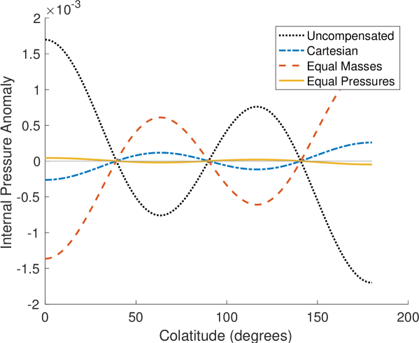
Figure 1: Comparison of internal pressure anomalies ($\delta p/\bar{p}$) for various basal topography solutions. Zero pressure anomaly means zero lateral pressure gradients along the equipotential surface $E_{d}\left(\theta,\phi\right)$. The dotted black line illustrates the pressure anomaly resulting from imposing the surface topography $H_{t30}$ without imposing any compensating isostatic root (i.e., with $H_{b30}=0$). The colored lines illustrate the pressure anomalies obtained when the isostatic root topography ($H_{b30}$) is computed via equations (1) (Cartesian isostatic balance; dash-dotted blue), (2) (equal mass in equal columns; dashed red), and (3) (equal pressures at depth; solid gold).

When compensation depths are shallow, $g_{t}\approx g_{b}$ and $R_{t}\approx R_{b}$, so that equations (2) and (3) both reduce to the usual Cartesian form of the isostatic balance. However, when compensation depths become non-negligible fractions of the body’s total radius, equations (1), (2), and (3) begin to diverge. When the crustal density is less than $\sim 70\%$ of the body’s bulk density, then $g_{t}<g_{b}$ (section S1.5, Figure S1), meaning that equation (1) generally overestimates the amplitude of the basal topography. When the crustal density is more than $\sim 70\%$ of the body’s bulk density (as is likely the case for Mars, for example), $g_{t}$ may be larger than $g_{b}$, and so equation (1) could underestimate the amplitude of the basal topography. However, of the three equations, (2) always yields the largest (most overestimated) isostatic roots because $R_{t}>R_{b}$ and because, assuming density does not increase with radius, $\bar{\rho}\leq\bar{\rho}_{b}$ (section S1.5).

3 Implications

3.1 Spectral Admittance

In combined studies of gravity and topography, it is common to use the spectral admittance as a means of characterizing the degree or depth of compensation [e.g., Wieczorek, 2015]. The mass associated with any surface topography (represented using spherical harmonic expansion coefficients, $H_{tlm}$) produces a corresponding gravity anomaly. However, if the topography is compensated isostatically—that is, if there is some compensating basal topography ($H_{blm}$)—the gravity anomaly can be reduced.

Using equation (S13), we can compute the surface gravity anomaly caused by the topography at the top and bottom of the crust, yielding

$$g_{lm}=\frac{l+1}{2l+1}4\pi G\left(\rho_{c}H_{tlm}+\Delta\rho H_{blm}\left(\frac{R_{b}}{R_{t}}\right)^{l+2}\right)$$ (11)

where again, $\rho_{c}$ is the density of the crust, $\Delta\rho$ is the density contrast at the crust/mantle interface, and where we have neglected any contributions that may arise from asymmetries on deeper density interfaces.

Taking the degree-$l$ admittance, $Z_{l}$, to be the ratio of gravitational acceleration ($g_{lm}$) to topography ($H_{tlm}$), and assuming complete Airy compensation, with the basal topography ($H_{blm}$) computed via the “equal masses” model, equation (2), we have

$$Z_{l}=\frac{l+1}{2l+1}4\pi G\rho_{c}\left(1-\left(\frac{R_{b}}{R_{t}}\right)^{l}\right)$$ (12)

Equation (12) is commonly used to generate a model admittance spectrum under the assumption of complete Airy compensation. Comparison of the model admittance with the observed admittance, along with an assumption about the crustal density then allows for an estimate of the compensation depth, $d=R_{t}-R_{b}$.

However, when we instead compute the basal topography using the “equal pressures” equation (3), we obtain

$$Z_{l}=\frac{l+1}{2l+1}4\pi G\rho_{c}\left(1-\left(\frac{g_{t}}{g_{b}}\right)\left(\frac{R_{b}}{R_{t}}\right)^{l+2}\right)$$ (13)

where again $g_{t}/g_{b}$ is given by equation (10).

Compared with equation (13), equation (12) will always lead to an overestimate of the compensation depth. That is, at any given spherical harmonic degree, using equation (13) yields the same admittance with a smaller compensation depth (Figure 2a). Equivalently, for any given compensation depth, the model admittance spectrum computed via equation (13) is larger than that obtained via equation (12) (Figure 2b). The discrepancy is always greatest at low spherical harmonic degrees (e.g., focusing on degree 3, and assuming that $\rho_{c}/\bar{\rho}=0.6$, would yield a compensation depth estimate that is roughly $\sim 50\%$ too large) and vanishes in the short wavelength limit (e.g., the compensation depth overestimate reduces to $<5$% for $l>50$).

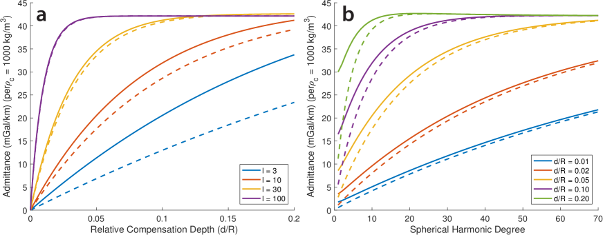
Figure 2: Admittance assuming Airy compensation. (a) Admittance as a function of relative compensation depth ($d/R$) for various example spherical harmonic degrees. (b) Spectral admittance for various examples of relative compensation depths. Dashed lines show admittance as computed via (12), which assumes equal masses in equal columns. Solid lines show admittance as computed via (13), which eliminates lateral pressure gradients at depth. The “equal masses” conception of isostasy always leads to underestimating the admittance, especially at low spherical harmonic degrees (long wavelengths). In both panels, admittance is normalized to an assumed crustal density of $1000\,\mathrm{kg/m^{3}}$ (i.e., if the crustal density is $2000\,\mathrm{kg/m^{3}}$, all admittance values double). Equation (13) also depends weakly on the internal density structure, which is here arbitrarily defined by $\rho_{c}/\bar{\rho}=0.6$.

For clarity and simplicity, we have not included the finite amplitude (or terrain) correction [e.g., Wieczorek and Phillips 1998] in the above admittance equations. When the topographic relief is a non-negligible fraction of the body’s radius, it may be important to include this effect, which will in general lead to larger admittances. However, the point of this paper is not so much to advocate the use of equation (13) in the admittance calculation, but rather, more fundamentally, to advocate the use of equation (3) in computing the basal topography.

It is worth emphasizing that the degree-2 admittance is complicated by the effects of rotational and possibly tidal deformation. A meaningful admittance calculation for degree-2 requires first removing the tidal/rotational effects from both the gravity and topography signals. Only the remaining, non-hydrostatic, signals should then be used in the admittance calculation. Unfortunately, determination of the hydrostatic components of the degree-2 gravity and topography signals requires knowledge of the body’s interior structure, which may not be readily available. In such cases, the easiest option would be to simply exclude the degree-2 terms in the admittance analysis. Alternatively, one might appeal to self-consistency arguments to constrain the internal structure and admittance simultaneously [e.g., Iess et al. 2014].

3.2 Geoid-to-Topography Ratio (GTR)

A closely related concept is the geoid-to-topography ratio (GTR), which has been used to estimate regional crustal thicknesses in situations where local isostasy can be reasonably expected [e.g., Wieczorek and Phillips 1997; Wieczorek and Zuber 2004]. Wieczorek and Phillips (1997) showed that the GTR is primarily a function of crustal thickness and can be computed from a compensation model according to

$$\text{GTR}=R_{t}\sum_{l=l_{\text{min}}}^{l_{\text{max}}}W_{l}Q_{l}$$ (14)

where $W_{l}$ is a weighting coefficient for degree-$l$, and $Q_{l}$ is a transfer function relating the degree-$l$ gravitational potential and topography coefficients

$$Q_{l}=\frac{C_{lm}}{H_{lm}}$$ (15)

The weighting coefficients reflect the fact that the geoid is most strongly affected by the longest wavelengths (lowest spherical harmonic degrees) and are constructed based on the topographic power spectrum, $S_{hh}\left(l\right)=\sum_{m=-l}^{l}H_{lm}^{2}$, according to

$$W_{l}=S_{hh}\left(l\right)/\sum_{i=l_{\text{min}}}^{l_{\text{max}}}S_{hh}\left(i\right)$$ (16)

(Wieczorek, 2015). $Q_{l}$ may be regarded as another expression for the spectral admittance ($Z_{l}$), except that it employs dimensionless gravitational potential coefficients rather than acceleration, and so we denote it here with a distinct symbol (also in accord with Wieczorek (2015)).

Neglecting the effects of topography on boundaries other than the surface and the crust/mantle interface, we can use equation (S12) to rewrite (15) as

$$Q_{l}=\frac{3}{2l+1}\left(\frac{\rho_{c}}{R_{t}\bar{\rho}}\right)\left(1+\frac{\Delta\rho H_{blm}}{\rho_{c}H_{tlm}}\left(\frac{R_{b}}{R_{t}}\right)^{l+2}\right)$$ (17)

Assuming complete Airy compensation, with the basal topography ($H_{blm}$) computed via the “equal masses” equation (2), we then have

$$\text{GTR}=\sum_{l=l_{\text{min}}}^{l_{\text{max}}}W_{l}\left(\frac{3}{2l+1}\right)\left(\frac{\rho_{c}}{\bar{\rho}}\right)\left(1-\left(\frac{R_{b}}{R_{t}}\right)^{l}\right)$$ (18)

If we instead compute the basal topography using the “equal pressures” equation (3), we obtain

$$\text{GTR}=\sum_{l=l_{\text{min}}}^{l_{\text{max}}}W_{l}\left(\frac{3}{2l+1}\right)\left(\frac{\rho_{c}}{\bar{\rho}}\right)\left(1-\left(\frac{g_{t}}{g_{b}}\right)\left(\frac{R_{b}}{R_{t}}\right)^{l+2}\right)$$ (19)

For reference, the linear dipole moment approximation (Ockendon and Turcotte, 1977; Haxby and Turcotte, 1978) can be written

$$\text{GTR}=\left(\frac{3}{2}\right)\left(\frac{\rho_{c}}{\bar{\rho}}\right)\left(1-\frac{R_{b}}{R_{t}}\right)$$ (20)

Each model thus suggests a different relationship between the GTR and the compensation depth (Figure 3). For shallow compensation depths (i.e., less than $\sim 4\%$ of the body’s radius assuming $\rho_{c}/\bar{\rho}=0.6$), the “equal pressures” conception of isostasy and the linear dipole moment approximation give similar results. For deeper compensation depths, the dipole moment approach begins to overestimate the GTR. In all cases, the “equal masses” approach underestimates the GTR, and therefore leads to an overestimate of the compensation depth (Figure 3).

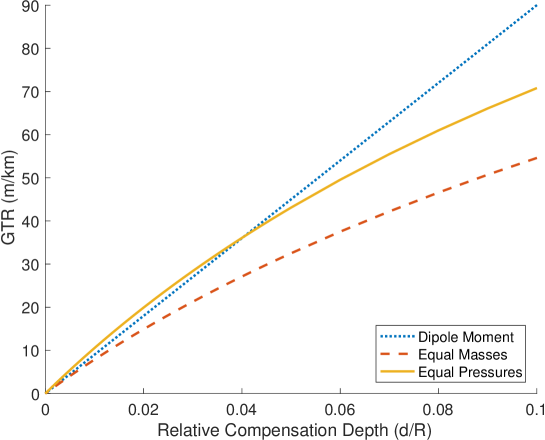
Figure 3: Geoid-to-Topography Ratio (GTR) as a function of relative compensation depth ($d/R$). Dotted blue line shows GTR computed via (20), using the linear dipole moment approximation. Dashed red line shows GTR computed via (18), which assumes equal masses in equal columns. Solid gold line shows GTR computed via (19), which avoids lateral pressure gradients at depth. The internal density structure is again arbitrarily defined by $\rho_{c}/\bar{\rho}=0.6$. The sum in (14) is taken from $l_{\text{min}}=3$ to $l_{\text{max}}=70$. The weighting coefficients are obtained from (16) by assuming a synthetic power spectrum defined by $S_{hh}=Al^{-1.5}$, where $A$ is an arbitrary constant. (cf. Figure 3a in Wieczorek and Phillips (1997) and Figure 1 in Wieczorek and Zuber (2004).)

3.3 Application to the Moon, Mars, and Icy Satellites

Here we consider a few realistic examples to illustrate how crustal thickness estimates differ when one adopts the “equal pressures” rather than the “equal masses” model. Note that the “equal pressures”-based crustal thickness values discussed in this section should not be taken as definitive new estimates. There are many subtleties to the interpretation of gravity and topography data that we have ignored here. The tools discussed in sections 3.1 and 3.2 will comprise only one component of any meaningful analysis of planetary crusts. Wieczorek and Zuber (2004), for instance, provide a comprehensive analysis that incorporates geochemical and mechanical equilibrium considerations to complement their GTR analysis. An updated estimate of the Martian highlands crustal thickness would require careful consideration of a wide range of relevant factors and an exploration of the permissible parameter space. Here, we wish only to illustrate, using a few specific examples, the importance of adjusting the admittance and GTR components of the analysis to incorporate the “equal pressures” isostatic equilibrium model rather than the “equal masses” model.

For the case of the nearside lunar highlands, Wieczorek and Phillips (1997) obtained geoid-to-topography ratios (GTRs) of roughly $14-34\,\mathrm{m/km}$. Taking the case of a single layer crust (Wieczorek and Phillips (1997) also considered dual-layer crusts), with a density of $2900\,\mathrm{kg/m^{3}}$ ($\rho_{c}/\bar{\rho}\approx 0.87$), this yields a crustal thickness estimate of roughly $22-61\,\mathrm{km}$ when the topography is assumed to be in isostatic equilibrium in the “equal masses” sense. Adopting the “equal pressures” model instead leads to crustal thickness estimates of $18-48\,\mathrm{km}$, suggesting that the “equal masses” model overestimates the crustal thickness by up to $\sim 27\%$ in this case (section S3.1, Figure S6a). For the Martian highlands, Wieczorek and Zuber (2004) obtained GTRs of roughly $13-19\,\mathrm{m/km}$, corresponding to crustal thicknesses of roughly $48-73\,\mathrm{km}$, assuming a crustal density of $2900\,\mathrm{kg/m^{3}}$ ($\rho_{c}/\bar{\rho}\approx 0.74$) and adopting the “equal masses” approach. The “equal pressures” model instead leads to crustal thicknesses of roughly $44-66\,\mathrm{km}$, not as dramatically different as in the case of the lunar highlands, but still indicating that the “equal masses” model overestimates the crustal thickness by $\sim 10\%$ in the case of the Martian highlands (section S3.1, Figure S6b).

For icy bodies, the ice shell’s density can be a considerably smaller fraction of the bulk density, leading to smaller $g_{t}/g_{b}$ ratios and therefore even more pronounced differences between the “equal masses” and “equal pressures” isostasy models (Figure S3). In the case of Europa, for example, a crustal density of $930\,\mathrm{kg/m^{3}}$ corresponds to $\rho_{c}/\bar{\rho}\approx 0.31$, leading the crustal thickness estimates to differ by a factor of roughly two at the lowest spherical harmonic degrees. For Encleadus ($\rho_{c}/\bar{\rho}\approx 0.58$, assuming $\rho_{c}=930\,\mathrm{kg/m^{3}}$), where the degree-2 and -3 gravity terms have been measured based on a series of Cassini flybys, Iess et al. (2014) were able to obtain a degree-3 admittance of $14.0\pm 2.8\,\mathrm{mGal/km}$, which allows for a crustal thickness estimate of $30\pm 6\,\mathrm{km}$, adopting the “equal masses” model. Adopting the “equal pressures” model instead leads to a remarkably different estimate of just $17\pm 4\,\mathrm{km}$ (section S3.2, Figure S7).

4 Conclusions

To the extent that isostatic equilibrium is a useful model for the state of mature planetary crusts, where broad topographic loads are supported mainly by buoyancy, it should be taken to mean a state in which hydrostatic (or lithostatic) pressures are equal along equipotential surfaces within the relatively low viscosity mantle. However, it is common in the literature to define isostatic equilibrium as the requirement that columns of equal width contain equal masses. Whereas these two definitions would be equivalent in a Cartesian framework, we have shown here that they are not equivalent in a spherical geometry (section 2). We have demonstrated that adopting the “equal masses” model leads to lateral pressure gradients that can be nearly as large (though opposite in sign) as if there were no isostatic compensation at all (Figure 1). We further showed that the “equal masses” model leads to an overestimate of either the compensating basal topography in the case of Airy compensation (section 2), or the compensating lateral crustal density variations in the case of Pratt compensation (section S2).

In combined studies of gravity and topography, using an “equal masses” model leads to an overestimate of the compensation depth (Figures 2 and S4). The discrepancy is always most significant at the lowest spherical harmonic degrees (longest wavelengths) and increases as the crustal density becomes a smaller fraction of the body’s bulk density. As examples, we showed that, in the case of the lunar and Martian highlands, the “equal masses” model could overestimate the crustal thicknesses by $\sim 27\%$ and $\sim 10\%$, respectively. For the case of Enceladus, where the compensation depth may be on the order of $10\%$ of the radius and where the ice shell density is roughly $58\%$ of the bulk density, the “equal masses” model may overestimate the shell thickness by nearly a factor of two. In the case of asymmetric loads (odd harmonics), we additionally note that the “equal masses” and “equal pressures” models will lead to distinct center of mass-center of figure offsets, a factor that could be important for smaller bodies.

Whereas, for the sake of clarity, we have focused here on the end-member case of complete isostatic equilibrium (purely buoyant support), the distinction between “equal masses” and “equal pressures” remains important for models in which the topography is supported by a combination of both buoyancy and elastic flexure—a topic that is beyond the scope of this work. While we acknowledge the limitations of the very concept of isostatic equilibrium (see Introduction), our goal here is merely to ensure that isostasy models at least correspond to what they are intended to mean—no lateral flow at depth when topographic loads are supported entirely by buoyancy. That is, in order to be consistent with the basic principle of isostasy, we must be sure to use the “equal pressures” model presented here and not the “equal masses” model. Beyond this simple picture, a fully self-consistent model of a planetary crust and its topography requires consideration of its loading history (i.e., where and when the loads were emplaced), the state of internal stresses (and failures) through time, and the potentially time-varying rheology of the relevant materials, within both the crust and the underlying mantle. Such models could be highly valuable, but only where sufficient clues are available to meaningfully constrain these many factors. In the absence of such information, the condition of isostatic equilibrium, as we have presented it here, is likely to remain a useful model, at least as a reference end member case.