Self-assembly of colloidal molecules due to self-generated flow

Abstract

The emergence of structure through aggregation is a fascinating topic and of both fundamental and practical interest. Here we demonstrate that self-generated solvent flow can be used to generate long-range attractions on the colloidal scale, with sub-pico Newton forces extending into the millimeter-range. We observe a rich dynamic behavior with the formation and fusion of small clusters resembling molecules, the dynamics of which is governed by an effective conservative energy that decays as $1/r$. Breaking the flow symmetry, these clusters can be made active.

Colloidal particles acting as “big” artificial atoms have been instrumental in studying microscopic processes in condensed matter, from the kinetics of crystallization Palberg (2014) to the vapor-liquid interface Aarts et al. (2004). Due to their size, colloidal particles are observable directly in real space. Moreover, interactions are widely tunable, ranging from hard spheres to long-range repulsive, short-range attractive, and dipolar Royall et al. (2003); Yethiraj (2007). Consequently, colloidal particles can be assembled into a multitude of different structures: from clusters Meng et al. (2010); Perry et al. (2015); Demirörs et al. (2015) and stable molecules Manoharan et al. (2003); Sacanna et al. (2010) composed of a few particles to extended bulk structures like ionic binary crystals Leunissen et al. (2005). In addition, self-assembly into useful superstructures can be controlled by factors such as confinement de Nijs et al. (2015) and particle shape Glotzer and Solomon (2007), which make colloids a versatile and fascinating form of matter Manoharan (2015).

What is still missing are truly long-range attractions of like-charged (or uncharged) identical colloidal particles. There is much interest in the basic statistical physics of systems with such interactions, which play a role in gravitational collapse, two-dimensional elasticity, chemotactic collapse, quantum fluids, and atomic clusters Campa et al. (2009). One proposed realization are colloidal particles trapped at an interface Ghezzi and Earnshaw (1997) that experience screened, long-range attractions due to capillary fluctuations of the interface Bleibel et al. (2011). The attractive interactions then correspond to Newtonian gravity in two dimensions. Complex patterns are also known to arise for bacteria due to long-range chemotactic interactions Budrene and Berg (1991). Critical long-range Casimir forces have been reported for colloidal particles in a binary solvent Hertlein et al. (2008), which are tunable by temperature and surface chemistry. Finally, a recent theoretical proposal are catalytically active colloidal particles that interact through producing or consuming chemicals Soto and Golestanian (2014, 2015). For simple diffusion the concentration profile of a chemical decays as inverse distance, implying long-range interactions that can be tuned through activity (how chemicals are produced or consumed) and mobility (how particles react to gradients).

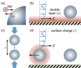
Figure 1: Long-range interactions through flow. (a) The colloidal particles release hydrogen ions (H⁺), which are exchanged with residual cationic impurities (here Na⁺). Different ion mobilities generate local electric fields $E$ that slow the hydrogen ions and accelerate the impurities to maintain overal electro-neutrality. (b) In the double layer of the substrate these fields generate electro-osmotic flow with solvent velocity $v_{\text{s}}$ towards the particle. (c) For two particles a distance $r$ apart, the higher H⁺ concentration in the space between particles reduces the gradient and leads to an asymmetric flow. (d) In the double layer of the particles, the same effect leads to electro-phoretic flow.

Here, we implement long-range attractions through hydrodynamic flows coupling suspended particles Banerjee et al. (2016); Feldmann et al. (2016). We report on experiments using spherical ion exchange resin particles sedimented to the negatively charged substrate. The particles have diameters of $15\,\mathrm{\mu m}$, for which Brownian diffusion is practically negligible on the experimental time scale. They interact due to self-generated local flow, resulting in an effective long-range $1/r$ attraction as expected for three-dimensional unscreened gravity. Our present understanding of the mechanism responsible for their aggregation can be summarized as follows Anderson (1989); Niu et al. (2016): By exchanging residual cationic impurities for stored hydrogen ions (Fig. 1a), the particles generate a concentration profile $c$ that decays away from the particles. Different diffusion coefficients of the exchanged cations and the released ions locally generate diffusio-electric fields which retain overall electro-neutrality by slowing the outward drift of hydrogen ions and accelerating the inward drift of impurities.

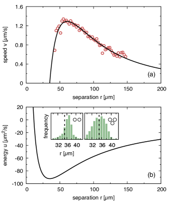
Figure 2: Effective pair potential. (a) Drift velocity $v(r)$ of two particles with separation $r$ (symbols). The line is the free fit to $v(r)=2u^{\prime}(r)$ with $u^{\prime}(r)$ denoting the derivative of Eq. (2). (b) The resulting effective pair potential $u(r)$. Insets: Histograms of the fluctuating bond length of dimers (left) and trimers (right), where the dashed line indicates the minimum $r_{0}\simeq 35\,\mathrm{\mu m}$ of the fitted effective potential.

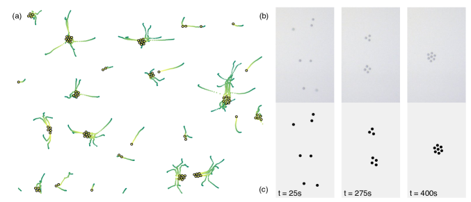
Figure 3: Dynamics of assembly. (a) Experimental particle traces and the configuration reached after $5\,\mathrm{min}$ (discs). (b,c) Consecutive snapshots from experiment (b) and a single simulation run (c) showing the formation of two clusters in their ground state (middle) and a large cluster with $n=7$ particles (right). The simulations have been initialized with the positions extracted from the first experimental snapshot.

The total system composed of solvent, ions, and colloidal particles is clearly out of thermal equilibrium through the free energy released by solvating the hydrogen ions, which drives the flow. However, appealing to a scale separation between particles and solvent, our crucial assumption will be that the motion of the particles themselves can be described by

$$\dot{\mathbf{r}}_{i}=-\nabla_{i}U+\boldsymbol{\eta}_{i},$$ (1)

where $U=\sum_{i<j}u(\mathbf{r}_{i}-\mathbf{r}_{j})$ is a conservative potential, $u(r)$ is the pair potential Eq. (2), and $\boldsymbol{\eta}_{i}$ models the noise with zero mean and correlations $\langle\boldsymbol{\eta}_{i}(t)\boldsymbol{\eta}_{j}^{T}(t^{\prime})\rangle=2D_{\text{eff}}\mathbf{1}\delta_{ij}\delta(t-t^{\prime})$.

The relative velocity of two particles with separation $\mathbf{r}=\mathbf{r}_{1}-\mathbf{r}_{2}$ is $v(r)=\langle(\mathbf{r}/r)\cdot(\dot{\mathbf{r}}_{1}-\dot{\mathbf{r}}_{2})\delta(|\mathbf{r}|-r)\rangle=2u^{\prime}(r)$ after inserting Eq. (1). Hence, we have direct access to the interactions $u(r)$ through measuring a dynamic quantity, the approach velocity $v(r)$ as shown in Fig. 2a. Approaching each other, the speed increases as expected but reaches a maximum at about $r\simeq 60\,\mathrm{\mu m}$ before it drops rapidly.

This behavior can be rationalized by considering the generated flows in more detail. In the double layer of the substrate, the local fields generate electro-osmotic flow of the solvent since the negative substrate is screened by an excess of positive charges (Fig. 1b). The motion of the particles is determined by the slip velocity $v_{\text{s}}=-\mu_{\text{p}}\nabla c$ with ion concentration field $c$ and phoretic mobility $\mu_{\text{p}}$ Anderson (1989), whereby our measured particle velocities are consistent with a constant mobility. For an isolated particle, the solvent flow is approaching symmetrically and no net motion results (the particle can be regarded as a sink in two dimensions; of course, the solvent is incompressible with backflow out of the plane of the substrate). For two particles, the hydrogen ion concentration is increased in the space between the particles, which reduces the gradient (with respect to the particles’ surfaces) and thus the flow velocity. Hence, the flow on each particle now becomes asymmetric, resulting in an apparent attraction (Fig. 1c). Basically the same mechanism acts in the double layer of the particles but now leads to electro-phoretic motion. The particles themselves are (slightly) negatively charged due to the release of cations. The field generated by the concentration gradient of the other particle again generates a solvent flow, however, now particle and solvent taken together are force-free, which leads to a particle speed in the opposite direction of the field (Fig. 1d).

For purely diffusive ion motion one would expect the concentration to decay as $c(r)\sim 1/r$, but measurements of the pH reveal a more complicated behavior (these measurements had to be performed for a larger particle, see Supplemental Material sm , but we expect the qualitative features to be the same for the smaller particles used here). While there is indeed a $1/r$ decay regime, closer to the ion exchange particle it changes to a slower decay that is well described as exponential. We speculate that this accumulation is caused by the local fields slowing down outward moving ions. We model this effect through a term resembling screening although we stress that it originates from the flow and not electrostatics. Combining both flows, the functional form of the potential reads

$$u(r)=-\frac{\gamma}{r}+\frac{\alpha}{r}e^{-r/\xi}$$ (2)

with three free parameters: the prefactors $\gamma$ and $\alpha$, and the screening length $\xi$. As shown in Fig. 2a, this function describes the experimental data very well. From the fit we obtain $\gamma\simeq 6120\,\mathrm{\mu m^{3}/s}$, $\alpha\simeq 8805\,\mathrm{\mu m^{3}/s}$, and $\xi\simeq 31.4\,\mathrm{\mu m}$. The pair potential $u(r)$ plotted in Fig. 2b has a minimum at $r_{0}\simeq 35\,\mathrm{\mu m}$. As shown in the inset of Fig. 2b, $r_{0}$ agrees well with the maximum of the distributions of bond length $r$ for dimers and trimers.

Usually, overdamped motion is described by a product of particle mobility and the gradient of the potential energy. Since we do not have access to these terms separately, we treat $u(r)$ as an effective “energy” absorbing the phoretic mobility $\mu$, with $u(r)$ thus having units of a diffusion coefficient. Nevertheless, we can estimate physical energies employing the bare particle mobility $\mu_{0}$, which quantifies the forces needed to move a single particle through the solvent with desired speed. For our particles in water its value is $\mu_{0}\simeq 7.8\,\mathrm{\mu m/(s\cdot pN)}$, yielding forces between particles of order $0.1\,\mathrm{pN}$. With $u(r_{0})\simeq-92.34\,\mathrm{\mu m^{2}/s}$, the corresponding bond dissociation energy would thus be $E_{\text{b}}=|u(r_{0})|/\mu_{0}\simeq 7000\,\mathrm{kJ/mol}$.

The final ingredient for our theoretical model is an effective temperature, which we extract from the measured bond fluctuations. First, from the distribution of the bond length $r$ for dimers we determine its variance $\text{Var}(r)\simeq 3.57\,\mathrm{\mu m^{2}}$. Assuming that these vibrations are effectively equilibrated allows us to determine the analog of a temperature, $D_{\text{eff}}\approx\text{Var}(r)u^{\prime\prime}(r_{0})\simeq 0.3\,\mathrm{\mu m^{2}/s}$. We test this assumption for three particles, for which a quick calculation predicts that the harmonic bond fluctuations are $\frac{5}{3}$ times larger sm . The predicted value $5.95\,\mathrm{\mu m^{2}}$ is only slightly smaller than the measured variance $6.25\,\mathrm{\mu m^{2}}$, the difference of which is due to anharmonic higher-order vibrations.

Our suspension of ion exchange particles is not stationary but slowly collapses to a close-packed state due to the long-range interactions. Starting from a homogeneous density profile, during this process we observe the formation of colloidal clusters (“molecules”) with $n$ particles. This assembly happens autonomously in contrast to prefabricated colloidal molecules Ebbens et al. (2010); Ni et al. (2017). While metastable, single clusters can be observed up to minutes, which allows in principle to study in detail different isomers and the “reactions” by which larger clusters form (more details are given as Supplemental Material sm ). In Fig. 3a we show the first few minutes of this process for a dilute suspension. The experiments were carried out with $60-90$ particles within a field of view corresponding to an area fraction of approx. $0.25\%$. Without adjustable parameters, the observed dynamics are reproduced through the model described by Eq. (1). In Fig. 3b we show a sequence of experimental snapshots for seven particles. We then perform simulations of the model using the extracted particle positions from the first experimental frame as initial positions. As shown in Fig. 3c, the simulations agree with the experiments on the same time scale. While for repeated simulation runs the positions differ due to the noise, the average behavior is consistent.

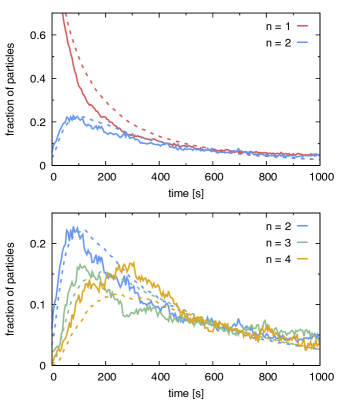
Figure 4: Time evolution of cluster populations $N_{n}(t)/N$. Solid lines correspond to experimental data (averaged over several experiments), dashed lines to the simulation results of the theoretical model with $N=80$ particles.

This fit-free quantitative agreement is corroborated by the time evolution of the fraction of clusters with weight $n$. From the analysis of the experiments, we extract the fraction $N_{n}(t)/N$ of particles residing in clusters with $n$ particles. The range of $N$ is between 60 and 90, and to improve statistics we average over all experiments. We repeat the same analysis with the theoretical model for $N=80$, the comparison of which is shown in Figure 4. The qualitative behavior is that of irreversible aggregation as described through the Smoluchowski coagulation equation Aldous (1999), with a steady decrease of the monomer concentration and peaks for the $n$-mers that become flatter and shifted to later times for increasing weight $n$.

As demonstrated, for a one-component suspension of ion exchange particles in moderate flow the dynamics of the particles alone is effectively described through a conservative potential. However, for larger aggregates also the flow increases, leading to deviations from the predicted behavior (e.g. particles are lifted and pushed into the second layer). With even larger flows, particles are observed to spontaneously break the flow symmetry and become self-propelled. Another strategy is to explicitly break symmetry through mixtures of particles with different sizes or shapes, or mixtures of activated and passive particles Reinmüller et al. (2013). Here we explore the consequences of adding anionic ion exchange particles of similar size but releasing OH^- ions, for which we again observe the assembly of low-weight clusters. This is shown exemplary in Fig. 5 for two cationic particles and one anionic particle, which assemble into a trimer. As predicted in Ref. 19, the geometry together with the different mobilities/activities leads to a self-propelled complex. This can be seen through determining the center-of-mass speed of the three particles, which clearly shows a transition to a constant speed once the trimer has assembled.

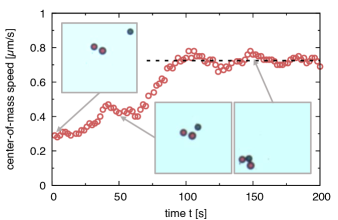
Figure 5: Transition to self-propelled motion. Plotted is the center-of-mass speed of three particles, two cationic and one anionic, which accelerate once assembled into a trimer (at $t\approx 50\,\mathrm{s}$). For times $t=0\,\mathrm{s}$, $50\,\mathrm{s}$, and $150\,\mathrm{s}$ snapshots are shown with cationic particles in red and anionic particles in blue. The field of view is the same for all snapshots. The dashed line indicates the final speed of the trimer.

To conclude, we have shown that ion exchange particles close to a charged substrate generate flows that lead to effectively conservative, long-range interactions. Autonomous flow-driven assembly through long-range attractions might enable novel non-equilibrium materials and strategies in self-assembly, in particular on intermediate scales for which thermal motion has become negligible but which cannot be manipulated directly. Moreover, through changing composition one may generate asymmetric flow. The resulting directed motion of colloidal particles in combination with volume exclusion leads to fascinating dynamic behavior ranging from clustering Buttinoni et al. (2013) and the formation of “living crystals” Palacci et al. (2013) to schooling and swarming Yan et al. (2016). Our results demonstrate how one can implement strategies to control and engineer interactions and directed motion on the same footing Zhang et al. (2016), which is a step towards designing active particles that can perform dynamical tasks such as transport of cargo Sundararajan et al. (2008); Baraban et al. (2012). Concerning the size of the particles used here, we note that there is no conceptual barrier to using smaller particles, the main issue being the ion exchange rate and ion capacity of singe particles that determines the flow strength and the time over which the flow is being generated.

Supplementary Information

I Experiments

The particles are cationic ion exchange resin particles (CK10S, Mitsubishi Chemical Corporation, Japan) with diameter $2a=15.3\pm 3.0\,\mathrm{\mu m}$ and counter ions Na⁺. Prior to experiments, the particles were washed with $20\,wt\%$ hydrochloride acid solution to exchange the counter ions into H⁺. Then we rinsed with doubly deionized water several times until solution pH of $\sim 7$ and dried at $80^{\circ}\,\mathrm{C}$ for 2 h. The sample cell was built from a circular Perspex ring (inner diameter of $20\,\mathrm{mm}$, height of $1\,\mathrm{mm}$) fixed to microscopy slides by hydrolytically inert epoxy glue and dried for 24 h before use. The glass slides were washed with alkaline solution (Hellmanex®III, Hellma Analytics) for 30 min under sonication, and subsequently rinsed with tap water and deionized water for several times.

In a typical experiment, a weighted amount of particles was dispersed into doubly deionized water. Subsequently, 400 $\mu$-liters of particle suspension was added into the sample cell. The cell was covered immediately to avoid contamination. Particles settled to the bottom of the cell within minutes. Movies were then taken at a frame rate of 0.5 Hz using an inverted scientific microscope (DMIRBE by Leica, Germany). Particles were tracked through extracting the perimeter using a home-written Python script. The velocity $v(r)$ of two approaching particles was averaged over 160 pairs with any other particle at least 10 times their diameter away.

In a second set of experiments we have added anionic ion exchange resin particles (CA08S, Mitsubishi Chemical Corporation, Japan) with diameter $2a=15.1\pm 0.3\,\mathrm{\mu m}$ and counter ions Cl^-. Before use, particles were washed with concentrated sodium hydroxide (NaOH) to exchange the counter ions into OH^- and subsequently washed with deionized water until the pH of the solution reached about 7. To distinguish cationic ion exchange resin and anionic ion exchange resin, tiny amount of pH indicator solution (pH 4-10, Sigma-Aldrich) was added to mark them redish and bluish, respectively.

II Hydrogen ion concentration

We determine the pH profile around an ion exchange particle with diameter $45\,\mathrm{\mu m}$ using a mixture of Universal indicator solutions (1:3 volume ratio of pH 0-5 and pH 4-10, Sigma-Aldrich, Inc). As the concentration of proton decreases, the color ratio of blue-to-red decreases monotonically. Thus, measuring the blue-to-red color ratio at fixed pH, we get a calibration curve. Applying this calibration curve to every pixel around ion exchange particle, we determine the proton concentration. The color images were recorded using a consumer DSLR (D700, Nikon, Japen) mounted on an inverted scientific microscope (DMIRBE, Leica, Germany). Image recording starts $\sim 2\,\mathrm{s}$ after the ion exchange particle gets into contact with the indicator solution. The measured concentration $c(r,t)$ as a function of distance $r$ from the particle center and time $t$ after preparation is shown in Figure 6.

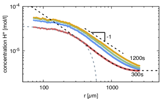
Figure 6: Concentration profiles $c(r,t)=10^{-\text{pH}}$ of hydrogen ions as a function of distance $r$ from the ion exchange particle for different times $t=300,660,900,1200\,\mathrm{s}$ (from bottom to top) after contact with water. Indicated are a fit to Eq. (3) (black dashed line), the initial exponential decay (gray dashed line), and the $1/r$ decay (straight dashed line) before the background concentration is approached.

A prediction for the concentration profile is given by the solution of the diffusion equation

$$\partial_{t}c(\mathbf{r},t)=D_{+}\nabla^{2}c(\mathbf{r},t)+\gamma\delta(\mathbf{r})$$

with ion diffusion coefficient $D_{+}$ and assuming a constant rate $\gamma$ with which ions are released. The solution is

$$c(r,t)=\frac{\gamma}{4\pi D_{+}r}\operatorname{erfc}\left(\frac{r}{2\sqrt{D_{+}t}}\right)+c_{\infty}$$ (3)

with background concentration $c_{\infty}$. From the fit of this expression to the decay of the concentration profile we obtain a background $\text{pH}\simeq 5.45$ and a diffusion coefficient $D_{+}\simeq 1300\,\mathrm{\mu m^{2}/s}$, which is reasonable for hydrogen ions given the fact that they are hydrated. Strikingly, the qualitative behavior changes when approaching the particle and the concentration profile decays much slower than what is expected from the simple diffusion picture. In fact, it can be fitted well by an exponential decay. This implies that outward moving ions are slowed, presumably through local electric fields generated in conjunction with other ions. The resulting solvent flow is thus more complex than $v_{\text{s}}\sim\nabla c\sim 1/r^{2}$, which is captured by the form of our effective pair potential, see the discussion in the main text.

III Bond vibrations in the trimer

While the suspension itself is non-stationary, for the bond vibrations we assume that an effective equilibrium has been reached described by the Boltzmann factor. We expand the energy

$$U\approx U_{0}+\frac{1}{2}\sum_{ij}^{2n}H_{ij}\delta x_{i}\delta x_{j}=U_{0}+\frac{1}{2}\sum_{\alpha=1}^{2n}\kappa_{\alpha}q_{\alpha}^{2},$$

where $\mathbf{H}$ is the $2n\times 2n$ Hessian matrix of second derivatives of the potential energy evaluated at the minimum energy configuration of the cluster with $n$ particles. It has $2n$ eigenvalues $\kappa_{\alpha}$, of which three are zero corresponding to translation and rotation in two dimensions. The other eigenvalues are the spring constants of the vibrational modes.

For $n=3$, the minimum energy configuration is an equilateral triangle and the Hessian becomes $\mathbf{H}=u^{\prime\prime}(r_{0})\mathbf{A}$ with constant matrix $\mathbf{A}$ (with non-zero eigenvalues $\frac{3}{2},\frac{3}{2},3$). The harmonic fluctuations of any edge can easily be calculated as

$$\langle|\mathbf{r}_{i}-\mathbf{r}_{j}-r_{0}\mathbf{\hat{\mathbf{r}}}_{ij}|^{2}\rangle=\sum_{\alpha}\langle q_{\alpha}^{2}\rangle=\sum_{\alpha}\frac{D_{\text{eff}}}{\kappa_{\alpha}}=\frac{5}{3}\frac{D_{\text{eff}}}{u^{\prime\prime}(r_{0})}$$

as used in the main text.

IV Metastable molecules

Figure 8 shows snapshots of structural arrangements sorted by their molecular weight from $n=3$ to $n=6$. We only show structures that persisted for at least $100\,\mathrm{s}$. We distinguish isomers assigning a structural fingerprint counting the number $n_{b}$ of particles with $b$ direct bonds. For every particle configuration (experiments and simulations) we first determine clusters of mutually bonded particles, where a particle pair $(i,j)$ forms a bond if the separation $|\mathbf{r}_{ij}|$ is smaller than the cutoff of $40\,\mathrm{\mu m}$. We then refine the bond network and only retain bonds between direct neighbors. A particle $j$ is a direct neighbor of $i$ if for all particles $k$ with distance $|\mathbf{r}_{ik}|<|\mathbf{r}_{ij}|$ the condition $\mathbf{r}_{ik}\cdot\mathbf{r}_{jk}>0$ holds (the enclosed angle is less than $\pi/2$ radians) Malins et al. (2013). For each cluster we count the number of particles $n_{b}$ with $b$ bonds, the vector of which forms a “fingerprint” based on which we identify the isomeric structure of the molecule.

The structures to the left in Figure 8 show the ground states minimizing the effective energy. From the eigenspectrum of vibrations we delineate (meta-)stable molecules (blue frames) from unstable molecules (red frames). For $n=3$ and $n=4$ the latter nevertheless occur with a non-vanishing probability since they are populated by reactions adding another monomer. We can identify these transition states easily by their “dangling bonds” with $n_{1}>0$. Transition states quickly rearrange into stable isomers for the same $n$. These are relatively long-lived – typically until another reaction occurs increasing the molecular weight – but we also observe spontaneous transitions between isomers (see Supplementary Movie 2 and Fig. 7). For $n=6$ we have four stable isomers. For short-range attractions counting only direct bonds, the structures II, III, and IV form the degenerate ground state manifold Perry et al. (2015). Due to the long-range attractions in our case, the degeneracy is lifted with the regular pentagon (I) representing the minimal energy configuration. While most transitions proceed through a slight shift of bonds, note that the transition $\text{IV}\to\text{III}$ involves breaking a bond with excited intermediate III^∗. Consequently, for the parallelogram (IV) we observe a higher population both in experiment and theory than one would expect from its energy alone.

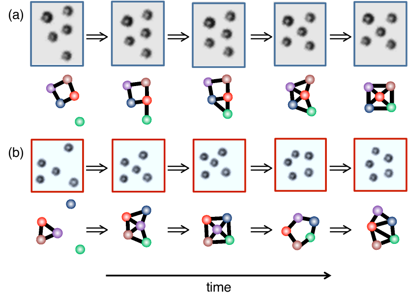
Figure 7: Two examples of structural changes for $n=5$ (see also Supplementary Movie 2). (a) Formation of a transition structure after addition of one monomer, which quickly relaxes to configuration 5-II. (b) Trimer plus two monomers again relaxing to 5-II but now followed by the reorganization into the ground state 5-I through pushing out the center particle.

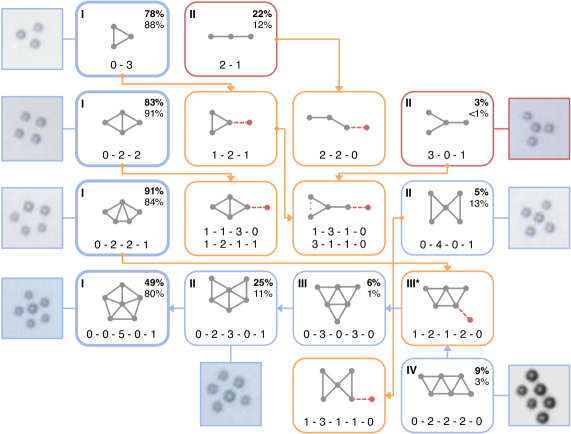
Figure 8: Colloidal “molecules”. Sketch of molecules with $n$ particles (from top $n=3$ to bottom $n=6$) and snapshots as observed in the experiments. Configurations with blue frames correspond to local energy minima (stable vibrations) whereas red frames indicate unstable configurations. The ground states are indicated to the left with thick frames. Also shown are examples for excited transition states (orange frames), which are characterized by at least one dangling bond (in red). Below every structure the structural fingerprint is given as the vector $n_{1}$–$n_{2}$–…counting the number of particles with one bond, two bonds, etc. For $n=6$, the blue arrows indicate favored transitions between the stable isomers. In the right corner we compare the population of that structure between experiment (top and bold) and simulation (bottom). Difference to 100% is the population of transition states.