Support vector machine and its bias correction in high-dimension, low-sample-size settings

Abstract

In this paper, we consider asymptotic properties of the support vector machine (SVM) in high-dimension, low-sample-size (HDLSS) settings. We show that the hard-margin linear SVM holds a consistency property in which misclassification rates tend to zero as the dimension goes to infinity under certain severe conditions. We show that the SVM is very biased in HDLSS settings and its performance is affected by the bias directly. In order to overcome such difficulties, we propose a bias-corrected SVM (BC-SVM). We show that the BC-SVM gives preferable performances in HDLSS settings. We also discuss the SVMs in multiclass HDLSS settings. Finally, we check the performance of the classifiers in actual data analyses.

1 Introduction

High-dimension, low-sample-size (HDLSS) data situations occur in many areas of modern science such as genetic microarrays, medical imaging, text recognition, finance, chemometrics, and so on. Suppose we have independent and $d$-variate two populations, $\pi_{i},\ i=1,2$, having an unknown mean vector $\mbox{\boldmath$\mu$}_{i}$ and unknown covariance matrix $\mbox{\boldmath$\Sigma$}_{i}\ (\geq\mbox{\boldmath{$O$}})$. We assume that $\mbox{\rm tr}(\mbox{\boldmath$\Sigma$}_{i})/d\in(0,\infty)$ as $d\to\infty$ for $i=1,2$. Here, for a function, $f(\cdot)$, “$f(d)\in(0,\infty)$ as $d\to\infty$” implies $\liminf_{d\to\infty}f(d)>0$ and $\limsup_{d\to\infty}f(d)<\infty$. Let $\Delta=\|\mbox{\boldmath$\mu$}_{1}-\mbox{\boldmath$\mu$}_{2}\|^{2}$, where $\|\cdot\|$ denotes the Euclidean norm. We assume that $\limsup_{d\to\infty}\Delta/d<\infty$. We have independent and identically distributed (i.i.d.) observations, $\mbox{\boldmath{$x$}}_{i1},...,\mbox{\boldmath{$x$}}_{in_{i}}$, from each $\pi_{i}$. We assume $n_{i}\geq 2,\ i=1,2$. Let $\mbox{\boldmath{$x$}}_{0}$ be an observation vector of an individual belonging to one of the two populations. We assume $\mbox{\boldmath{$x$}}_{0}$ and $\mbox{\boldmath{$x$}}_{ij}$s are independent. Let $N=n_{1}+n_{2}$.

In the HDLSS context, Hall et al. (2005), Marron et al. (2007) and Qiao et al. (2010) considered distance weighted classifiers. Hall et al. (2008), Chan and Hall (2009) and Aoshima and Yata (2014) considered distance-based classifiers. In particular, Aoshima and Yata (2014) gave the misclassification rate adjusted classifier for multiclass, high-dimensional data in which misclassification rates are no more than specified thresholds. On the other hand, Aoshima and Yata (2011, 2015a) considered geometric classifiers based on a geometric representation of HDLSS data. Ahn and Marron (2010) considered a classifier based on the maximal data piling direction. Aoshima and Yata (2015b) considered quadratic classifiers in general and discussed asymptotic properties and optimality of the classifies under high-dimension, non-sparse settings. In particular, Aoshima and Yata (2015b) showed that the misclassification rates tend to $0$ as $d$ increases, i.e.,

$$e(i)\to 0\ \ \mbox{as $d\to\infty$ for $i=1,2$}$$ (1)

under the non-sparsity such as $\Delta\to\infty$ as $d\to\infty$, where $e(i)$ denotes the error rate of misclassifying an individual from $\pi_{i}$ into the other class. We call (1) “the consistency property”. We note that a linear classifier can give such a preferable performance under the non-sparsity. Also, such non-sparse situations often appear in real high-dimensional data. See Aoshima and Yata (2015b) for the details. Hence, in this paper, we focus on linear classifiers.

In the field of machine learning, there are many studies about the classification in the context of supervised learning. A typical method is the support vector machine (SVM). The SVM has versatility and effectiveness both for low-dimensional and high-dimensional data. See Vapnik (2000), Schölkopf and Smola (2002), Hall et al. (2005), Hastie et al. (2009) and Qiao and Zhang (2015) for the details. Even though the SVM is quite popular, its asymptotic properties seem to have not been studied sufficiently. In this paper, we investigate asymptotic properties of the SVM for HDLSS data.

Now, let us use the following toy examples to see the performance of the hard-margin linear SVM given by (5). We set $N=20$ and $d=2^{s},\ s=5,...,11$. Independent pseudo random observations were generated from $\pi_{i}:N_{d}(\mbox{\boldmath$\mu$}_{i},\mbox{\boldmath$\Sigma$}_{i})$, $i=1,2$. We set $\mbox{\boldmath$\mu$}_{1}=\mbox{\boldmath{$0$}}$ and $\mbox{\boldmath$\mu$}_{2}=(1/3,...,1/3)^{T}$, so that $\Delta=d/9$. We considered three cases:

(a) $(n_{1},n_{2})=(10,10)$ and $\mbox{\boldmath$\Sigma$}_{1}=\mbox{\boldmath$\Sigma$}_{2}=\mbox{\boldmath{$I$}}_{d}$;

(b) $(n_{1},n_{2})=(6,14)$ and $\mbox{\boldmath$\Sigma$}_{1}=\mbox{\boldmath$\Sigma$}_{2}=\mbox{\boldmath{$I$}}_{d}$; and

(c) $(n_{1},n_{2})=(10,10)$, $\mbox{\boldmath$\Sigma$}_{1}=0.6\mbox{\boldmath{$I$}}_{d}$ and $\mbox{\boldmath$\Sigma$}_{2}=1.4\mbox{\boldmath{$I$}}_{d}$,

where $\mbox{\boldmath{$I$}}_{d}$ denotes the $d$-dimensional identity matrix. Note that $\Delta>|\mbox{\rm tr}(\mbox{\boldmath$\Sigma$}_{1})/n_{1}-\mbox{\rm tr}(\mbox{\boldmath$\Sigma$}_{2})/n_{2}|$ for (a) to (c). Then, from Theorem 1 in Hall et al. (2005), the classifier should hold (1) for (a) to (c). We repeated 2000 times to confirm if the classifier does (or does not) classify $\mbox{\boldmath{$x$}}_{0}\in\pi_{i}$ correctly and defined $P_{ir}=0\ (\mbox{or}\ 1)$ accordingly for each $\pi_{i}\ (i=1,2)$. We calculated the error rates, $\overline{e}(i)=\sum_{r=1}^{2000}P_{ir}/2000$, $i=1,2$. Also, we calculated the average error rate, $\overline{e}=\{\overline{e}(1)+\overline{e}(2)\}/2$. Their standard deviations are less than $0.0112$ from the fact that $\mbox{\rm Var}\{\overline{e}(i)\}=e(i)\{1-e(i)\}/2000\leq 1/8000$. In Figure 1, we plotted $\overline{e}(1)$, $\overline{e}(2)$ and $\overline{e}$ for (a) to (c). We observe that the SVM gives a good performance as $d$ increases for (a). Contrary to expectations, it leads undesirable performances both for (b) and (c). The error rates becomes small as $d$ increases, however, $\overline{e}(1)$ and $\overline{e}(2)$ are quite unbalanced. We discuss some theoretical reasons in Section 2.2.

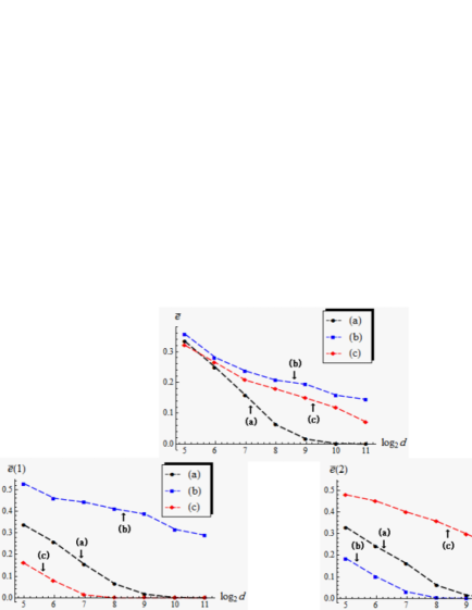
Figure 1: The performance of the SVM given by (5) in HDLSS settings. The left panel displays $\overline{e}(1)$, the right panel displays $\overline{e}(2)$ and the top panel displays $\overline{e}$. Their standard deviations are less than $0.0112$.

In this paper, we investigate the SVM in the HDLSS context. In Section 2, we show that the SVM holds (1) under certain severe conditions. We show that the SVM is very biased in HDLSS settings and its performance is affected by the bias directly. In order to overcome such difficulties, we propose a bias-corrected SVM (BC-SVM) in Section 3. We show that the BC-SVM improves the SVM even when $n_{i}$s or $\mbox{\boldmath$\Sigma$}_{i}$s are unbalanced as in (b) or (c) in Figure 1. In Section 4, we check the performance of the BC-SVM by numerical simulations and use the BC-SVM in actual data analyses. In Section 5, we discuss multiclass SVMs in HDLSS settings.

2 SVM in HDLSS Settings

In this section, we give asymptotic properties of the SVM in HDLSS settings. Since HDLSS data are linearly separable by a hyperplane, we consider the hard-margin linear SVM.

2.1 Hard-margin linear SVM

We consider the following linear classifier:

$$y(\mbox{\boldmath{$x$}})=\mbox{\boldmath{$w$}}^{T}\mbox{\boldmath{$x$}}+b,$$ (2)

where $w$ is a weight vector and $b$ is an intercept term. Let us write that $(\mbox{\boldmath{$x$}}_{1},...,\mbox{\boldmath{$x$}}_{N})=(\mbox{\boldmath{$x$}}_{11},...,\mbox{\boldmath{$x$}}_{1n_{1}},\mbox{\boldmath{$x$}}_{21},...,\mbox{\boldmath{$x$}}_{2n_{2}})$. Let $t_{j}=-1$ for $j=1,...,n_{1}$ and $t_{j}=1$ for $j=n_{1}+1,...,N$. The hard-margin SVM is defined by maximizing the smallest distance of all observations to the separating hyperplane. The optimization problem of the SVM can be written as follows:

$$\mathop{\rm argmin}\limits_{{\scriptsize\mbox{\boldmath{$w$}}},b}\frac{1}{2}\|\mbox{\boldmath{$w$}}\|^{2}\quad\mbox{subject to \ $t_{j}(\mbox{\boldmath{$w$}}^{T}\mbox{\boldmath{$x$}}_{j}+b)\geq 1$, $j=1,...,N$.}$$

A Lagrangian formulation is given by

$$L(\mbox{\boldmath{$w$}},b;\mbox{\boldmath$\alpha$})=\frac{1}{2}||\mbox{\boldmath{$w$}}||^{2}-\sum_{j=1}^{N}\alpha_{j}\{t_{j}(\mbox{\boldmath{$w$}}^{T}\mbox{\boldmath{$x$}}_{j}+b)-1\},$$

where $\mbox{\boldmath$\alpha$}=(\alpha_{1},...,\alpha_{N})^{T}$ and $\alpha_{j}$s are Lagrange multipliers. By differentiating the Lagrangian formulation with respect to $w$ and $b$, we obtain the following conditions:

$$\mbox{\boldmath{$w$}}=\sum_{j=1}^{N}\alpha_{j}t_{j}\mbox{\boldmath{$x$}}_{j}\ \mbox{ and }\ \sum_{j=1}^{N}\alpha_{j}t_{j}=0.$$

After substituting them into $L(\mbox{\boldmath{$w$}},b;\mbox{\boldmath$\alpha$})$, we obtain the dual form:

$$L(\mbox{\boldmath$\alpha$})=\sum_{j=1}^{N}\alpha_{j}-\frac{1}{2}\sum_{j=1}^{N}\sum_{k=1}^{N}\alpha_{j}\alpha_{k}t_{j}t_{k}\mbox{\boldmath{$x$}}_{j}^{T}\mbox{\boldmath{$x$}}_{k}.$$ (3)

The optimization problem can be transformed into the following:

$$\mathop{\rm argmax}\limits_{\mbox{\scriptsize$\mbox{\boldmath$\alpha$}$}}L(\mbox{\boldmath$\alpha$})$$

subject to

$$\alpha_{j}\geq 0,\ j=1,...,N,\ \mbox{ and }\ \sum_{j=1}^{N}\alpha_{j}t_{j}=0.$$ (4)

Let us write that

$$\hat{\mbox{\boldmath$\alpha$}}=(\hat{\alpha}_{1},...,\hat{\alpha}_{N})^{T}=\mathop{\rm argmax}\limits_{\mbox{\scriptsize$\mbox{\boldmath$\alpha$}$}}L(\mbox{\boldmath$\alpha$})\ \mbox{ subject to (\ref{2.3})}.$$

There exist some $\mbox{\boldmath{$x$}}_{j}$s satisfying that $t_{j}y(\mbox{\boldmath{$x$}}_{j})=1$ (i.e., $\hat{\alpha}_{j}\neq 0$). Such $\mbox{\boldmath{$x$}}_{j}$s are called the support vector. Let $\hat{S}=\{j|\hat{\alpha}_{j}\neq 0,\ j=1,...,N\}$ and $N_{\hat{S}}=\#\hat{S}$, where $\#A$ denotes the number of elements in a set $A$. The intercept term is given by

$$\hat{b}=\frac{1}{N_{\hat{S}}}\sum_{j\in\hat{S}}\Big{(}t_{j}-\sum_{k\in\hat{S}}\hat{\alpha}_{k}t_{k}\mbox{\boldmath{$x$}}_{j}^{T}\mbox{\boldmath{$x$}}_{k}\Big{)}.$$

Then, the linear classifier in (2) is defined by

$$\hat{y}(\mbox{\boldmath{$x$}})=\sum_{k\in\hat{S}}\hat{\alpha}_{k}t_{k}\mbox{\boldmath{$x$}}_{k}^{T}\mbox{\boldmath{$x$}}+\hat{b}.$$ (5)

Finally, in the SVM, one classifies $\mbox{\boldmath{$x$}}_{0}$ into $\pi_{1}$ if $\hat{y}(\mbox{\boldmath{$x$}}_{0})<0$ and into $\pi_{2}$ otherwise. See Vapnik (2000) for the details.

2.2 Asymptotic properties of the SVM in the HDLSS context

In this section, we consider the case when $d\to\infty$ while $N$ is fixed. We assume the following assumptions:

(A-i)

$\displaystyle\frac{\mbox{\rm Var}(\|\mbox{\boldmath{$x$}}_{ik}-\mbox{\boldmath$\mu$}_{i}\|^{2})}{\Delta^{2}}\to 0$ as $d\to\infty$ for $i=1,2$;

(A-ii)

$\displaystyle\frac{\mbox{\rm tr}(\mbox{\boldmath$\Sigma$}_{i}^{2})}{\Delta^{2}}\to 0$ as $d\to\infty$ for $i=1,2$.

Note that $\mbox{\rm Var}(\|\mbox{\boldmath{$x$}}_{ik}-\mbox{\boldmath$\mu$}_{i}\|^{2})=2\mbox{\rm tr}(\mbox{\boldmath$\Sigma$}_{i}^{2})$ when $\pi_{i}$ is Gaussian, so that (A-i) and (A-ii) are equivalent when $\pi_{i}$s are Gaussian.

Lemma 1.

Under (4), it holds that as $d\to\infty$

$$L(\mbox{\boldmath$\alpha$})=\sum_{j=1}^{N}\alpha_{j}-\frac{\Delta}{8}\Big{(}\sum_{j=1}^{N}\alpha_{j}\Big{)}^{2}\{1+o_{p}(1)\}-\frac{1}{2}\Big{(}\mbox{\rm tr}(\mbox{\boldmath$\Sigma$}_{1})\sum_{j=1}^{n_{1}}\alpha_{j}^{2}+\mbox{\rm tr}(\mbox{\boldmath$\Sigma$}_{2})\sum_{j=n_{1}+1}^{N}\alpha_{j}^{2}\Big{)}.$$

Let $\delta=\mbox{\rm tr}(\mbox{\boldmath$\Sigma$}_{1})/n_{1}+\mbox{\rm tr}(\mbox{\boldmath$\Sigma$}_{2})/n_{2}$ and $\Delta_{*}=\Delta+\delta$. Under the constraint that $\sum_{j=1}^{N}\alpha_{j}=C$ for a given positive constant $C$, we can claim that

$$\max_{\mbox{\scriptsize$\mbox{\boldmath$\alpha$}$}}\Big{\{}-\frac{1}{2}\Big{(}\mbox{\rm tr}(\mbox{\boldmath$\Sigma$}_{1})\sum_{j=1}^{n_{1}}\alpha_{j}^{2}+\mbox{\rm tr}(\mbox{\boldmath$\Sigma$}_{2})\sum_{j=n_{1}+1}^{N}\alpha_{j}^{2}\Big{)}\Big{\}}=-\frac{C^{2}}{8}\delta$$ (6)

when $\alpha_{1}=\cdots=\alpha_{n_{1}}=C/(2n_{1})$ and $\alpha_{n_{1}+1}=\cdots=\alpha_{N}=C/(2n_{2})$ under (4). Then, by noting that $\liminf_{d\to\infty}\{\mbox{\rm tr}(\mbox{\boldmath$\Sigma$}_{i})/(\Delta n_{i})\}>0$ for $i=1,2$, from Lemma 1 it holds that

$$\max_{\mbox{\scriptsize$\mbox{\boldmath$\alpha$}$}}L(\mbox{\boldmath$\alpha$})=-\frac{\Delta_{*}}{8}\Big{(}C-\frac{4+o_{p}(1)}{\Delta_{*}}\Big{)}^{2}\{1+o_{p}(1)\}+\frac{2+o_{p}(1)}{\Delta_{*}}$$ (7)

for given $C(>0)$. Hence, by choosing $C\approx 4/\Delta_{*}$, we have the maximum of $L(\mbox{\boldmath$\alpha$})$ asymptotically.

Lemma 2.

It holds that as $d\to\infty$

$$\hat{\alpha}_{j}=\frac{2}{\Delta_{*}n_{1}}\{1+o_{p}(1)\}\quad\mbox{for $j=1,...,n_{1}$};\quad\mbox{and}$$

$$\hat{\alpha}_{j}=\frac{2}{\Delta_{*}n_{2}}\{1+o_{p}(1)\}\quad\mbox{for $j=n_{1}+1,...,N$}.$$

Furthermore, it holds that as $d\to\infty$

$$\hat{y}(\mbox{\boldmath{$x$}}_{0})=\frac{(-1)^{i}\Delta}{\Delta_{*}}+\frac{\mbox{\rm tr}(\mbox{\boldmath$\Sigma$}_{1})/n_{1}-\mbox{\rm tr}(\mbox{\boldmath$\Sigma$}_{2})/n_{2}}{\Delta_{*}}+o_{p}\Big{(}\frac{\Delta}{\Delta_{*}}\Big{)}$$

when $$\mbox{\boldmath{$x$}}_{0}\in\pi_{i} i=1,2$$, .

Remark 1.

From Lemma 2, all the data points are the support vectors under (A-i) and (A-ii) in the HDLSS context. Ahn and Marron (2010) called this phenomenon the “data piling”. See Sections 1 and 2 in Ahn and Marron (2010) for the details.

Let $\kappa=\mbox{\rm tr}(\mbox{\boldmath$\Sigma$}_{1})/n_{1}-\mbox{\rm tr}(\mbox{\boldmath$\Sigma$}_{2})/n_{2}$. From Lemma 2, it holds that as $d\to\infty$

$$\frac{\Delta_{*}}{\Delta}\hat{y}(\mbox{\boldmath{$x$}}_{0})=(-1)^{i}+\frac{\kappa}{\Delta}+o_{p}(1)$$ (8)

when $\mbox{\boldmath{$x$}}_{0}\in\pi_{i}$, $i=1,2$. Hence, “$\kappa/\Delta$” is the bias term of the (normalized) SVM. We consider the following assumption:

(A-iii)

$\displaystyle\limsup_{d\to\infty}\frac{|\kappa|}{\Delta}<1$.

Theorem 1.

Under (A-i) to (A-iii), the SVM holds (1).

Corollary 1.

Under (A-i) and (A-ii), the SVM holds the following properties:

$$e(1)\to 1\ \mbox{ and }\ e(2)\to 0\ \mbox{ as $d\to\infty$ \ if \ }\liminf_{d\to\infty}\frac{\kappa}{\Delta}>1;\quad\mbox{and}$$

$$e(1)\to 0\ \mbox{ and }\ e(2)\to 1\ \mbox{ as $d\to\infty$ \ if \ }\limsup_{d\to\infty}\frac{\kappa}{\Delta}<-1.$$

Remark 2.

For the SVM, Hall et al. (2005) and Qiao and Zhang (2015) also showed (1) and the results in Corollary 1 under different conditions. We emphasize that (A-i), (A-ii) and (A-iii) are milder than their conditions. Moreover, we can evaluate the bias of the SVM by using (8).

We expect from (8) that, for sufficiently large $d$, $e(1)$ and $e(2)$ for the SVM become small and $e(1)$ (or $e(2)$) is larger than $e(2)$ (or $e(1)$) if $\kappa/\Delta>0$ (or $\kappa/\Delta<0$). Actually, in Figure 1, we observe that $\overline{e}(1)$ is larger than $\overline{e}(2)$ for (b) in which $\kappa/\Delta=6/7$ and $\overline{e}(2)$ is larger than $\overline{e}(1)$ for (c) in which $\kappa/\Delta=-18/25$. As for (a) in which $\kappa=0$, the SVM gives a preferable performance.

2.3 Asymptotic properties of the SVM when both $d$ and $N$ tend to infinity

In this section, we give asymptotic properties of the SVM when both $d,N\to\infty$ while $N/d\to 0$. One may consider $N=O(\log d)$ for example. We assume the following assumptions:

(A-i’)

$\displaystyle\frac{N\mbox{\rm Var}(\|\mbox{\boldmath{$x$}}_{ik}-\mbox{\boldmath$\mu$}_{i}\|^{2})}{\Delta^{2}}\to 0$ as $d,N\to\infty$ for $i=1,2$;

(A-ii’)

$\displaystyle\frac{N^{2}\mbox{\rm tr}(\mbox{\boldmath$\Sigma$}_{i}^{2})}{\Delta^{2}}\to 0$ as $d,N\to\infty$ for $i=1,2$;

(A-iv)

$\displaystyle\liminf_{d,N\to\infty}\frac{\mbox{\rm tr}(\mbox{\boldmath$\Sigma$}_{i})}{\Delta n_{i}}>0$ for $i=1,2$.

Note that $\Delta^{2}/\mbox{\rm tr}(\mbox{\boldmath$\Sigma$}_{i}^{2})=O(d)$ from the facts that $\limsup_{d\to\infty}\Delta/d<\infty$ and $\mbox{\rm tr}(\mbox{\boldmath$\Sigma$}_{i})/d\in(0,\infty)$ as $d\to\infty$ for $i=1,2$. Thus, $N=o(d^{1/2})$ when (A-ii’) is met.

Lemma 3.

Under (A-i’), (A-ii’) and (A-iv), it holds that as $d,N\to\infty$

$$\hat{y}(\mbox{\boldmath{$x$}}_{0})=\frac{(-1)^{i}\Delta}{\Delta_{*}}+\frac{\kappa}{\Delta_{*}}+o_{p}\Big{(}\frac{\Delta}{\Delta_{*}}\Big{)}\ \mbox{ when $\mbox{\boldmath{$x$}}_{0}\in\pi_{i}$ for $i=1,2$.}$$

Corollary 2.

Under (A-i’), (A-ii’) and (A-iv), the SVM holds the following properties:

$$e(1)\to 0\ \mbox{ and }\ e(2)\to 0\ \mbox{ as $d,N\to\infty$ \ if \ }\limsup_{d,N\to\infty}\frac{|\kappa|}{\Delta}<1;$$

$$e(1)\to 1\ \mbox{ and }\ e(2)\to 0\ \mbox{ as $d,N\to\infty$ \ if \ }\liminf_{d,N\to\infty}\frac{\kappa}{\Delta}>1;\quad\mbox{and}$$

$$e(1)\to 0\ \mbox{ and }\ e(2)\to 1\ \mbox{ as $d,N\to\infty$ \ if \ }\limsup_{d,N\to\infty}\frac{\kappa}{\Delta}<-1.$$

3 Bias-Corrected SVM

As discussed in Section 2.2, if $\liminf_{d\to\infty}|\kappa|/\Delta>0$, the SVM gives an undesirable performance. From Corollary 1, if $\liminf_{d\to\infty}|\kappa|/\Delta>1$, one should not use the SVM. In order to overcome such difficulties, we consider a bias correction of the SVM.

We estimate $\mbox{\boldmath$\mu$}_{i}$ and $\mbox{\boldmath$\Sigma$}_{i}$ by $\overline{\mbox{\boldmath{$x$}}}_{in_{i}}=\sum_{j=1}^{n_{i}}{\mbox{\boldmath{$x$}}_{ij}}/{n_{i}}$ and $\mbox{\boldmath{$S$}}_{in_{i}}=\sum_{j=1}^{n_{i}}(\mbox{\boldmath{$x$}}_{ij}-\overline{\mbox{\boldmath{$x$}}}_{in_{i}})(\mbox{\boldmath{$x$}}_{ij}-\overline{\mbox{\boldmath{$x$}}}_{in_{i}})^{T}/(n_{i}-1)$. We estimate $\Delta_{*}$ by $\hat{\Delta}_{*}=\|\overline{\mbox{\boldmath{$x$}}}_{1n_{1}}-\overline{\mbox{\boldmath{$x$}}}_{2n_{2}}\|^{2}$. Note that $E(\hat{\Delta}_{*})=\Delta_{*}$. Let $\hat{\kappa}=\mbox{\rm tr}(\mbox{\boldmath{$S$}}_{1n_{1}})/n_{1}-\mbox{\rm tr}(\mbox{\boldmath{$S$}}_{2n_{2}})/n_{2}$. Note that $E(\hat{\kappa})=\kappa$. First, we consider the case when $d\to\infty$ while $N$ is fixed.

Lemma 4.

Under (A-i) and (A-ii), it holds that as $d\to\infty$

$$\frac{\hat{\kappa}}{\hat{\Delta}_{*}}=\frac{{\kappa}}{{\Delta}_{*}}+o_{p}\Big{(}\frac{\Delta}{\Delta_{*}}\Big{)}.$$

Now, we define the bias-corrected SVM (BC-SVM) by

$$\hat{y}_{BC}(\mbox{\boldmath{$x$}}_{0})=\hat{y}(\mbox{\boldmath{$x$}}_{0})-\frac{\hat{\kappa}}{\hat{\Delta}_{*}},$$ (9)

where $\hat{y}(\mbox{\boldmath{$x$}}_{0})$ is given by (5). In the BC-SVM, one classifies $\mbox{\boldmath{$x$}}_{0}$ into $\pi_{1}$ if $\hat{y}_{BC}(\mbox{\boldmath{$x$}}_{0})<0$ and into $\pi_{2}$ otherwise.

By combining (8) with Lemma 4, under (A-i) and (A-ii), it holds that as $d\to\infty$

$$\frac{\Delta_{*}}{\Delta}\hat{y}_{BC}(\mbox{\boldmath{$x$}}_{0})=(-1)^{i}+o_{p}(1)$$ (10)

when $\mbox{\boldmath{$x$}}_{0}\in\pi_{i}$, $i=1,2$.

Theorem 2.

Under (A-i) and (A-ii), the BC-SVM holds (1).

Remark 3.

One should note that the BC-SVM has the consistency property without (A-iii). Chan and Hall (2009) considered a different bias correction for the SVM. They showed the consistency property under some stricter conditions than (A-i) and (A-ii).

Remark 4.

Aoshima and Yata (2014) considered the distance-based classifier as follows: One classifies an individual into $\pi_{1}$ if $y_{AY}(\mbox{\boldmath{$x$}}_{0})<0$ and into $\pi_{2}$ otherwise, where $y_{AY}(\mbox{\boldmath{$x$}}_{0})=\{\mbox{\boldmath{$x$}}_{0}-(\overline{\mbox{\boldmath{$x$}}}_{1n_{1}}+\overline{\mbox{\boldmath{$x$}}}_{2n_{2}})/2\}^{T}(\overline{\mbox{\boldmath{$x$}}}_{2n_{2}}-\overline{\mbox{\boldmath{$x$}}}_{1n_{1}})-\mbox{\rm tr}(\mbox{\boldmath{$S$}}_{1n_{1}})/(2n_{1})+\mbox{\rm tr}(\mbox{\boldmath{$S$}}_{2n_{2}})/(2n_{2})$. Then, from Theorem 1 in Aoshima and Yata (2014), under (A-ii), it holds that as $d\to\infty$

$$(2/\Delta)y_{AY}(\mbox{\boldmath{$x$}}_{0})=(-1)^{i}+o_{p}(1)$$

when $\mbox{\boldmath{$x$}}_{0}\in\pi_{i}$, $i=1,2$.

When both $d,N\to\infty$, we have the following result.

Corollary 3.

Under (A-i’), (A-ii’) and (A-iv), it holds for the BC-SVM that $e(i)\to 0$ as $d,N\to\infty$ for $i=1,2$.

4 Performances of Bias-Corrected SVM

In this section, we check the performance of the BC-SVM both in numerical simulations and actual data analyses.

4.1 Simulations

First, we checked the performance of the BC-SVM by using the toy examples in Figure 1. Similar to Section 1, we calculated the error rates, $\overline{e}(1)$, $\overline{e}(2)$ and $\overline{e}$, by 2000 replications and plotted the results in Figure 2. We laid $\overline{e}(1)$, $\overline{e}(2)$ and $\overline{e}$ for the SVM by borrowing from Figure 1. As expected theoretically, we observe that the BC-SVM gives preferable performances even for (b) and (c) in which $\liminf_{d\to\infty}|\kappa|/\Delta>0$.

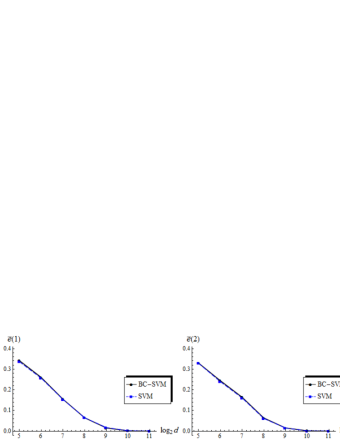
(a) $(n_{1},n_{2})=(10,10)$ and $\mbox{\boldmath$\Sigma$}_{1}=\mbox{\boldmath$\Sigma$}_{2}=\mbox{\boldmath{$I$}}_{d}$ (i.e., $\kappa=0$)

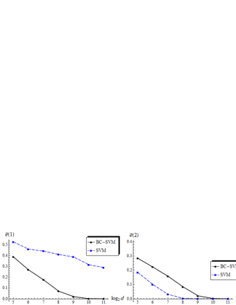
(b) $(n_{1},n_{2})=(6,14)$ and $\mbox{\boldmath$\Sigma$}_{1}=\mbox{\boldmath$\Sigma$}_{2}=\mbox{\boldmath{$I$}}_{d}$ (i.e., $\kappa/\Delta=6/7$)

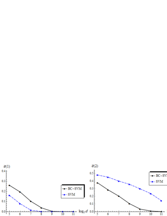
(c) $(n_{1},n_{2})=(10,10)$, $\mbox{\boldmath$\Sigma$}_{1}=0.6\mbox{\boldmath{$I$}}_{d}$ and $\mbox{\boldmath$\Sigma$}_{2}=1.4\mbox{\boldmath{$I$}}_{d}$ (i.e., $\kappa/\Delta=-18/25$)

Figure 2: The performance of the BC-SVM in HDLSS settings. The error rates are denoted by the solid lines for (a), (b) and (c). The left panels display $\overline{e}(1)$, the middle panels display $\overline{e}(2)$ and the right panels display $\overline{e}$. The corresponding error rates by the SVM are denoted by the dashed lines. Their standard deviations are less than $0.0112$.

Next, we compared the performance of the BC-SVM with the SVM in complex settings. We set $\mbox{\boldmath$\mu$}_{1}=\mbox{\boldmath{$0$}}$, $\mbox{\boldmath$\Sigma$}_{1}=\mbox{\boldmath{$B$}}(0.3^{|i-j|^{1/3}})\mbox{\boldmath{$B$}}$ and $\mbox{\boldmath$\Sigma$}_{2}=\mbox{\boldmath{$B$}}(0.4^{|i-j|^{1/3}})\mbox{\boldmath{$B$}}$, where

$$\mbox{\boldmath{$B$}}=\mbox{diag}[\{0.5+1/(d+1)\}^{1/2},...,\{0.5+d/(d+1)\}^{1/2}].$$

Note that $\mbox{\rm tr}(\mbox{\boldmath$\Sigma$}_{1})=\mbox{\rm tr}(\mbox{\boldmath$\Sigma$}_{2})=d$. We considered two cases:

$\mbox{\boldmath$\mu$}_{2}=(1,...,1,0,...,0,-1,...,-1)^{T}$ $(=\mbox{\boldmath$\mu$}_{\alpha}(t),\ \mbox{say})$ whose first $t/2$ elements are $1$ and last $t/2$ elements are $-1$ for a positive even number $t$; and

$\mbox{\boldmath$\mu$}_{2}=(t^{1/2}/2,t^{1/2}/2,0,...,0,-t^{1/2}/2,-t^{1/2}/2)^{T}$ $(=\mbox{\boldmath$\mu$}_{\beta}(t),\ \mbox{say})$ whose first two elements are $t^{1/2}/2$ and last two elements are $-t^{1/2}/2$ for a positive number $t$.

Note that $\Delta=t$ both for $\mbox{\boldmath$\mu$}_{\alpha}(t)$ and $\mbox{\boldmath$\mu$}_{\beta}(t)$. We generated $\mbox{\boldmath{$x$}}_{ij}-\mbox{\boldmath$\mu$}_{i}$, $i=1,2;\ j=1,2,...,$ independently either from (I) $N_{d}(\mbox{\boldmath{$0$}},\mbox{\boldmath$\Sigma$}_{i}),\ i=1,2$, or (II) a $d$-variate $t$-distribution, $t_{d}(\mbox{\boldmath$\Sigma$}_{i},10),\ i=1,2$, with mean zero, covariance matrix $\mbox{\boldmath$\Sigma$}_{i}$ and degrees of freedom 10. Note that (A-i) holds under (A-ii) for (I). Let $d_{*}=2\lceil d^{2/3}/2\rceil$, where $\lceil x\rceil$ denotes the smallest integer $\geq x$. We considered four cases:

(d) $\mbox{\boldmath$\mu$}_{2}=\mbox{\boldmath$\mu$}_{\alpha}(d_{*})$, $(n_{1},n_{2})=(5,25)$ and $d=2^{s},\ s=6,...,12$, for (I);

(e) $\mbox{\boldmath$\mu$}_{2}=\mbox{\boldmath$\mu$}_{\alpha}(d_{*})$, $d=1000$ and $(n_{1},n_{2})=(4s,8s),\ s=1,...,7$, for (II);

(f) $d=1000$, $(n_{1},n_{2})=(10,20)$ and $\mbox{\boldmath$\mu$}_{2}=\mbox{\boldmath$\mu$}_{\alpha}(2^{s}),\ s=1,...,7$, for (II); and

(g) $d=1000$, $(n_{1},n_{2})=(10,20)$ and $\mbox{\boldmath$\mu$}_{2}=\mbox{\boldmath$\mu$}_{\beta}(2^{s}),\ s=1,...,7$, for (II).

Note that $\Delta=d_{*}=o(d)$ and (A-ii) holds for (d) and (e) from the fact that $\mbox{\rm tr}(\mbox{\boldmath$\Sigma$}_{i}^{2})=O(d)$, $i=1,2$. Also, note that (A-i) holds for (d). However, (A-i) does not hold for (e) and (A-iii) does not hold both for (d) and (e). For (f) and (g), we note that $\Delta=2^{s},\ s=1,...,7$. Especially, (g) is a sparse case such that the only four elements of $\mbox{\boldmath$\mu$}_{1}-\mbox{\boldmath$\mu$}_{2}$ are nonzero. Similar to Section 1, we calculated the error rates, $\overline{e}(1)$, $\overline{e}(2)$ and $\overline{e}$, by 2000 replications and plotted the results in Figure 3.

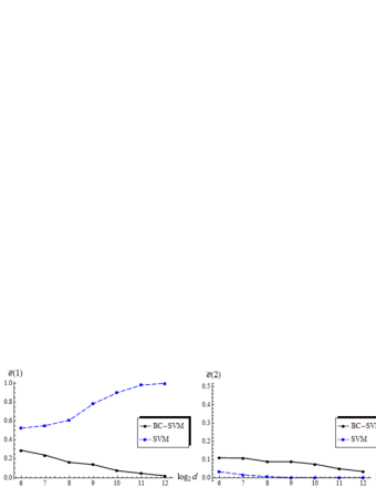
(d) $\mbox{\boldmath$\mu$}_{2}=\mbox{\boldmath$\mu$}_{\alpha}(d_{*})$ $(\Delta\approx d^{2/3})$, $(n_{1},n_{2})=(5,25)$ and $d=2^{s},\ s=6,...,12$, for (I) $N_{d}(\mbox{\boldmath{$0$}},\mbox{\boldmath$\Sigma$}_{i})$

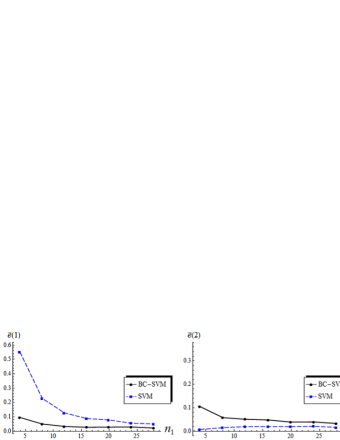
(e) $\mbox{\boldmath$\mu$}_{2}=\mbox{\boldmath$\mu$}_{\alpha}(d_{*})$ $(\Delta\approx d^{2/3})$, $d=1000$ and $(n_{1},n_{2})=(4s,8s),\ s=1,...,7$, for (II) $t_{d}(\mbox{\boldmath$\Sigma$}_{i},10)$

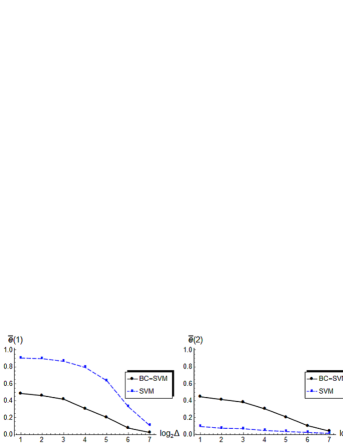
(f) $d=1000$, $(n_{1},n_{2})=(10,20)$ and $\mbox{\boldmath$\mu$}_{2}=\mbox{\boldmath$\mu$}_{\alpha}(2^{s})\ (\Delta=2^{s}),\ s=1,...,7$, for (II) $t_{d}(\mbox{\boldmath$\Sigma$}_{i},10)$

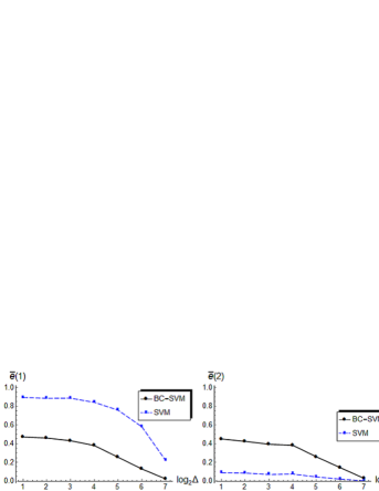
(g) $d=1000$, $(n_{1},n_{2})=(10,20)$ and $\mbox{\boldmath$\mu$}_{2}=\mbox{\boldmath$\mu$}_{\beta}(2^{s})\ (\Delta=2^{s}),\ s=1,...,7$, for (II) $t_{d}(\mbox{\boldmath$\Sigma$}_{i},10)$

Figure 3: The error rates of the BC-SVM and the SVM are denoted by the solid lines and the dashed lines, respectively, for (d) to (g). The left panels display $\overline{e}(1)$, the middle panels display $\overline{e}(2)$ and the right panels display $\overline{e}$. Their standard deviations are less than $0.0112$.

We observe that the SVM gives quite bad performances for (d) in Figure 3. The main reason must be due to the bias term in the SVM. Note that $\kappa/\Delta\to\infty$ as $d\to\infty$ for (d). Thus $\overline{e}(1)$ becomes close to $1$ as $d$ increases. See Corollary 1 for the details. Also, the SVM gives bad performances for (e) to (g) when $n_{i}$s are small or $\Delta$ is small. This is because $\kappa/\Delta$ becomes large when $n_{i}$s are small or $\Delta$ is small. On the other hand, from Figures 2 and 3, the BC-SVM gives adequate performances even when $n_{i}$s and $\mbox{\boldmath$\Sigma$}_{i}$s are unbalanced. The BC-SVM also gives a better performance than the SVM even when $\Delta$ is small (or sparse).

4.2 Examples: Microarray data sets

First, we used colon cancer data with $2000\ (=d)$ genes given by Alon et al. (1999) which consists of $\pi_{1}:$ colon tumor (40 samples) and $\pi_{2}:$ normal colon (22 samples). We set $n_{1}=n_{2}=10$. We randomly split the data sets from $(\pi_{1},\pi_{2})$ into training data sets of sizes $(n_{1},n_{2})$ and test data sets of sizes $(40-n_{1},22-n_{2})$. We constructed the BC-SVM and the SVM by using the training data sets. We checked accuracy by using the test data set for each $\pi_{i}$ and denoted the misclassification rates by $\widehat{e}(1)_{r}$ and $\widehat{e}(2)_{r}$. We repeated this procedure 100 times and obtained $\widehat{e}(1)_{r}$ and $\widehat{e}(2)_{r}$, $r=1,...,100$, both for the BC-SVM and the SVM. We had the average misclassification rates as $\overline{e}(1)\ (=\sum_{r=1}^{100}\widehat{e}(1)_{r}/100)=0.16$, $\overline{e}(2)\ (=\sum_{r=1}^{100}\widehat{e}(2)_{r}/100)=0.166$ and $\overline{e}\ (=\{\overline{e}(1)+\overline{e}(2)\}/2)=0.163$ for the BC-SVM, and $\overline{e}(1)=0.158$, $\overline{e}(2)=0.161$ and $\overline{e}=0.159$ for the SVM. By using all the samples, we considered estimating $\kappa/\Delta$. We set $m_{1}=40$ and $m_{2}=22$. From Section 3.1 in Aoshima and Yata (2011), an unbiased estimator of $\Delta$ was given by $\hat{\Delta}_{(m)}=\|\overline{\mbox{\boldmath{$x$}}}_{1m_{1}}-\overline{\mbox{\boldmath{$x$}}}_{2m_{2}}\|^{2}-\mbox{\rm tr}(\mbox{\boldmath{$S$}}_{1m_{1}})/m_{1}-\mbox{\rm tr}(\mbox{\boldmath{$S$}}_{2m_{2}})/m_{2}$. We estimated $\kappa/\Delta$ by

$$\widehat{\kappa/\Delta}=\{\mbox{\rm tr}(\mbox{\boldmath{$S$}}_{1m_{1}})/n_{1}-\mbox{\rm tr}(\mbox{\boldmath{$S$}}_{2m_{2}})/n_{2}\}/\hat{\Delta}_{(m)}$$

and had $\widehat{\kappa/\Delta}=0.003$ for the $62$ samples. In view of (9), we expect that the BC-SVM is asymptotically equivalent to the SVM in such cases. We estimated $(\mbox{\rm tr}(\mbox{\boldmath$\Sigma$}_{1})/\Delta,\mbox{\rm tr}(\mbox{\boldmath$\Sigma$}_{2})/\Delta)$ by $(\mbox{\rm tr}(\mbox{\boldmath{$S$}}_{1m_{1}})/\hat{\Delta}_{(m)},\mbox{\rm tr}(\mbox{\boldmath{$S$}}_{2m_{2}})/\hat{\Delta}_{(m)})=(3.99,3.959)$. It is difficult to estimate the standard deviation of the average misclassification rate. However, by noting that $\mbox{\rm Var}\{\overline{e}(i)\}^{1/2}<\mbox{\rm Var}\{\widehat{e}(i)_{r}\}^{1/2}=[e(i)\{1-e(i)\}/(m_{i}-n_{i})]^{1/2}$, one may have an upper bound of the standard deviation for $\overline{e}(i)$ as

$$s_{u}(i)=[\overline{e}(i)\{1-\overline{e}(i)\}/(m_{i}-n_{i})]^{1/2},$$

so that $\{\sum_{i=1}^{2}s_{u}(i)^{2}/2\}^{1/2}\ (=s_{u},$ $\mbox{say})$ for $\overline{e}$. For the BC-SVM, $s_{u}(1)=0.067$, $s_{u}(2)=0.107$ and $s_{u}=0.089$. We summarized the results for various $n_{i}$s in Table 1.

Table 1: Average misclassification rates of the BC-SVM and the SVM, together with $\widehat{\kappa/\Delta}$, for Alon et al. (1999)’s colon cancer data ($d=2000$, $m_{1}=40$ and $m_{2}=22$). For each case, the standard deviations of $\overline{e}(1)$, $\overline{e}(2)$ and $\overline{e}$ are less than $s_{u}(1)$, $s_{u}(2)$ and $s_{u}$, respectively.

	BC-SVM			SVM
$(n_{1},n_{2})$	$\overline{e}(1)$	$\overline{e}(2)$	$\overline{e}$	$\overline{e}(1)$	$\overline{e}(2)$	$\overline{e}$	$\widehat{\kappa/\Delta}$
$(10,5)$	$0.188$	$0.209$	$0.198$	$0.122$	$0.309$	$0.215$	$-0.393$
$(10,10)$	$0.16$	$0.166$	$0.163$	$0.158$	$0.161$	$0.159$	$0.003$
$(10,15)$	$0.184$	$0.156$	$0.17$	$0.206$	$0.134$	$0.17$	$0.135$
$(20,5)$	$0.164$	$0.249$	$0.206$	$0.082$	$0.475$	$0.278$	$-0.592$
$(20,10)$	$0.141$	$0.177$	$0.159$	$0.116$	$0.23$	$0.173$	$-0.196$
$(20,15)$	$0.142$	$0.167$	$0.154$	$0.133$	$0.181$	$0.157$	$-0.064$
$(30,5)$	$0.144$	$0.302$	$0.223$	$0.083$	$0.566$	$0.324$	$-0.659$
$(30,10)$	$0.12$	$0.236$	$0.178$	$0.108$	$0.318$	$0.213$	$-0.263$
$(30,15)$	$0.115$	$0.203$	$0.159$	$0.1$	$0.263$	$0.181$	$-0.131$

Next, we used leukemia data with $7129\ (=d)$ genes given by Golub et al. (1999) which consists of $\pi_{1}:$ ALL (47 $(=m_{1})$ samples) and $\pi_{2}:$ AML (25 $(=m_{2})$ samples). We applied the BC-SVM and the SVM to the leukemia data and summarized the results in Table 2. When $n_{1}\neq n_{2}$, $|\widehat{\kappa/\Delta}|$ becomes large since $(\mbox{\rm tr}(\mbox{\boldmath{$S$}}_{1m_{1}})/\hat{\Delta}_{(m)},\mbox{\rm tr}(\mbox{\boldmath{$S$}}_{2m_{2}})/\hat{\Delta}_{(m)})=(2.693,2.785)$. As expected theoretically, we observe that the BC-SVM gives adequate performances compared to the SVM when $|\widehat{\kappa/\Delta}|$ is not small.

Table 2: Average misclassification rates of the BC-SVM and the SVM, together with $\widehat{\kappa/\Delta}$, for Golub et al. (1999)’s leukemia data ($d=7129$, $m_{1}=47$ and $m_{2}=25$). For each case, the standard deviations of $\overline{e}(1)$, $\overline{e}(2)$ and $\overline{e}$ are less than $s_{u}(1)$, $s_{u}(2)$ and $s_{u}$, respectively.

	BC-SVM			SVM
$(n_{1},n_{2})$	$\overline{e}(1)$	$\overline{e}(2)$	$\overline{e}$	$\overline{e}(1)$	$\overline{e}(2)$	$\overline{e}$	$\widehat{\kappa/\Delta}$
$(10,5)$	$0.044$	$0.077$	$0.06$	$0.012$	$0.148$	$0.08$	$-0.288$
$(10,10)$	$0.036$	$0.043$	$0.04$	$0.036$	$0.046$	$0.041$	$-0.009$
$(10,20)$	$0.044$	$0.034$	$0.039$	$0.074$	$0.026$	$0.05$	$0.13$
$(20,5)$	$0.031$	$0.067$	$0.049$	$0.004$	$0.199$	$0.102$	$-0.422$
$(20,10)$	$0.019$	$0.051$	$0.035$	$0.011$	$0.071$	$0.041$	$-0.144$
$(20,20)$	$0.028$	$0.046$	$0.037$	$0.028$	$0.046$	$0.037$	$-0.005$
$(40,5)$	$0.017$	$0.102$	$0.059$	$0.0$	$0.297$	$0.149$	$-0.49$
$(40,10)$	$0.016$	$0.047$	$0.031$	$0.003$	$0.091$	$0.047$	$-0.211$
$(40,20)$	$0.011$	$0.03$	$0.021$	$0.006$	$0.032$	$0.019$	$-0.072$

Finally, we used myeloma data with $12625\ (=d)$ genes given by Tian et al. (2003) which consists of $\pi_{1}:$ patients without bone lesions (36 $(=m_{1})$ samples) and $\pi_{2}:$ patients with bone lesions (137 $(=m_{2})$ samples). We applied the BC-SVM and the SVM to the myeloma data and summarized the results in Table 3. When $n_{1}$ and $n_{2}$ are unbalanced, the SVM gives a very bad performance. This is because $\Delta$ in such cases is not sufficiently large since $(\mbox{\rm tr}(\mbox{\boldmath$\Sigma$}_{1})/\Delta,\mbox{\rm tr}(\mbox{\boldmath$\Sigma$}_{2})/\Delta)\approx(\mbox{\rm tr}(\mbox{\boldmath{$S$}}_{1m_{1}})/\hat{\Delta}_{(m)},\mbox{\rm tr}(\mbox{\boldmath{$S$}}_{2m_{2}})/\hat{\Delta}_{(m)})=(33.69,33.53)$, so that $\kappa/\Delta$ becomes too large when $n_{1}\neq n_{2}$. Especially when $\widehat{\kappa/\Delta}>1$, $\overline{e}(1)$ of the SVM is too large. See Corollary 1 for the details. The BC-SVM also does not give a low error rate for this data because $\Delta$ is not sufficiently large. However, the BC-SVM gives adequate performances compared to the SVM especially when $\widehat{\kappa/\Delta}>1$. Throughout Sections 3 and 4, we recommend to use the BC-SVM rather than the SVM for high-dimensional data.

Table 3: Average misclassification rates of the BC-SVM and the SVM, together with $\widehat{\kappa/\Delta}$, for Tian et al. (2003)’s myeloma data ($d=12625$, $m_{1}=36$ and $m_{2}=137$). For each case, the standard deviations of $\overline{e}(1)$, $\overline{e}(2)$ and $\overline{e}$ are less than $s_{u}(1)$, $s_{u}(2)$ and $s_{u}$, respectively.

	BC-SVM			SVM
$(n_{1},n_{2})$	$\overline{e}(1)$	$\overline{e}(2)$	$\overline{e}$	$\overline{e}(1)$	$\overline{e}(2)$	$\overline{e}$	$\widehat{\kappa/\Delta}$
$(10,25)$	$0.367$	$0.307$	$0.337$	$0.787$	$0.059$	$0.423$	$2.028$
$(10,50)$	$0.407$	$0.265$	$0.336$	$0.936$	$0.013$	$0.475$	$2.698$
$(10,100)$	$0.501$	$0.193$	$0.347$	$0.993$	$0.003$	$0.498$	$3.034$
$(20,25)$	$0.311$	$0.288$	$0.299$	$0.401$	$0.214$	$0.308$	$0.343$
$(20,50)$	$0.343$	$0.25$	$0.296$	$0.646$	$0.085$	$0.365$	$1.014$
$(20,100)$	$0.436$	$0.175$	$0.306$	$0.872$	$0.026$	$0.449$	$1.349$
$(30,25)$	$0.303$	$0.288$	$0.296$	$0.25$	$0.341$	$0.295$	$-0.218$
$(30,50)$	$0.33$	$0.26$	$0.295$	$0.467$	$0.162$	$0.314$	$0.452$
$(30,100)$	$0.382$	$0.195$	$0.288$	$0.713$	$0.068$	$0.391$	$0.788$

5 Multiclass SVMs

In this section, we consider multiclass SVMs in HDLSS settings. We have i.i.d. observations, $\mbox{\boldmath{$x$}}_{i1},...,\mbox{\boldmath{$x$}}_{in_{i}}$, from each $\pi_{i}\ (i=1,...,g)$, where $g\geq 3$ and $\pi_{i}$ has a $d$-dimensional distribution with an unknown mean vector $\mbox{\boldmath$\mu$}_{i}$ and unknown covariance matrix $\mbox{\boldmath$\Sigma$}_{i}\ (\geq\mbox{\boldmath{$O$}})$. We assume $n_{i}\geq 2,\ i=1,...,g$. Let $\Delta_{ij}=\|\mbox{\boldmath$\mu$}_{i}-\mbox{\boldmath$\mu$}_{j}\|^{2}$ for $i,j=1,...,g;\ i\neq j$. We assume that $\mbox{\rm tr}(\mbox{\boldmath$\Sigma$}_{i})/d\in(0,\infty)$ as $d\to\infty$ for $i=1,...,g$, and $\limsup_{d\to\infty}\Delta_{ij}/d<\infty$ for $i,j=1,...,g;\ i\neq j$. We consider the one-versus-one approach (the max-wins rule). See Friedman (1996) and Bishop (2006) for the details. Let $N_{g}=\sum_{i=1}^{g}n_{i}$. First, we consider the case when $d\to\infty$ while $N_{g}$ is fixed. We consider the following assumptions:

(B-i)

$\displaystyle\frac{\max_{l=i,j}\mbox{\rm Var}(\|\mbox{\boldmath{$x$}}_{lk}-\mbox{\boldmath$\mu$}_{l}\|^{2})}{\Delta_{ij}^{2}}\to 0$ as $d\to\infty$ for $i,j=1,...,g;\ i\neq j$;

(B-ii)

$\displaystyle\frac{\max_{l=i,j}\mbox{\rm tr}(\mbox{\boldmath$\Sigma$}_{l}^{2})}{\Delta_{ij}^{2}}\to 0$ as $d\to\infty$ for $i,j=1,...,g;\ i\neq j$.

Let $\kappa_{ij}=\mbox{\rm tr}(\mbox{\boldmath$\Sigma$}_{i})/n_{i}-\mbox{\rm tr}(\mbox{\boldmath$\Sigma$}_{j})/n_{j}$ for $i,j=1,...,g;\ i\neq j$. We consider the following condition:

(B-iii)

$\displaystyle\limsup_{d\to\infty}\frac{|\kappa_{ij}|}{\Delta_{ij}}<1$ for $i,j=1,...,g;\ i\neq j$.

From Theorem 1, for the one-versus-one approach by (5), we have the following result.

Corollary 4.

Under (B-i) to (B-iii), it holds for the multiclass SVM that

$$e(i)\to 0\ \ \mbox{as $d\to\infty$ for $i=1,...,g$}.$$ (11)

From Theorem 2, for the one-versus-one approach by (9), we have the following result.

Corollary 5.

Under (B-i) and (B-ii), the multiclass BC-SVM holds (11).

Note that the BC-SVM satisfies the consistency property without (B-iii). Thus we recommend to use the BC-SVM in multiclass HDLSS settings.

Next, we consider the case when both $d,N_{g}\to\infty$ while $N_{g}/d\to 0$. Similar to Section 2.3 and Corollary 3, the multiclass SVMs have the consistency property under some regularity conditions.

We checked the performance of the multiclass SVMs by using leukemia data with $12582\ (=d)$ genes given by Armstrong et al. (2002) which consists of $\pi_{1}:$ ALL (24 $(=m_{1})$ samples), $\pi_{2}:$ MLL (20 $(=m_{2})$ samples) and $\pi_{3}:$ AML (28 $(=m_{3})$ samples). We applied the multiclass BC-SVM and SVM to the leukemia and summarized the results in Table 4. We had $(\mbox{\rm tr}(\mbox{\boldmath{$S$}}_{1m_{1}})/\hat{\Delta}_{12(m)},$ $\mbox{\rm tr}(\mbox{\boldmath{$S$}}_{2m_{2}})/\hat{\Delta}_{12(m)})=(2.724,3.213)$, $(\mbox{\rm tr}(\mbox{\boldmath{$S$}}_{1m_{1}})/\hat{\Delta}_{13(m)},\mbox{\rm tr}(\mbox{\boldmath{$S$}}_{3m_{3}})/\hat{\Delta}_{13(m)})=(0.738,0.9)$ and $(\mbox{\rm tr}(\mbox{\boldmath{$S$}}_{2m_{2}})/\hat{\Delta}_{23(m)},\mbox{\rm tr}(\mbox{\boldmath{$S$}}_{3m_{3}})/\hat{\Delta}_{23(m)})=(1.533,1.585)$, where $\hat{\Delta}_{ij(m)}=\|\overline{\mbox{\boldmath{$x$}}}_{im_{i}}-\overline{\mbox{\boldmath{$x$}}}_{jm_{j}}\|^{2}-\mbox{\rm tr}(\mbox{\boldmath{$S$}}_{im_{i}})/m_{i}-\mbox{\rm tr}(\mbox{\boldmath{$S$}}_{jm_{j}})/m_{j}$ that is an unbiased estimator of $\Delta_{ij}$. Thus $|\kappa_{ij}/\Delta_{ij}|$ must become large when $n_{i}\neq n_{j}$. Actually, the multiclass BC-SVM gives adequate performances for all the cases.

Table 4: Average misclassification rates of the BC-SVM and the SVM for Armstrong et al. (2002)’s leukemia data ($d=12582$, $m_{1}=24$, $m_{2}=20$ and $m_{3}=28$). For each case, the standard deviations of $\overline{e}(i)$, $i=1,2,3,$ and $\overline{e}$ are less than $s_{u}(i)$, $i=1,2,3,$ and $s_{u}=\{\sum_{i=1}^{3}s_{u}(i)^{2}/3\}^{1/2}$, respectively.

	BC-SVM				SVM
$(n_{1},n_{2},n_{3})$	$\overline{e}(1)$	$\overline{e}(2)$	$\overline{e}(3)$	$\overline{e}$	$\overline{e}(1)$	$\overline{e}(2)$	$\overline{e}(3)$	$\overline{e}$
$(5,5,10)$	$0.085$	$0.089$	$0.071$	$0.082$	$0.069$	$0.118$	$0.06$	$0.082$
$(5,5,20)$	$0.103$	$0.087$	$0.07$	$0.087$	$0.089$	$0.135$	$0.053$	$0.092$
$(5,10,10)$	$0.049$	$0.06$	$0.066$	$0.058$	$0.095$	$0.047$	$0.066$	$0.069$
$(5,10,20)$	$0.044$	$0.068$	$0.064$	$0.059$	$0.088$	$0.06$	$0.06$	$0.069$
$(10,5,10)$	$0.051$	$0.077$	$0.063$	$0.064$	$0.021$	$0.143$	$0.049$	$0.071$
$(10,5,20)$	$0.051$	$0.073$	$0.061$	$0.062$	$0.018$	$0.148$	$0.044$	$0.07$
$(10,10,10)$	$0.028$	$0.056$	$0.063$	$0.049$	$0.025$	$0.059$	$0.064$	$0.049$
$(10,10,20)$	$0.031$	$0.051$	$0.071$	$0.051$	$0.03$	$0.058$	$0.065$	$0.051$

Appendix A

Throughout, let $\mbox{\boldmath$\mu$}=\mbox{\boldmath$\mu$}_{1}-\mbox{\boldmath$\mu$}_{2}$ and $\mbox{\boldmath$\mu$}_{*}=(\mbox{\boldmath$\mu$}_{1}+\mbox{\boldmath$\mu$}_{2})/2$.

Proof of Lemma 1.

Under (A-ii), we have that as $d\to\infty$

$$\mbox{\boldmath$\mu$}^{T}\mbox{\boldmath$\Sigma$}_{i}\mbox{\boldmath$\mu$}/\Delta^{2}\leq\mbox{\rm tr}(\mbox{\boldmath$\Sigma$}_{i}^{2})^{1/2}/\Delta=o(1),\quad i=1,2.$$ (12)

Then, by using Chebyshev’s inequality, for any $\tau>0$, under (A-ii), we have that

$$P(|(\mbox{\boldmath{$x$}}_{j}-\mbox{\boldmath$\mu$}_{*})^{T}(\mbox{\boldmath{$x$}}_{k}-\mbox{\boldmath$\mu$}_{*})-\Delta/4|\geq\tau\Delta)$$

$$\leq(\tau\Delta)^{-2}E[\{(\mbox{\boldmath{$x$}}_{j}-\mbox{\boldmath$\mu$}_{*})^{T}(\mbox{\boldmath{$x$}}_{k}-\mbox{\boldmath$\mu$}_{*})-\Delta/4\}^{2}]$$

$$=O\{\mbox{\rm tr}(\mbox{\boldmath$\Sigma$}_{1}^{2})+\mbox{\boldmath$\mu$}^{T}\mbox{\boldmath$\Sigma$}_{1}\mbox{\boldmath$\mu$}\}/\Delta^{2}=o(1)\quad\mbox{for $1\leq j<k\leq n_{1}$};$$

$$P(|(\mbox{\boldmath{$x$}}_{j}-\mbox{\boldmath$\mu$}_{*})^{T}(\mbox{\boldmath{$x$}}_{k}-\mbox{\boldmath$\mu$}_{*})-\Delta/4|\geq\tau\Delta)$$

$$=O\{\mbox{\rm tr}(\mbox{\boldmath$\Sigma$}_{2}^{2})+\mbox{\boldmath$\mu$}^{T}\mbox{\boldmath$\Sigma$}_{2}\mbox{\boldmath$\mu$}\}/\Delta^{2}=o(1)\quad\mbox{for $n_{1}+1\leq j<k\leq N$};\quad\mbox{and}$$

$$P(|(\mbox{\boldmath{$x$}}_{j}-\mbox{\boldmath$\mu$}_{*})^{T}(\mbox{\boldmath{$x$}}_{k}-\mbox{\boldmath$\mu$}_{*})+\Delta/4|\geq\tau\Delta)$$

$$=O\{\mbox{\rm tr}(\mbox{\boldmath$\Sigma$}_{1}\mbox{\boldmath$\Sigma$}_{2})+\mbox{\boldmath$\mu$}^{T}(\mbox{\boldmath$\Sigma$}_{1}+\mbox{\boldmath$\Sigma$}_{2})\mbox{\boldmath$\mu$}\}/\Delta^{2}=o(1)$$

for $$1\leq j\leq n_{1} n_{1}+1\leq k\leq N$$ and (13)

from the fact that $\mbox{\rm tr}(\mbox{\boldmath$\Sigma$}_{1}\mbox{\boldmath$\Sigma$}_{2})\leq\{\mbox{\rm tr}(\mbox{\boldmath$\Sigma$}_{1}^{2})\mbox{\rm tr}(\mbox{\boldmath$\Sigma$}_{2}^{2})\}^{1/2}$. From (12), for any $\tau>0$, we have that

$$P(|\|\mbox{\boldmath{$x$}}_{j}-\mbox{\boldmath$\mu$}_{*}\|^{2}-\Delta/4-\mbox{\rm tr}(\mbox{\boldmath$\Sigma$}_{1})|\geq\tau\Delta)$$

$$=O\{\mbox{Var}(\|\mbox{\boldmath{$x$}}_{1j}-\mbox{\boldmath$\mu$}_{1}\|^{2})+\mbox{\boldmath$\mu$}^{T}\mbox{\boldmath$\Sigma$}_{1}\mbox{\boldmath$\mu$}\}/\Delta^{2}=o(1)\quad\mbox{for $j=1,...,n_{1}$};\quad and$$

$$P(|\|\mbox{\boldmath{$x$}}_{j}-\mbox{\boldmath$\mu$}_{*}\|^{2}-\Delta/4-\mbox{\rm tr}(\mbox{\boldmath$\Sigma$}_{2})|\geq\tau\Delta)=o(1)\quad\mbox{for $j=n_{1}+1,...,N$}$$ (14)

under (A-i) and (A-ii). Here, subject to (4), we can write for (3) that

$$L(\mbox{\boldmath$\alpha$})=\sum_{j=1}^{N}\alpha_{j}-\frac{1}{2}\sum_{j=1}^{N}\sum_{k=1}^{N}\alpha_{j}\alpha_{k}t_{j}t_{k}(\mbox{\boldmath{$x$}}_{j}-\mbox{\boldmath$\mu$}_{*})^{T}(\mbox{\boldmath{$x$}}_{k}-\mbox{\boldmath$\mu$}_{*}).$$ (15)

Then, by noting that $\alpha_{j}\geq 0$ for all $j$ subject to (4), from (13) and (14), we have that

$$L(\mbox{\boldmath$\alpha$})= \sum_{j=1}^{N}\alpha_{j}-\frac{\Delta}{8}\Big{(}\sum_{j=1}^{N}\alpha_{j}\Big{)}^{2}-\frac{1}{2}\Big{(}\mbox{\rm tr}(\mbox{\boldmath$\Sigma$}_{1})\sum_{j=1}^{n_{1}}\alpha_{j}^{2}+\mbox{\rm tr}(\mbox{\boldmath$\Sigma$}_{2})\sum_{j=n_{1}+1}^{N}\alpha_{j}^{2}\Big{)}$$

$$+o_{p}\Big{\{}\Delta\Big{(}\sum_{j=1}^{N}\alpha_{j}\Big{)}^{2}\Big{\}}$$ (16)

subject to (4) under (A-i) and (A-ii). It concludes the result. ∎

Proof of Lemma 2.

By combining Lemma 1 with (6) and (7), we can claim the first result.

When $\hat{S}=\{1,...,N\}$, by noting that $\sum_{j=1}^{N}\hat{\alpha}_{j}t_{j}=0$, we have that

$$\hat{y}(\mbox{\boldmath{$x$}}_{0})= \sum_{j=1}^{N}\hat{\alpha}_{j}t_{j}(\mbox{\boldmath{$x$}}_{j}-\mbox{\boldmath$\mu$}_{*})^{T}(\mbox{\boldmath{$x$}}_{0}-\mbox{\boldmath$\mu$}_{*})+\sum_{j=1}^{N}\hat{\alpha}_{j}t_{j}(\mbox{\boldmath{$x$}}_{j}-\mbox{\boldmath$\mu$}_{*})^{T}\mbox{\boldmath$\mu$}_{*}+\hat{b}$$

$$= \sum_{j=1}^{N}\hat{\alpha}_{j}t_{j}(\mbox{\boldmath{$x$}}_{j}-\mbox{\boldmath$\mu$}_{*})^{T}(\mbox{\boldmath{$x$}}_{0}-\mbox{\boldmath$\mu$}_{*})$$

$$+\frac{-n_{1}+n_{2}}{N}-\frac{1}{N}\sum_{j=1}^{N}\sum_{k=1}^{N}\hat{\alpha}_{k}t_{k}(\mbox{\boldmath{$x$}}_{j}-\mbox{\boldmath$\mu$}_{*})^{T}(\mbox{\boldmath{$x$}}_{k}-\mbox{\boldmath$\mu$}_{*}).$$ (17)

From the first result of Lemma 2, (13) and (14), we have that as $d\to\infty$

$$\frac{-n_{1}+n_{2}}{N}-\frac{1}{N}\sum_{j=1}^{N}\sum_{k=1}^{N}\hat{\alpha}_{k}t_{k}(\mbox{\boldmath{$x$}}_{j}-\mbox{\boldmath$\mu$}_{*})^{T}(\mbox{\boldmath{$x$}}_{k}-\mbox{\boldmath$\mu$}_{*})$$

$$=\frac{-n_{1}+n_{2}}{N}+\frac{(n_{1}-n_{2})\Delta}{\Delta_{*}N}+2\frac{\mbox{\rm tr}(\mbox{\boldmath$\Sigma$}_{1})-\mbox{\rm tr}(\mbox{\boldmath$\Sigma$}_{2})}{\Delta_{*}N}+o_{p}\Big{(}\frac{\Delta}{\Delta_{*}}\Big{)}$$

$$=\frac{-n_{1}+n_{2}}{N}\Big{(}\frac{\delta}{\Delta_{*}}\Big{)}+2\frac{\mbox{\rm tr}(\mbox{\boldmath$\Sigma$}_{1})-\mbox{\rm tr}(\mbox{\boldmath$\Sigma$}_{2})}{\Delta_{*}N}+o_{p}\Big{(}\frac{\Delta}{\Delta_{*}}\Big{)}$$

$$=\frac{\mbox{\rm tr}(\mbox{\boldmath$\Sigma$}_{1})/n_{1}-\mbox{\rm tr}(\mbox{\boldmath$\Sigma$}_{2})/n_{2}}{\Delta_{*}}+o_{p}\Big{(}\frac{\Delta}{\Delta_{*}}\Big{)}$$ (18)

under (A-i) and (A-ii). Similar to (13), under (A-ii), we obtain that $(\mbox{\boldmath{$x$}}_{j}-\mbox{\boldmath$\mu$}_{*})^{T}(\mbox{\boldmath{$x$}}_{0}-\mbox{\boldmath$\mu$}_{*})/\Delta=(-1)^{i+1}/4+o_{p}(1)$ for $j=1,...,n_{1}$, and $(\mbox{\boldmath{$x$}}_{j}-\mbox{\boldmath$\mu$}_{*})^{T}(\mbox{\boldmath{$x$}}_{0}-\mbox{\boldmath$\mu$}_{*})/\Delta=(-1)^{i}/4+o_{p}(1)$ for $j=n_{1}+1,...,N$, when $\mbox{\boldmath{$x$}}_{0}\in\pi_{i}$ $(i=1,2)$. Then, from the first result of Lemma 2, under (A-i) and (A-ii), it holds that

$$\sum_{j=1}^{N}\hat{\alpha}_{j}t_{j}(\mbox{\boldmath{$x$}}_{j}-\mbox{\boldmath$\mu$}_{*})^{T}(\mbox{\boldmath{$x$}}_{0}-\mbox{\boldmath$\mu$}_{*})=\frac{(-1)^{i}\Delta}{\Delta_{*}}+o_{p}\Big{(}\frac{\Delta}{\Delta_{*}}\Big{)}$$ (19)

when $\mbox{\boldmath{$x$}}_{0}\in\pi_{i}$ for $i=1,2$. By combining (17) with (18) and (19), we can conclude the second result. ∎

Proofs of Theorem 1 and Corollary 1.

By using (8), the results are obtained straightforwardly. ∎

Proof of Lemma 3.

Similar to (13), under (A-ii’), from (12), we have that as $d,N\to\infty$

$$\sum_{1\leq j<k\leq n_{1}}P(|(\mbox{\boldmath{$x$}}_{j}-\mbox{\boldmath$\mu$}_{1})^{T}(\mbox{\boldmath{$x$}}_{k}-\mbox{\boldmath$\mu$}_{1})|\geq\tau\Delta)=O\Big{(}\frac{n_{1}^{2}\mbox{\rm tr}(\mbox{\boldmath$\Sigma$}_{1}^{2})}{\Delta^{2}}\Big{)}=o(1);$$

$$\sum_{n_{1}+1\leq j<k\leq N}P(|(\mbox{\boldmath{$x$}}_{j}-\mbox{\boldmath$\mu$}_{2})^{T}(\mbox{\boldmath{$x$}}_{k}-\mbox{\boldmath$\mu$}_{2})|\geq\tau\Delta)=O\Big{(}\frac{n_{2}^{2}\mbox{\rm tr}(\mbox{\boldmath$\Sigma$}_{2}^{2})}{\Delta^{2}}\Big{)}=o(1);$$

$$\sum_{j=1}^{n_{1}}\sum_{k=n_{1}+1}^{N}P(|(\mbox{\boldmath{$x$}}_{j}-\mbox{\boldmath$\mu$}_{1})^{T}(\mbox{\boldmath{$x$}}_{k}-\mbox{\boldmath$\mu$}_{2})|\geq\tau\Delta)=O\Big{(}\frac{n_{1}n_{2}\mbox{\rm tr}(\mbox{\boldmath$\Sigma$}_{1}\mbox{\boldmath$\Sigma$}_{2})}{\Delta^{2}}\Big{)}=o(1);$$

$$\sum_{j=1}^{n_{1}}P(|(\mbox{\boldmath{$x$}}_{j}-\mbox{\boldmath$\mu$}_{1})^{T}\mbox{\boldmath$\mu$}|\geq\tau\Delta)=O\Big{(}\frac{n_{1}\mbox{\boldmath$\mu$}^{T}\mbox{\boldmath$\Sigma$}_{1}\mbox{\boldmath$\mu$}}{\Delta^{2}}\Big{)}=O\Big{(}\frac{n_{1}\mbox{\rm tr}(\mbox{\boldmath$\Sigma$}_{1}^{2})^{1/2}}{\Delta}\Big{)}=o(1);$$

$$\mbox{and}\quad\sum_{j=n_{1}+1}^{N}P(|(\mbox{\boldmath{$x$}}_{j}-\mbox{\boldmath$\mu$}_{2})^{T}\mbox{\boldmath$\mu$}|\geq\tau\Delta)=O\Big{(}\frac{n_{2}\mbox{\rm tr}(\mbox{\boldmath$\Sigma$}_{2}^{2})^{1/2}}{\Delta}\Big{)}=o(1)$$

for any $\tau>0$. Then, under (A-ii’), we have that

$$(\mbox{\boldmath{$x$}}_{j}-\mbox{\boldmath$\mu$}_{*})^{T}(\mbox{\boldmath{$x$}}_{k}-\mbox{\boldmath$\mu$}_{*})=\Delta\{1+o_{p}(1)\}/4\quad\mbox{for all $1\leq j<k\leq n_{1}$};$$

$$(\mbox{\boldmath{$x$}}_{j}-\mbox{\boldmath$\mu$}_{*})^{T}(\mbox{\boldmath{$x$}}_{k}-\mbox{\boldmath$\mu$}_{*})=\Delta\{1+o_{p}(1)\}/4\quad\mbox{for all $n_{1}+1\leq j<k\leq N$};\quad\mbox{and}$$

$$(\mbox{\boldmath{$x$}}_{j}-\mbox{\boldmath$\mu$}_{*})^{T}(\mbox{\boldmath{$x$}}_{k}-\mbox{\boldmath$\mu$}_{*})=-\Delta\{1+o_{p}(1)\}/4$$

$$\mbox{for all $1\leq j\leq n_{1}$ and $n_{1}+1\leq k\leq N$}.$$ (20)

On the other hand, for any $\tau>0$, we have that $\sum_{j=1}^{n_{1}}P(|\|\mbox{\boldmath{$x$}}_{j}-\mbox{\boldmath$\mu$}_{*}\|^{2}-\Delta/4-\mbox{\rm tr}(\mbox{\boldmath$\Sigma$}_{1})|\geq\tau\Delta)=O\{n_{1}\mbox{Var}(\|\mbox{\boldmath{$x$}}_{1j}-\mbox{\boldmath$\mu$}_{1}\|^{2})+n_{1}\mbox{\boldmath$\mu$}^{T}\mbox{\boldmath$\Sigma$}_{1}\mbox{\boldmath$\mu$}\}/\Delta^{2}=o(1)$ and $\sum_{j=n_{1}+1}^{N}$ $P(|\|\mbox{\boldmath{$x$}}_{j}-\mbox{\boldmath$\mu$}_{*}\|^{2}-\Delta/4-\mbox{\rm tr}(\mbox{\boldmath$\Sigma$}_{2})|\geq\tau\Delta)=o(1)$ under (A-i’) and (A-ii’) as $d,N\to\infty$, so that

$$\|\mbox{\boldmath{$x$}}_{j}-\mbox{\boldmath$\mu$}_{*}\|^{2}=\Delta\{1+o_{p}(1)\}/4+\mbox{\rm tr}(\mbox{\boldmath$\Sigma$}_{1})\quad\mbox{for all $1\leq j\leq n_{1}$};\quad\mbox{and}$$

$$\|\mbox{\boldmath{$x$}}_{j}-\mbox{\boldmath$\mu$}_{*}\|^{2}=\Delta\{1+o_{p}(1)\}/4+\mbox{\rm tr}(\mbox{\boldmath$\Sigma$}_{2})\quad\mbox{for all $n_{1}+1\leq j\leq N$}.$$ (21)

Then, by combining (15) with (20) and (21), we have (16) as $d,N\to\infty$, subject to (4) under (A-i’) and (A-ii’). Similar to the proof of Lemma 2, by noting (A-iv), we can conclude the result. ∎

Proof of Lemma 4.

We have that

$$\hat{\Delta}_{*}-{\Delta}_{*}= \sum_{i=1}^{2}\sum_{j=1}^{n_{i}}\frac{\|\mbox{\boldmath{$x$}}_{ij}-\mbox{\boldmath$\mu$}_{i}\|^{2}-\mbox{\rm tr}(\mbox{\boldmath$\Sigma$}_{i})}{n_{i}^{2}}+\sum_{i=1}^{2}\sum_{j\neq k}^{n_{i}}\frac{(\mbox{\boldmath{$x$}}_{ij}-\mbox{\boldmath$\mu$}_{i})^{T}(\mbox{\boldmath{$x$}}_{ik}-\mbox{\boldmath$\mu$}_{i})}{n_{i}^{2}}$$

$$+\sum_{i=1}^{2}(-1)^{i+1}\mbox{\boldmath$\mu$}^{T}(\overline{\mbox{\boldmath{$x$}}}_{in_{i}}-\mbox{\boldmath$\mu$}_{i})-2(\overline{\mbox{\boldmath{$x$}}}_{1n_{1}}-\mbox{\boldmath$\mu$}_{1})^{T}(\overline{\mbox{\boldmath{$x$}}}_{2n_{2}}-\mbox{\boldmath$\mu$}_{2}).$$ (22)

Note that $E[\{\|\mbox{\boldmath{$x$}}_{ij}-\mbox{\boldmath$\mu$}_{i}\|^{2}-\mbox{\rm tr}(\mbox{\boldmath$\Sigma$}_{i})\}^{2}]=o(\Delta^{2})$ as $d\to\infty$ under (A-i) for all $i,j$. Also, note that $E[\{\mbox{\boldmath$\mu$}^{T}(\overline{\mbox{\boldmath{$x$}}}_{in_{i}}-\mbox{\boldmath$\mu$}_{i})\}^{2}]=\mbox{\boldmath$\mu$}^{T}\mbox{\boldmath$\Sigma$}_{i}\mbox{\boldmath$\mu$}/n_{i}\leq\Delta\mbox{\rm tr}(\mbox{\boldmath$\Sigma$}_{i}^{2})^{1/2}/n_{i}=o(\Delta^{2}/n_{i})$ as $d\to\infty$ under (A-ii) for $i=1,2$. Then, from (22), we can claim that $E\{(\hat{\Delta}_{*}-{\Delta}_{*})^{2}\}=o(\Delta^{2})$ under (A-i) and (A-ii), so that $\hat{\Delta}_{*}={\Delta}_{*}+o_{p}(\Delta)$. On the other hand, we have that

$$\mbox{\rm tr}(\mbox{\boldmath{$S$}}_{in_{i}})-\mbox{\rm tr}(\mbox{\boldmath$\Sigma$}_{i})=\sum_{j=1}^{n_{i}}\frac{\|\mbox{\boldmath{$x$}}_{ij}-\mbox{\boldmath$\mu$}_{i}\|^{2}-\mbox{\rm tr}(\mbox{\boldmath$\Sigma$}_{i})}{n_{i}}-\sum_{j\neq k}^{n_{i}}\frac{(\mbox{\boldmath{$x$}}_{ij}-\mbox{\boldmath$\mu$}_{i})^{T}(\mbox{\boldmath{$x$}}_{ik}-\mbox{\boldmath$\mu$}_{i})}{n_{i}(n_{i}-1)}.$$

Then, similar to $\hat{\Delta}_{*}$, we can claim that $\mbox{\rm tr}(\mbox{\boldmath{$S$}}_{in_{i}})=\mbox{\rm tr}(\mbox{\boldmath$\Sigma$}_{i})+o_{p}(\Delta)$ for $i=1,2$, under (A-i) and (A-ii), so that $\hat{\kappa}=\kappa+o_{p}(\Delta)$. Hence, by noting that $|\kappa|/\Delta_{*}\leq 1$, we can claim the result. ∎

Proof of Theorem 2.

By using (10), the result is obtained straightforwardly. ∎

Proofs of Corollaries 2 and 3.

From Lemma 3, we have (8) as $d,N\to\infty$ under (A-i’), (A-ii’) and (A-iv). We note that Lemma 4 holds even when $d,N\to\infty$. Hence, from (8) and Lemma 4, we can claim the results. ∎

Proofs of Corollaries 4 and 5.

By using Theorems 1 and 2, the results are obtained straightforwardly. ∎

References

- Ahn and Marron (2010) Ahn, J., Marron, J.S., 2010. The maximal data piling direction for discrimination. Biometrika 97, 254-259.
- Alon et al. (1999) Alon, U., Barkai, N., Notterman, D.A., Gish, K., Ybarra, S., Mack, D., Levine, A.J., 1999. Broad patterns of gene expression revealed by clustering analysis of tumor and normal colon tissues probed by oligonucleotide arrays. Proc. Natl. Acad. Sci. USA 96, 6745-6750.
- Aoshima and Yata (2011) Aoshima, M., Yata, K., 2011. Two-stage procedures for high-dimensional data. Sequential Anal. (Editor’s special invited paper) 30, 356-399.
- Aoshima and Yata (2014) Aoshima, M., Yata, K., 2014. A distance-based, misclassification rate adjusted classifier for multiclass, high-dimensional data. Ann. Inst. Statist. Math. 66, 983-1010.
- Aoshima and Yata (2015a) Aoshima, M., Yata, K., 2015a. Geometric classifier for multiclass, high-dimensional data. Sequential Anal. 34, 279-294.
- Aoshima and Yata (2015b) Aoshima, M., Yata, K., 2015b. High-dimensional quadratic classifiers in non-sparse settings. arXiv:1503.04549.
- Armstrong et al. (2002) Armstrong, S.A., Staunton, J.E., Silverman, L.B., Pieters, R., den Boer, M.L., Minden, M.D., Sallan, S.E., Lander, E.S., Golub, T.R., Korsmeyer, S.J., 2002. MLL translocations specify a distinct gene expression profile that distinguishes a unique leukemia. Nature Genetics 30, 41-47.
- Bishop (2006) Bishop, C.M., 2006. Pattern Recognition and Machine Learning. Springer, New York.
- Chan and Hall (2009) Chan, Y.-B., Hall, P., 2009. Scale adjustments for classifiers in high-dimensional, low sample size settings. Biometrika 96, 469-478.
- Friedman (1996) Friedman, J., 1996. Another approach to polychotomous classification. Technical report, Stanford University.
- Golub et al. (1999) Golub, T.R., Slonim, D.K., Tamayo, P., Huard, C., Gaasenbeek, M., Mesirov, J.P., Coller, H., Loh, M.L., Downing, J.R., Caligiuri, M.A., Bloomfield, C.D., Lander, E.S., 1999. Molecular classification of cancer: class discovery and class prediction by gene expression monitoring. Science 286, 531-537.
- Hall et al. (2005) Hall, P., Marron, J.S., Neeman, A., 2005. Geometric representation of high dimension, low sample size data. J. R. Statist. Soc. B 67, 427-444.
- Hall et al. (2008) Hall, P., Pittelkow, Y., Ghosh, M., 2008. Theoretical measures of relative performance of classifiers for high dimensional data with small sample sizes. J. R. Statist. Soc. B 70, 159-173.
- Hastie et al. (2009) Hastie, T., Tibshirani, R., Friedman, J., 2009. The Elements of Statistical Learning: Data Mining, Inference, and Prediction (second ed.). Springer, New York.
- Marron et al. (2007) Marron, J.S., Todd, M.J., Ahn, J., 2007. Distance-weighted discrimination. J. Amer. Statist. Assoc. 102, 1267-1271.
- Qiao et al. (2010) Qiao, X., Zhang, H.H., Liu, Y., Todd, M.J., Marron, J.S., 2010. Weighted distance weighted discrimination and its asymptotic properties. J. Amer. Statist. Assoc. 105, 401-414.
- Qiao and Zhang (2015) Qiao, X., Zhang, L., 2015. Flexible high-dimensional classification machines and their asymptotic properties. J. Mach. Learn. Res. 16, 1547-1572.
- Schölkopf and Smola (2002) Schölkopf, B., Smola, A.J., 2002. Learning with Kernels. MIT Press, Cambridge.
- Tian et al. (2003) Tian, E., Zhan, F., Walker, R., Rasmussen, E., Ma, Y., Barlogie, B., Shaughnessy, J.D. Jr., 2003. The role of the Wnt-signaling antagonist DKK1 in the development of osteolytic lesions in multiple myeloma. N. Engl. J. Med. 349, 2483-2494.
- Vapnik (2000) Vapnik, V.N., 2000. The Nature of Statistical Learning Theory (second ed.). Springer, New York.