Simplified Biased Contribution Index (SBCI): A Mechanism to Make P2P Network Fair and Efficient for Resource Sharing

Abstract

To balance the load and to discourage the free-riding in peer-to-peer (P2P) networks, many incentive mechanisms and policies have been proposed in recent years. Global peer ranking is one such mechanism. In this mechanism, peers are ranked based on a metric called contribution index. Contribution index is defined in such a manner that peers are motivated to share the resources in the network. Fairness in the terms of upload to download ratio in each peer can be achieved by this method. However, calculation of contribution index is not trivial. It is computed distributively and iteratively in the entire network and requires strict clock synchronization among the peers. A very small error in clock synchronization may lead to wrong results. Furthermore, iterative calculation requires a lot of message overhead and storage capacity, which makes its implementation more complex. In this paper, we are proposing a simple incentive mechanism based on the contributions of peers, which can balance the upload and download amount of resources in each peer. It does not require iterative calculation, therefore, can be implemented with lesser message overhead and storage capacity without requiring strict clock synchronization. This approach is efficient as there are very less rejections among the cooperative peers. It can be implemented in a truly distributed fashion with $O(N)$ time complexity per peer.

1 Introduction

Peer-to-peer (P2P) networks gained a significant popularity in the last decade and now responsible for a large fraction of internet traffic [1], [2]. The popularity of these networks is due to their inherent advantages over traditional client-server model, e.g., the diversity of available data, scalability, robustness and cost effectiveness. The initial setup cost for these networks is very small because costly central servers are not needed. However, lack of central control leads to the problem of unfairness in these networks, i.e., large difference between upload and download amount at any peer. In such a situation, many peers free-ride and contribute very less or nothing which results in slow downloads for other peers [3]. Therefore, designing and implementing an efficient incentive policy to motivate the peers to share the resources becomes important.

In recent years, many incentive policies have been proposed to maintain the fairness in P2P networks [4], [5], [6], [7], [8], [9]. In these policies, peers’ cooperative behavior in the network is evaluated and resources are given to them in proportion to their cooperation.

In [7], [8], [9], peers’ cooperation is evaluated locally, i.e., peer cooperate with only those peers who had cooperated with them in the past. To start the process of sharing, a small amount of data is given to every peer. In such scenario, free-riders can always find a new peer to download their desired data. Also, the cooperative peers are not allowed to download more than this small amount of data from a new peer even though they have uploaded the large amount of data to some other peers[4].

In [4], [5], [6], peers’ cooperative behavior in the entire network is taken into consideration. For this purpose, in [6], every peer keeps the record of each transaction which has happened in the entire network. It makes the implementation of algorithm very complex. In comparison to this, [4], [5] are simpler approaches. In these approaches, peers are ranked in the entire network. The rank of the peer is determined by the contribution index. It is estimated using two factors, resources contributed by the peer in the network and contribution index of peer with whom it is transacting. Estimation of contribution index is performed by iterative methods and can be implemented in a distributed fashion. These approaches are able to balance the amount of upload and download of resources in the network. However, there are some fundamental problems in its implementation.

First, in each iteration, index managers, i.e., peers who are managing the contribution index of other peers, need the current contribution index of peers from other peers. If clocks of the peers are not synchronized, then the peers who are reporting the contribution index of peers may report the contribution index of the previous iteration, which may lead to the wrong estimates [10].

Second, updating the contribution index in each iteration requires a lot of message overhead. This is more important when the number of iterations required to converge the algorithm is large. If new transactions happen in the network, then contribution index need to be updated. Even one transaction, between any two peers, can affect the contribution index of all the peers in the network.

And lastly, index managers need to keep the record of all past transactions of a peer for whom they are estimating the contribution index. This needs a large amount of storage capacity. Keeping all these points in view, a simple incentive policy is required, which can ensure the following:

• It should balance the upload and download amount of resources at each peer.

• There must be minimum rejections among the cooperative peers.

• Cooperation of peers must be considered in the entire network.

• Lower message overhead and storage capacity is desirable.

• It should be robust to peer dynamics.

• It should be implementable in truly distributed system.

In this paper, we are proposing an incentive policy, which considers peers’ cooperation in the entire network. We are assigning the contribution index to each peer. It is a simplified form of the Biased Contribution Index (BCI) [5]. We call it Simplified Biased Contribution Index (SBCI). It also depends on the cooperation of peers in sharing the resources and in balancing the load in the network. SBCI is updated at regular time intervals. At any time, SBCI is calculated using previous SBCI and the cooperation made by the peers during this period, i.e., in between previous update to current update. In the estimation of SBCI, no iterative calculation is required, hence it automatically solves the first and second problems. Once the peers’ cooperation is modeled in terms of SBCI, it need not store the history of peers’ transactions, hence, it also solves the last problem. Our simulation results show that SBCI can balance the upload and download amount at each peer with minimum rejections among cooperative peers. Hence it meets all the above design considerations.

Rest of the paper is organized as follows. Section 2 covers the summary of related work. The proposed incentive model is introduced in Section 3. Section 4 covers the analysis of algorithm. The transaction procedure for maximum efficiency is introduced in Section 5. Evaluation of algorithm, through simulation is discussed in Section 6. Finally, paper is concluded in Section 7.

2 Related Work

Presence of free-riding peers and its impact on fairness in P2P network have been studied earlier also [3], [11]. Several approaches have been proposed by the research community [4], [5], [6], [7], [8], [9], [12], [13], [14],[15], [16], [17], [18], [19].

BitTorrent [20], a most popular file sharing system, used tit-for-tat (TFT) approach to prevent the free-riding. In this approach, a peer cooperates with other peers in the same proportion as they have cooperated with him in the previous round. In each round, every peer updates the contributions of peers in the previous round. To improve the performance, many variants of TFT have been proposed. Garbacki et al., [7], proposed ATFT in which bandwidth is used rather than content to decide the incentives. Dave et al.,[21], proposed auction based model to improve the TFT. In this model, peers reward one another with proportional shares, [22], of bandwidth. Sherman et al., [16], proposed FairTorrent. It is a deficit based distributed algorithm in which a peer uploads the next data block to the peer, whom it owes the most data as measured by a deficit counter. In Give-to-get [9], peer ranks all its neighbors, based on the amount of data what have been received from them in the last round and then unchokes the top three forwarders. All these mechanisms consider the local and very short history of peers’ cooperation.

Global history of peers’ cooperation is considered in [4], [5], [6], [8]. In multilevel tit-for-tat (ML-TFT) [8], a peer ranks other peers based on the fraction of download, what he received from them. Its time complexity is much larger for n-step ranking of peers. Feldman et al., [6], proposed a robust incentive technique, which considers the peers’ cooperation in the entire network, but it is not trivial to implement in a large network. Its calculation have complexity of $O(N^{3})$. In Global Contribution (GC) approach [4], a peers’ GC point is defined such that all peers are motivated to download from low contributing peers and upload to high contributing peers. GC point is calculated using iterative methods such as the Jacobi and Gauss-Seidel. In another similar approach, Biased Contribution Index(BCI) [5], second order iterative function is used to calculate the BCI of peers. BCI is defined as monotonically increasing function of biased upload to download ratio. Convergence of BCI [5] is faster than GC [4].

Many authors proposed approaches based on game theory [15], [17], [18], [19]. Free-riding can be reduced by this approach. This approach is based on the assumption that the rules of the game are known to all the players. For practically large network, this may not be true for all the peers.

Reputation management system, [23], [24], [25], [26], is another approach in which peers’ behavior is modeled as trust. Trust is estimated by each peer based on its interaction with the other peers and then it is aggregated in the whole network. Trust is a more generalized term and depends on the overall behavior of peer in the network. In the proposed SBCI, we are focusing on the particular issues of fairness and free-riding.

3 Proposed Incentive model

3.1 Design Rules to Ensure the Fair and Efficient P2P Network

Let us make some design rules to ensure the design considerations mentioned in Section 1.
1). If any peer only downloads the resources from the network then its SBCI must be zero.
2). If it only uploads to the network ( at least once to other than free-rider) then its SBCI must be 1.
3). Uploading to the free-riders should not increase the SBCI.
4). Uploading to any other peer should always increase the SBCI.
5). Download should always decrease the SBCI.
6). Peers must be motivated to upload to high contributing peers.
7). Peers must be motivated to download from low contributing peers.

3.2 Simplified Biased Contribution Index

Let there be $N$ peers in a P2P network. Further, we considered time evolution in discrete instances. A time instance is represented by $t_{n}$, and if an event happened in the time interval, $(t_{n-1},t_{n}]$, it is considered to happen at $t_{n}$. At any time, $t_{n}$, let the share matrix in the entire network be $\mathbf{S(t_{n})}$. Where its $ij$ element is the amount of resource shared by peer $i$ to peer $j$ at time $t_{n}$, i.e., in $(t_{n-1},t_{n}]$. The bias ratio, $R_{i}(t_{n})$, for peer $i$ at time $t_{n}$ can be defined in the similar way as in [5].

$$R_{i}(t_{n})=\mathbf{\frac{e_{i}.S(t_{n}).x(t_{n})}{e_{i}.S^{tr}(t_{n}).x(t_{n})}}$$ (1)

Here, $\mathbf{x(t_{n})}$ is the SBCI vector of peers at time $t_{n}$. $\mathbf{S^{tr}(t_{n})}$ is transpose of matrix $\mathbf{S(t_{n})}$ and $\mathbf{e_{i}}$ is a row vector with its $i^{th}$ entry as 1 and all others as zero. Now, let us define the SBCI, $x_{i}(t_{n})$, of peer $i$ as a monotonically increasing function of the bias ratio at time $t_{n-1}$.

$$\begin{split}x_{i}(t_{n})&=\frac{R_{i}(t_{n-1})}{1+R_{i}(t_{n-1})}\\ &=\mathbf{\frac{e_{i}.S(t_{n-1}).x(t_{n-1})}{e_{i}.S(t_{n-1}).x(t_{n-1})+e_{i}.S^{tr}(t_{n-1}).x(t_{n-1})}}\end{split}$$ (2)

If any peer $i$ does not upload anything in the network at time $t_{n-1}$, then $\mathbf{e_{i}.S(t_{n-1}).x(t_{n-1}})=0$. But if it download something from the network at this time, then $\mathbf{e_{i}.S^{tr}(t_{n-1}).x(t_{n-1}})\neq 0$ only if $\mathbf{x(t_{n-1})}\neq 0$. Therefore, to make the denominator in (2) nonzero for zero uploading and nonzero downloading, let us replace $\mathbf{e_{i}.S^{tr}(t_{n-1}).x(t_{n-1})}$ by $\alpha\mathbf{e_{i}.S^{tr}(t_{n-1}).x(t_{n-1})}+(1-\alpha)\mathbf{e_{i}.S^{tr}(t_{n-1}).e}$. Here, $\alpha\in(0,1)$ is constant and $\mathbf{e}$ is a column vector with each element as 1. Hence, (2) will be:

$$\begin{split}x_{i}(t_{n})&=[\mathbf{e_{i}.S(t_{n-1}).x(t_{n-1})}]/[\mathbf{e_{i}.S(t_{n-1}).x(t_{n-1})}+\\ &\alpha\mathbf{e_{i}.S^{tr}(t_{n-1}).x(t_{n-1})}+(1-\alpha)\mathbf{e_{i}.S^{tr}(t_{n-1}).e}].\end{split}$$ (3)

SBCI in the above equation is estimated using the transactions, which are happening only at time $t_{n-1}$. If we consider all the past transactions, then SBCI can be modified as:

$$\begin{split}x_{i}(t_{n})&=(1-\beta_{i}(t_{n-1}))x_{i}(t_{n-1})+\\ &\beta_{i}(t_{n-1})[\mathbf{e_{i}.S(t_{n-1}).x(t_{n-1})}]/[\mathbf{e_{i}.S(t_{n-1}).x(t_{n-1})}+\\ &\alpha\mathbf{e_{i}.S^{tr}(t_{n-1}).x(t_{n-1})}+(1-\alpha)\mathbf{e_{i}.S^{tr}(t_{n-1}).e}].\end{split}$$ (4)

If peer $i$ does not participate in any transaction at time $t_{n-1}$, then $x_{i}(t_{n})$ should be $x_{i}(t_{n-1})$. Parameter $\beta_{i}(t_{n-1})$ can be decided by the fraction of transaction, which are happening at time, $t_{n-1}$, at node $i$, and can be defined as:

$$\beta_{i}(t_{n-1})=\begin{cases}0,&\text{if $A_{u_{i}}=0$}.\\ \mathbf{\frac{e_{i}.[S(t_{n-1})+S^{tr}(t_{n-1})].e}{e_{i}.[S_{comp}(t_{n-1})+{S^{tr}}_{comp}(t_{n-1})].e}},&{otherwise}\end{cases}$$ (5)

Here, $A_{u_{i}}=\mathbf{e_{i}.S(t_{n-1}).x(t_{n-1})+e_{i}.S^{tr}(t_{n-1}).e}$. The $\mathbf{S_{comp}(t_{n-1})}$ is a complete share matrix with its $ij$ element as the amount of resources shared by peer $i$ to peer $j$, till time $t_{n-1}$. To start the process of sharing, the SBCI vector can be initialized as, $\mathbf{x(0)}=\alpha/(1+\alpha)\mathbf{e}$, later we will see that this choice of initialization will balance the upload and download amounts in the network.

3.3 Justification For Design Rules

If any peer $i$, does not upload anything and only download the resources from the network at time $t_{n-1}$, then $\mathbf{e_{i}.S(t_{n-1}).x(t_{n-1})}=0$ and $\mathbf{e_{i}.S^{tr}(t_{n-1}).e}\neq 0$, hence, from (4),

$$x_{i}(t_{n})=(1-\beta_{i}(t_{n-1}))x_{i}(t_{n-1})$$

Let it did not upload anything in the network till time $t_{n}$, and started downloading the resource first time at time $t_{m}$, then from (5), $\beta_{i}(t_{m})=1$, hence

$$x_{i}(t_{n})=(1-\beta_{i}(t_{n-1}))(1-\beta_{i}(t_{n-2}))...(1-\beta_{i}(t_{m}))x_{i}(t_{m})=0.$$

Therefore, if any peer $i$, only downloads from the network then its SBCI will be zero.

At time $t_{n-1}$, if any peer $i$ uploads only to the free-riders, i.e., peers who only download without uploading anything in the network, then $\mathbf{e_{i}.S(t_{n-1}).x(t_{n-1})}=0$, if it does not download anything at this time, $t_{n-1}$, then $\mathbf{e_{i}.S^{tr}(t_{n-1}).e}=0$. Therefore, $A_{u_{i}}=0$, and hence from (5), $\beta_{i}(t_{n-1})=0$, and from (4)

$$x_{i}(t_{n})=x_{i}(t_{n-1})$$

Therefore, uploading to the free-riders will not increase the SBCI.

At time $t_{m-1}$, if any peer $i$, only uploads the resources in the network (at least one of the downloader should be other than free-rider) and does not download anything from it then, $\mathbf{e_{i}.S(t_{m-1}).x(t_{m-1})}\neq 0$ and $\alpha\mathbf{e_{i}.S^{tr}(t_{m-1}).x(t_{m-1})}+(1-\alpha)\mathbf{e_{i}.S^{tr}(t_{m-1}).e}=0$. Hence from (4),

$$x_{i}(t_{m})=(1-\beta_{i}(t_{m-1}))x_{i}(t_{m-1})+\beta_{i}(t_{m-1})$$

Let it is first time when the peer $i$ makes any transaction in the network, then from (5), $\beta_{i}(t_{m-1})=1$. Hence,

$$x_{i}(t_{m})=0.x_{i}(t_{m}{-1})+\beta_{i}(t_{m-1})=\beta_{i}(t_{m-1})=1$$

Now, at time $t_{m}$, if it does not participate in any transaction then

$$x_{i}(t_{m+1})=x_{i}(t_{m})=1$$

if it uploads to only free-riders and does not download anything then again

$$x_{i}(t_{m+1})=x_{i}(t_{m})=1$$

if it uploads to at least one of the peer other than free-rider without downloading anything then,

$$x_{i}(t_{m+1})=(1-\beta_{i}(t_{m}))x_{i}(t_{m})+\beta_{i}(t_{m})$$

$$=(1-\beta_{i}(t_{m}))1+\beta_{i}(t_{m})=1.$$

Hence, from mathematical induction, we can say that this is true for any $n$ thus, $x_{i}(t_{n})=1$
Therefore, if any peer $i$, only uploads to the network (at least once to other than free-rider) then its SBCI will be 1.

If any peer $i$, uploads the resources to non-free-rider peer, at time $t_{n-1}$, then $\mathbf{e_{i}.S(t_{n-1}).x(t_{n-1})}\neq 0$. If it does not download anything at this time then, $\alpha\mathbf{e_{i}.S^{tr}(t_{n-1}).x(t_{n-1})}+(1-\alpha)\mathbf{e_{i}.S^{tr}(t_{n-1}).e}=0$. Hence, from (4),

$$x_{i}(t_{n})=(1-\beta_{i}(t_{n-1}))x_{i}(t_{n-1})+\beta_{i}(t_{n-1})$$

It is a convex combination of $1$ and $x_{i}(t_{n-1})$ hence,

$$x_{i}(t_{n-1})<x_{i}(t_{n})<1\hskip 17.07164pt\forall\beta_{i}(t_{n-1})\in(0,1)$$

Therefore, uploading to the peer other than free-rider will always increase the SBCI.

If any peer $i$, downloads the resource from the network at time $t_{n-1}$, then $\mathbf{e_{i}.S^{tr}(t_{n-1}).e}\neq 0$, hence $A_{u}\neq 0$, therefore, from (5), $\beta_{i}(t_{n-1})>0$. If it does not upload anything in the network at this time, then $\mathbf{e_{i}.S(t_{n-1}).x(t_{n-1})}=0$, hence from (4)

$$x_{i}(t_{n})=(1-\beta_{i}(t_{n-1}))x_{i}(t_{n-1})+\beta_{i}(t_{n-1}).0$$

$$=(1-\beta_{i}(t_{n-1}))x_{i}(t_{n-1})$$

hence,

$$x_{i}(t_{n})<x_{i}(t_{n-1})$$

Therefore, download will always decrease the SBCI.

It can be concluded from the above discussion that high contributions will lead to high SBCI. Now, observing directly the (4), if peers will upload the resources to high SBCI peers then, they will earn more SBCI. Therefore, peers will be motivated to upload the resources to high contributing peers.

It can also be observed from (4) that peers will lose less SBCI, if they will download from a low SBCI peer. Therefore, peers will be motivated to download from low contributing peers.

Fig. 1: Upload and download at each peer at time $t=0$

Let us understand the SBCI and its computation through an example. Let there be five peers A, B, C, D and E in a P2P network as shown in Fig. 1. If $\alpha=0.9$, then initial SBCI of all the peers will be $\alpha/(1+\alpha)=0.4737$. At time $t=0$, let they share the resources as shown in figure, i.e., $S_{12}(0)=100,S_{13}(0)=200,S_{25}(0)=100,S_{32}(0)=100,S_{34}(0)=200,S_{41}(0)=100,S_{51}(0)=200,S_{54}(0)=100$ and all others are zero. Since, it is initial step, hence, for all $i$, $\beta_{i}(0)=1$. Using (4), SBCI vector at time $t=1$, can be calculated as, $\mathbf{x(1)}=[0.4737,0.3103,0.5745,0.2308,0.7297]^{t}$.

Now, let peer $1$ needs the data amount of 100 units and all the four peers responded to his query, then peer 1 will select the peer with least SBCI as an uploader, in this case, peer 4 has least SBCI. After this transaction, let SBCI vector is updated at $t=2$. For $t=1$, $S_{41}(1)=100$ and all others are zero. Hence for this time, $\beta_{1}(1)=1/7,\beta_{2}(1)=\beta_{3}(1)=\beta_{5}(1)=0$ and $\beta_{4}(1)=1/5$. Hence, updated SBCI vector will be, $\mathbf{x(2)}=[0.4060,0.3103,0.5745,0.3846,0.7297]^{t}$.

3.4 Justification For Fairness

Lemma 1.

At any time $t_{n-1}$, if upload and download at each peer is same and SBCI vector, $\mathbf{x(t_{n-1})}=\alpha/(1+\alpha)\mathbf{e}$, then SBCI vector, $\mathbf{x(t_{n})}=\mathbf{x(t_{n-1})}$.

Proof.

Let upload and download for any peer $i$ at time $t_{n-1}$ be $T_{i}(t_{n-1})$, then

$$\mathbf{e_{i}.S_{i}(t_{n-1}).e=e_{i}.S^{tr}_{i}(t_{n-1}).e}=T_{i}(t_{n-1}).$$

Since, $\mathbf{x(t_{n-1})}=\alpha/(1+\alpha)\mathbf{e}=a\mathbf{e}$, here, $a=\alpha/(1+\alpha)$, hence from (4),

$$\ x_{i}(t_{n})=(1-\beta_{i}(t_{n-1}))a+\\ \beta_{i}(t_{n-1})[a\mathbf{e_{i}.S(t_{n-1}).e}]/[a\mathbf{e_{i}.S(t_{n-1}).e}+\\ \alpha a\mathbf{e_{i}.S^{tr}(t_{n-1}).e}+(1-\alpha)\mathbf{e_{i}.S^{tr}(t_{n-1}).e}]$$

$$\ \hskip 14.22636pt=(1-\beta_{i}(t_{n-1}))a+\\ \beta_{i}(t_{n-1})[aT_{i}(t_{n-1})]/[T_{i}(t_{n-1})(a+\alpha a+(1-\alpha)]$$

$$\hskip 14.22636pt=(1-\beta_{i}(t_{n-1}))a+\beta_{i}(t_{n-1})a/(a(1+\alpha)+(1-\alpha))$$

Put $a=\alpha/(1+\alpha)$, hence

$$x_{i}(t_{n})=(1-\beta_{i}(t_{n-1}))a+\beta_{i}(t_{n-1})a=a\hskip 8.53581pt\forall i$$

∎

Lemma 2.

If SBCI vector at any two successive time instances, $t_{n-1}$ and $t_{n}$, is same and lie on vector $\mathbf{e}$, then upload and download at time $t_{n-1}$ will be same in each peer.

Proof.

Let $\mathbf{x(t_{n})=x(t_{n-1})}=a\mathbf{e}$, where $a$ is any constant, then from (4)

$$\ a=(1-\beta_{i}(t_{n-1}))a+\\ \beta_{i}(t_{n-1})[a\mathbf{e_{i}.S(t_{n-1}).e}]/[a\mathbf{e_{i}.S(t_{n-1}).e}+\\ \alpha a\mathbf{e_{i}.S^{tr}(t_{n-1}).e}+(1-\alpha)\mathbf{e_{i}.S^{tr}(t_{n-1}).e}].$$

Manipulating above, we get

$$\ a\beta_{i}(t_{n-1})=a\beta_{i}(t_{n-1})[\mathbf{e_{i}.S(t_{n-1}).e}]/[a\mathbf{e_{i}.S(t_{n-1}).e}+\\ \alpha a\mathbf{e_{i}.S^{tr}(t_{n-1}).e}+(1-\alpha)\mathbf{e_{i}.S^{tr}(t_{n-1}).e}].$$

For nonzero $a\beta_{i}(t_{n-1})$,

$$a\mathbf{e_{i}.S(t_{n-1}).e}+(a\alpha+1-\alpha)\mathbf{e_{i}.S^{tr}(t_{n-1}).e}=\mathbf{e_{i}.S(t_{n-1}).e}.$$

Solving,

$$(a\alpha+1-\alpha)\mathbf{e_{i}.S^{tr}(t_{n-1}).e}=(1-a)\mathbf{e_{i}.S(t_{n-1}).e}\hskip 8.53581pt\forall i$$ (6)

Since, $i=1,2,...,N$, hence this set of $N$ equations can be written in the form of matrix as follows,

$$(a\alpha+1-\alpha)\mathbf{S^{tr}(t_{n-1}).e}=(1-a)\mathbf{S(t_{n-1}).e}$$

Pre-multiplying by $\mathbf{e^{tr}}$ on both sides,

$$(a\alpha+1-\alpha)\mathbf{e^{tr}.S^{tr}(t_{n-1}).e}=(1-a)\mathbf{e^{tr}.S(t_{n-1}).e}$$

for any matrix, $\mathbf{S(t_{n-1})}$, $\mathbf{e^{tr}.S(t_{n-1}).e}$ will be the sum of all of its elements, hence $\mathbf{e^{tr}.S(t_{n-1}).e}=\mathbf{e^{tr}.S^{tr}(t_{n-1}).e}=T$ hence,

$$(a\alpha+1-\alpha)T=(1-a)T$$

since $T\neq 0$ hence,

$$a=\frac{\alpha}{1+\alpha}$$

Substituting the value of $a$ in (6)

$$(\frac{\alpha^{2}}{1+\alpha}+1-\alpha)\mathbf{e_{i}.S^{tr}(t_{n-1}).e}=(1-\frac{\alpha}{1+\alpha})\mathbf{e_{i}.S(t_{n-1}).e}$$

or

$$(1+\alpha)\mathbf{e_{i}.S^{tr}(t_{n-1}).e}=(1+\alpha)\mathbf{e_{i}.S(t_{n-1}).e}$$

since $\alpha\in(0,1)$, hence

$$\mathbf{e_{i}.S^{tr}(t_{n-1}).e}=\mathbf{e_{i}.S(t_{n-1}).e}\hskip 11.38109pt\forall i$$

Hence, upload and download at time $t_{n-1}$ will be same in each peer $i$.

∎

4 Analysis of Algorithm

4.1 Implementation in Distributed System

SBCI of each peer can be calculated distributively as shown in Algorithm 1. Each peer’s SBCI can be calculated and managed by some other peer in the network. We call it index manager and the peer whose SBCI is being calculated by this peer is called its daughter peer. The index manager peer can be located using distributed hash table (DHT) such as Chord [27], CAN [28], Pastry [29] and Tapestry [30]. Each peer $i$ will send the values of resources uploaded and downloaded to and from other peer $j$ to the index manager of peer $j$. An index manager peer will collect the values of resources uploaded and downloaded by its daughter peer $k$, to other peers. Each index manager will locate the index manager of peer $j$ and will receive the current SBCI, $x_{j}(t_{n-1})$, of peer $j$.

Now each index manager possesses all the things to calculate the SBCI of its daughter peer using (4). The $\beta_{k}(t_{n-1})$ can be calculated using (5). If $A_{u}=0$ then it is zero, otherwise it is just a ratio of the current transaction amount to the total transaction amount made by peer $k$, till time $t_{n-1}$. The total amount of transactions can be updated by adding the current amount of transaction with the previous total amount of transactions.

4.2 Message Overhead, Storage Capacity and Time Complexity

In this method, the SBCI is calculated directly while in other similar approaches [4], [5] iterative calculations are required. Therefore, the total number of messages required to calculate the SBCI, in this method will be $I_{1}$ and $I_{2}$ times lesser than [4] and [5] respectively. Where $I_{1}$ and $I_{2}$ is the number of iterations required to converge the algorithm in [4] and [5] respectively.

In this algorithm, index manager needs to store only two information about its daughter peer, i.e., current SBCI and total amount of transaction till $t_{n-1}$. While in [4], [5], all transaction history of its daughter peer, i.e., amount of transaction, ID of peer with whom it transacted and whether it was upload or download, are required to be stored. Therefore, the required amount of storage is reduced very much.

Time complexity of algorithm for one update can be calculated directly from (5). It will be $O(N)$ per peer which is same as in [4] and [5].

Algorithm 1 For Updating the SBCI of Peers

1:Input: Amount of upload and download of peers

2:Output: SBCI with index managers

3:procedure 

4:     for  each peer $i$  do

5:         forall peer $j$, who is selected as source peer do

6:              Download the resource

7:              Send the value of resource to the index manager of peer $j$;

8:         end forall

9:         forall peer $j$, who selected peer $i$ as source peer do

10:              Upload the resource

11:              Send the value of resource to the index manager of peer $j$;

12:         end forall

13:         if  Peer $i$ is index manager of peer $k$ then

14:              forall  peer $j$, who transacted with peer $k$  do

15:                  Receive the value of resource uploaded $S_{kj}(t_{n-1})$;

16:                  Receive the value of resource downloaded $S_{jk}(t_{n-1})$;

17:                  if $t=0$ then

18:                       $\backslash\backslash$ Initialization of parameters

19:                       Set $\mathbf{x(0)}=(\alpha/(1+\alpha))\mathbf{e}$;

20:                  else

21:                       Locate $j^{th}$ peer’s index manager;

22:                       Receive the current SBCI, $x_{j}(t_{n-1})$ of peer $j$ from these index managers ;

23:                  end if

24:              end forall

25:              $\backslash\backslash$ Initialization of the amount of total transactions

26:              Set $Ttr_{k}(0)=0$

27:              Compute

28:              $A_{u_{k}}=\mathbf{e_{k}.S(t_{n-1}).x(t_{n-1})+e_{k}.S^{tr}(t_{n-1}).e}$

29:              if $A_{u_{k}}=0$ then

30:                  $\beta_{k}(t_{n-1})=0$

31:              else

32:                  $\delta Ttr_{k}(t_{n-1})={\mathbf{e_{k}.(S(t_{n-1})+S^{tr}(t_{n-1})).e}}$

33:                  $Ttr_{k}(t_{n-1})=Ttr_{k}(t_{n-2})+\delta Ttr_{k}(t_{n-1})$

34:                  $\beta_{k}(t_{n-1})=\frac{\delta Ttr_{k}(t_{n-1})}{Ttr_{k}(t_{n-1})}$

35:              end if

36:              Compute $x_{k}(t_{n})$ using (4)

37:              Save $x_{k}(t_{n})$

38:              Save $Ttr_{k}(t_{n-1})$

39:         end if

40:     end for

41:end procedure

5 Transaction Procedure for Maximum Efficiency

5.1 Simple Procedure For Peer Selection

All the peers are rational and aware of the fact that, if they will share their resources with peer having high SBCI, then their SBCI will be higher, and if they will download from a low SBCI peer then they will lose less SBCI. Therefore, the simple peer selection procedure for any peer $i$ is to download from low SBCI peer and to upload to high SBCI peer, as far as possible, as shown in Algorithm 2.

Algorithm 2 Simple Procedure for Peer Selection

1:procedure 

2:     if  Peer $i$ needs a resource then

3:         Send the request for resource;

4:         Get the SBCI of responding peers from their respective index managers;

5:         Select the source peer having minimum SBCI;

6:         Download the resource;

7:         Send the value of resource to the index manager of source peer;

8:     end if

9:     if Peer $i$ get a request for a resource then

10:         Get the SBCI of requesting peer from their respective index managers;

11:         if  SBCI of all requesting peer is less than the threshold then

12:              Reject all the requesting peers;

13:         else

14:              Select the peer with maximum SBCI;

15:              Upload the resource;

16:              Send the value of resource to the index manager of downloading peer;

17:         end if

18:     end if

19:end procedure

5.2 College Admission and The Stability of Marriage Based Approach For Peer Selection

5.2.1 Preliminaries

College Admission and the stability of Marriage is a well-known problem, introduced by Gale and Shapley [31]. In its most popular variants, there are two disjoint sets of cardinality, $n$. One set is representing the men and the other one is representing the women. Each person has a different order of preference for his or her marriage partner. There are several ways by which one-to-one pairing can be done. But a pairing is said to be stable, if there is no pair both of whom prefer each other to their actual partner.

Gale and Shapley [31] provide the solution and the algorithm for stable pairing. They also proved that there always exists a stable match for such type of problem. In this algorithm, one of the group proposes his or her first preference, another group can reject the proposal or can keep it on hold until they get a better option. If any member from the proposing group get rejected, he or she tries on next preference. This process continues until proposing group is not rejected or rejected by all of his or her preferred partners.

If a proposal is given by men, then they get the better preferred partner as compared to any other stable pairing, hence it is called man optimal stable matching, the other way around women optimal stable matching.

5.2.2 Application in Peer Selection

We considered the situation where there are many uploaders and many downloaders for a resource. In order to earn the high SBCI, uploader would like to upload the resource to high SBCI peers, thus they have certain preferences for downloaders. On the other hand, for downloaders the resource and the SBCI both matter. Therefore, downloader may prefer the higher bandwidth uploader over low SBCI uploader. Thus, downloder have a different preference order for uploaders.

In this situation, all uploaders and downloaders preference order can be collected at a certain node. We call it the resource manager node. This node can be found by hashing the resource identifier and finding corresponding root node in DHT network. On this node, the stable marriage algorithm can be used to pair the uploaders and downloaders. A message to each pair will be sent after pairing, so that they can start the process of transaction. Detail of peer selection procedure in this situation is shown in Algorithm 3.

Algorithm 3 College Admission and The Stability of Marriage Based Approach for Peer Selection

1:procedure 

2:     if  Peer $i$ needs a resource then

3:         Send the request for resource;

4:         Get the SBCI of responding peers from their respective index managers;

5:         Learn about the bandwidth of responding peers;

6:         Make the order of preference for uploader;

7:         Send the order of preference to the resource manager;

8:         Get the ID of uploader partner from resource manager;

9:         Download the resource;

10:         Send the value of resource to the index manager of uploading peer;

11:     end if

12:     if Peer $i$ get a request for a resource then

13:         Get the SBCI of requesting peers from their respective index managers;

14:         Remove the peers, having SBCI less than the threshold;

15:         Make the order of preference according to their SBCI;

16:         Send the order of preference to the resource manager;

17:         Get the ID of downloader partner from resource manager;

18:         Upload the resource;

19:         Send the value of resource to the index manager of downloading peer;

20:     end if

21:     if Peer $i$ is the resource manager then

22:         Get the order of preference from uploaders;

23:         Get the order of preference from downloaders;

24:         Run the Stable marriage algorithm;

25:         Send the ID of partner to each peer;

26:     end if

27:end procedure

6 Experimental Evaluation

As in [32] and [33], we used NetLogo 5.2 [34], to evaluate the performance of our algorithm. NetLogo is a multiagent programmable modeling environment where we can model different agents and can ask them to perform the task in parallel and independently. It is written mostly in Scala, with some parts in Java.

6.1 Simulation Setup

We simulated a typical P2P network with parameters and distributions taken from real world measurements as in [35], [36]. In this network, peers can send a query for the resource. We assumed that ten percent of peers respond to this query. After selecting the source peer according to the procedure described in Section 5, resource is downloaded. We assumed the amount of resources requested by downloading peers varies randomly between 1 unit to 255 units. After downloading the resource, SBCI of peer is updated by an index manager using (4). Any peer whose SBCI is less than the threshold value is rejected and cannot download the resources from the network. We assumed the threshold value of SBCI to be $\alpha/(1+\alpha)$.

The number of nodes in the network is taken as 1000, which is reasonable size. However, the number of nodes can be increased up to any number, but this will not affect the results. Because, evaluation metrics are normalized with respect to the number of nodes. The initial value of SBCI of all the peers are taken as $\alpha/(1+\alpha)$. We conducted the experiment for $\alpha=0.9,0.6$ and $0.3$. Percentage of free-riders were varied from 10% to 80%.

The simulation is performed for three different peer distribution models, i.e., Simple, Adaptive and Extreme Model.

In Simple Model, free-riders vary from 10% - 70%. These free-riders do not share anything at any point of time in the simulation.

In Adaptive Model, free-riders vary from 20% - 60%. Half of these free-riding peers do not share anything during the whole simulation. Remaining half behave as normal peers till midway of simulation, and thereafter convert themselves to free-riders.

In Extreme Model, at the beginning of simulation, 10% peers are free-riders. After completion of every 12.5% of total transactions, 10% more peers convert themselves to free-riders. Thus, at the end of simulation, there will be 80% free-riders. The simulation was run upto 100000 transactions.

6.2 Evaluation Metrics

We plotted the graph between the total upload and download amounts of each peer for all the models. To get the deeper picture, we also calculated the average absolute deviation (AAD) of upload to download ratio from one, in any model as:

$$AAD=(1/N)\sum_{i=1}^{N}|1-\mathbf{e_{i}.S_{comp}(t_{n}).e/e_{i}.{S^{tr}}_{comp}(t_{n}).e}|.$$

If upload amount for each peer is same as download amount, then the value of $AAD$ in the network will be zero. The larger value of $AAD$ implies, the larger difference between upload and download and thus, lesser fairness in the network.

Network is said to be efficient if free-riders are not allowed to download anything, without affecting the transactions between non-free-rider peers. At any time, if SBCI of any cooperative peer is less than the threshold then it will also get rejected. This is not a desired state in the network. Therefore, we calculated the percentage of rejections among cooperative peers, i.e., cooperative peers rejecting the request of cooperative peers. For efficient algorithm, percentage of rejections must be minimum.

For comparison, we also simulated the GC for its best case [4], i.e., $\alpha=0.8$ and $\beta=0.2$. The parameters $\alpha$ and $\beta$ are taken to be same as in [4]. For fair comparison, we kept the threshold value for peer selection as $(2-\alpha(1+\beta))/(2+\alpha(1-\beta))$. We kept maximum value of threshold in both GC as well as in SBCI. Rest of the settings for GC are same as in SBCI.

6.3 Simulation Results of Simple Procedure For Peer Selection

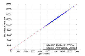
(a) Free Riders = 10 %, $\alpha=0.9$

(b) Free Riders = 10 %, $\alpha=0.6$

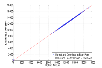
(c) Free Riders = 10 %, $\alpha=0.3$

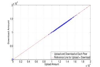
(d) Free Riders = 30 %, $\alpha=0.9$

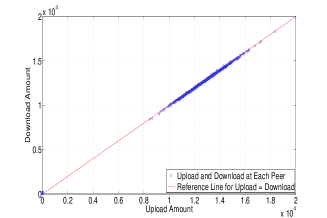
(e) Free Riders = 30 %, $\alpha=0.6$

(f) Free Riders = 30 %, $\alpha=0.3$

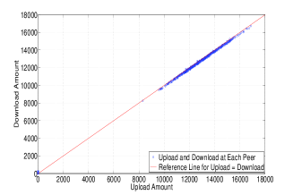
(g) Free Riders = 50 %, $\alpha=0.9$

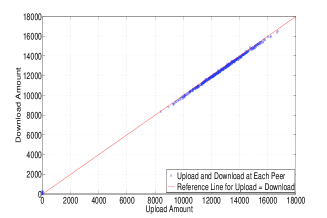
(h) Free Riders = 50 %, $\alpha=0.6$

(i) Free Riders = 50 %, $\alpha=0.3$

(j) Free Riders = 70 %, $\alpha=0.9$

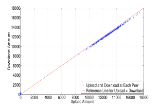
(k) Free Riders = 70 %, $\alpha=0.6$

(l) Free Riders = 70 %, $\alpha=0.3$

Fig. 2: Upload and Download Amount at Each Peer for SBCI in Simple Model for Simple Procedure of Peer Selection. Free-riders are varied from $10\%-70\%$ and the value of $\alpha$ is taken as $0.9,0.6$ and 0.3

TABLE I: AAD and $\%$ of Rejections for SBCI in Simple Model for Simple Procedure of Peer Selection

S.N.	$\alpha$	Free-riders	AAD	$\%$ of Rejections
$1$	0.9	10%	0.103772	1.817
$2$	0.9	30%	0.303675	0.127
$3$	0.9	50%	0.505119	0.023
$4$	0.9	70%	0.707233	0.008
$5$	0.6	10%	0.103667	0.064
$6$	0.6	30%	0.303652	0.009
$7$	0.6	50%	0.505459	0.006
$8$	0.6	70%	0.707117	0.003
$9$	0.3	10%	0.103844	0.009
$10$	0.3	30%	0.303671	0.002
$11$	0.3	50%	0.505088	0.001
$12$	0.3	70%	0.707069	0

We conducted the simulation experiment for simple procedure of peer selection, as explained in Section 5. Bandwidth of all the peers is assumed to be same. For simple model, simulation results for SBCI are shown in Fig. 2. Corresponding $AAD$ and percentage of rejections among cooperative peers are shown in Table I. We can observe from this figure that in initial transactions, free-riders got some resources after that their SBCI become zero, which disqualify them in taking any resources from the network. For all other peers, upload to download ratio is very close to the reference line, thus algorithm is able to maintain the fairness in the network. We can observe from Table I that the percentage of rejections among the cooperative peers are more for higher values of $\alpha$. Because for higher values of $\alpha$, threshold value of SBCI will be higher. But its impact on $AAD$ is not very significant in this model.

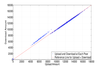
(a) Free Riders = 20 %, $\alpha=0.9$

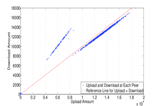
(b) Free Riders = 20 %, $\alpha=0.6$

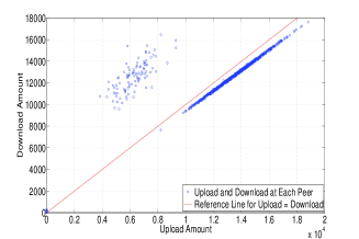
(c) Free Riders = 20 %, $\alpha=0.3$

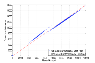
(d) Free Riders = 40 %, $\alpha=0.9$

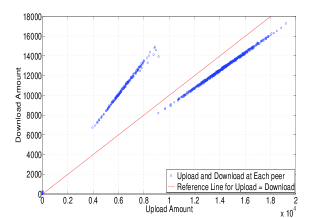
(e) Free Riders = 40 %, $\alpha=0.6$

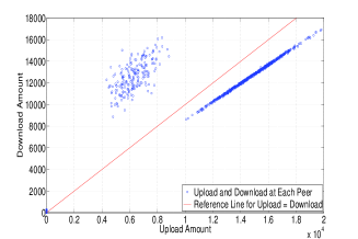
(f) Free Riders = 40 %, $\alpha=0.3$

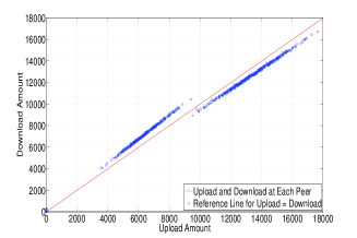
(g) Free Riders = 60 %, $\alpha=0.9$

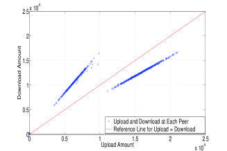
(h) Free Riders = 60 %, $\alpha=0.6$

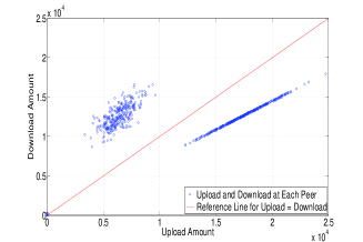
(i) Free Riders = 60 %, $\alpha=0.3$

Fig. 3: Upload and Download Amount at Each Peer for SBCI in Adaptive Model for Simple Procedure of Peer Selection. Free-riders are varied from $20\%-60\%$ and the value of $\alpha$ is taken as $0.9,0.6$ and 0.3

TABLE II: AAD and $\%$ of Rejections for SBCI in Adaptive Model for Simple Procedure of Peer Selection

S.N.	$\alpha$	Free-riders	AAD	$\%$ of Rejections
$1$	0.9	20%	0.118469	1.87
$2$	0.9	40%	0.236766	0.606
$3$	0.9	60%	0.354868	0.198
$4$	0.6	20%	0.175055	0.054
$5$	0.6	40%	0.351099	0.028
$6$	0.6	60%	0.527092	0.011
$7$	0.3	20%	0.200618	0.020
$8$	0.3	40%	0.401786	0.011
$9$	0.3	60%	0.600657	0.008

In Adaptive Model, free-riders earn the SBCI and thereafter use this SBCI to download maximum resources from the network. Simulation results for this model are shown in Fig. 3. Corresponding $AAD$ and percentage of rejections among cooperative peers are shown in Table II. We can observe from this figure that for higher $\alpha$, algorithm performs better. For $\alpha=0.9$, even in the presence of a large number of free-riders, the algorithm is able to balance the upload and download amount in the network. We can also observe from Table II that for higher $\alpha$ the percentage of rejection among cooperative peers is higher but corresponding $AAD$ is very less. Thus, impact of $\alpha$ is clearly evident.

And finally, we conducted the simulation for SBCI in Extreme Model. Results for upload and download at each peer are shown in Fig. 4. Corresponding $AAD$ and percentage of rejections among cooperative peers are shown in Table III. We can observe from the figure that for $\alpha=0.9$ the algorithm is able to balance the upload and download amount in the network. For $\alpha=0.9$, at the cost of less than 2% of rejections among the cooperative peers, algorithm is able to maintain $AAD$ as 0.211228.

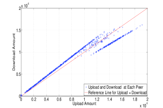
(a) Free Riders = 80%, $\alpha=0.9$

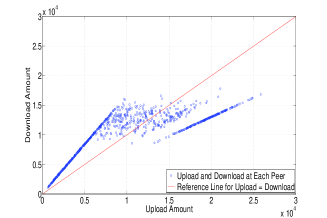
(b) Free Riders = 80%, $\alpha=0.6$

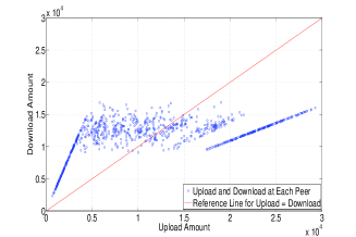
(c) Free Riders = 80%, $\alpha=0.3$

Fig. 4: Upload and Download Amount at Each Peer for SBCI in Extream Model for Simple Procedure of Peer Selection. At the beginning of simulation, 10% peers are free-riders. After completion of every 12.5% of total transactions, 10% more peers convert themselves to free-riders. The value of $\alpha$ is taken as $0.9,0.6$ and 0.3

TABLE III: AAD and $\%$ of Rejections for SBCI in Simple Model for Simple Procedure of Peer Selection

S.N.	$\alpha$	Free-riders	AAD	$\%$ of Rejections
$1$	0.9	80%	0.211228	1.794
$2$	0.6	80%	0.423116	0.068
$3$	0.3	80%	0.567303	0.010

We also reported the simulation results of GC for all peer distribution models in Fig. 5. Corresponding $AAD$ and percentage of rejections among cooperative peers are reported in Table IV. We can see from the figure that GC can also balance the upload and download amounts in each peer. In Adaptive Model and in Extreme Model GC can maintain better fairness compared to SBCI but the percentage of rejections among cooperative peers are higher in GC for all the models. Thus, it is less efficient compared to SBCI.

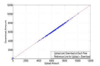
(a) Simple Model, Free Riders = 30%

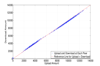
(b) Adaptive Model, Free Riders = 60%

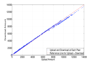
(c) Extreme Model, Free Riders = 80%

Fig. 5: Upload and Download Amount at Each Peer for best case of GC, i.e., $\alpha=0.8,\beta=0.2$ in different distribution models for Simple Procedure of Peer Selection.

TABLE IV: AAD and $\%$ of Rejections for Different Distribution Model in Best case of GC for Simple Procedure of Peer Selection

S.N.	Model	Free-riders	AAD	$\%$ of Rejections
$1$	Simple	30%	0.3059	33.657
$2$	Adaptive	60%	0.3146	16.27
$3$	Extreme	80%	0.1370	19.269

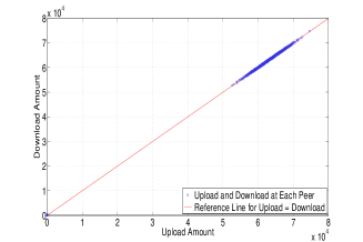
(a) Free Riders = 10%, $\alpha=0.9$

(b) Free Riders = 10%, $\alpha=0.6$

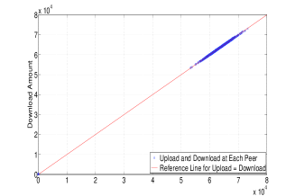
(c) Free Riders = 10%, $\alpha=0.3$

(d) Free Riders = 30%, $\alpha=0.9$

(e) Free Riders = 30%, $\alpha=0.6$

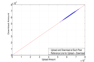
(f) Free Riders = 30%, $\alpha=0.3$

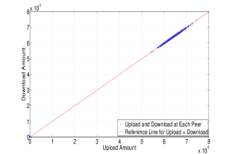
(g) Free Riders = 50%, $\alpha=0.9$

(h) Free Riders = 50%, $\alpha=0.6$

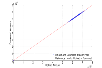
(i) Free Riders = 50%, $\alpha=0.3$

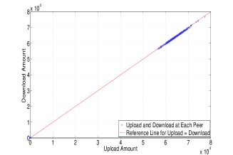
(j) Free Riders = 70%, $\alpha=0.9$

(k) Free Riders = 70%, $\alpha=0.6$

(l) Free Riders = 70%, $\alpha=0.3$

Fig. 6: Upload and Download Amount at Each Peer in the Presence of $10\%-70\%$ Free-riders for Different values of $\alpha$. Peer selection approach is based on the problem of ”College Admission and The Stability of Marriage”. Bandwidth distribution is as type 1.

TABLE V: AAD and $\%$ of Rejections for SBCI in Simple Model for Stable merriage approach with two different bandwith peers

S.N.	$\alpha$	Free-riders	AAD	$\%$ of Rejections
$1$	0.9	10%	0.102265	1.0114
$2$	0.9	30%	0.301927	0.287
$3$	0.9	50%	0.501482	0.0244
$4$	0.9	70%	0.701471	0.0026
$5$	0.6	10%	0.102312	0.046
$6$	0.6	30%	0.30196	0.0134
$7$	0.6	50%	0.50149	0.0034
$8$	0.6	70%	0.701432	0.0008
$9$	0.3	10%	0.102367	0.0114
$10$	0.3	30%	0.301967	0.0036
$11$	0.3	50%	0.501484	0.0016
$12$	0.3	70%	0.701441	0

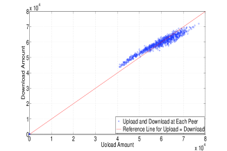
(a) Free Riders = 10%, $\alpha=0.9$

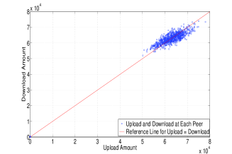
(b) Free Riders = 10%, $\alpha=0.6$

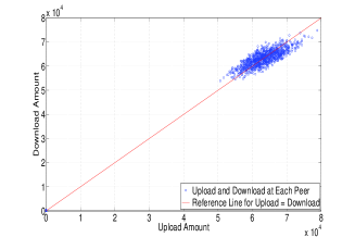
(c) Free Riders = 10%, $\alpha=0.3$

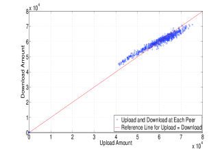
(d) Free Riders = 30%, $\alpha=0.9$

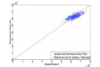
(e) Free Riders = 30%, $\alpha=0.6$

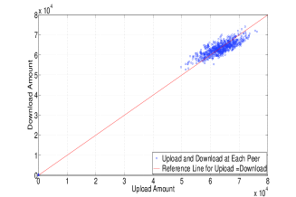
(f) Free Riders = 30%, $\alpha=0.3$

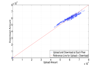
(g) Free Riders = 50%, $\alpha=0.9$

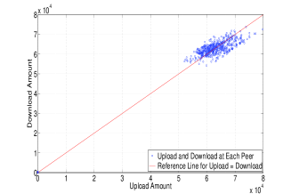
(h) Free Riders = 50%, $\alpha=0.6$

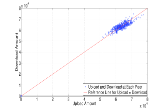
(i) Free Riders = 50%, $\alpha=0.3$

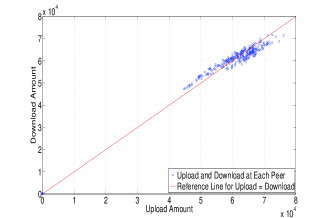
(j) Free Riders = 70%, $\alpha=0.9$

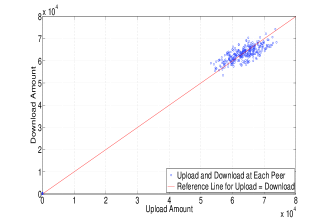
(k) Free Riders = 70%, $\alpha=0.6$

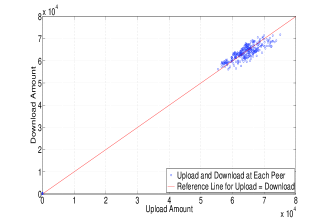
(l) Free Riders = 70%, $\alpha=0.3$

Fig. 7: Upload and Download Amount at Each Peer in the Presence of $10\%-70\%$ Free-riders for Different values of $\alpha$. Peer selection approach is based on the problem of ”College Admission and The Stability of Marriage”. Bandwidth distribution is as type 2.

TABLE VI: AAD and $\%$ of Rejections for SBCI in Simple Model for Stable merriage approach with ten different bandwith peers

S.N.	$\alpha$	Free-riders	AAD	$\%$ of Rejections
$1$	0.9	10%	0.131826	6.1534
$2$	0.9	30%	0.322511	4.2034
$3$	0.9	50%	0.515015	2.3352
$4$	0.9	70%	0.709604	0.9604
$5$	0.6	10%	0.128717	0.4344
$6$	0.6	30%	0.327149	0.2746
$7$	0.6	50%	0.520278	0.1396
$8$	0.6	70%	0.710663	0.0348
$9$	0.3	10%	0.130575	0.1214
$10$	0.3	30%	0.323463	0.0652
$11$	0.3	50%	0.514418	0.024
$12$	0.3	70%	0.70845	0.0054

6.4 Simulation Results of College Admission and The Stability of Marriage Based Approach For the Peer Selection

We also conducted the experiment for college admission and the stability of marriage based approach for the peer selection. For simplicity, we considered only Simple model. Bandwidth of peers is assumed to be different, so that they can also include the bandwidth, as a criteria for peer selection. Selection of peer for downloading and uploading is done according to Algorithm 3. The stable match for uploader and downloader is made downloader optimal. To observe the impact of heterogeneity, we simulated the Simple Model for two different types of bandwidth distributions, i.e., type 1 and type 2.

In type 1, half of the peers have bandwidth 10 units and the rest have 20 units. Simulation results for this type are shown in Fig. 6. Corresponding $AAD$ and percentage of rejections among cooperative peers are shown in Table V. We can see from the figure that upload and download amount increases in each peer compared to simple procedure. Because each peer, who request for resources, is getting some option for downloading. Uploads and downloads in each peer are close to the reference line and corresponding $AAD$ are lesser compared to simple procedure. Thus, the algorithm is able to balance the upload and download amount in each peer.

In type 2, 10% of the peers have bandwidth 10 units, next 10% of the peers have bandwidth 20 units, next 10% of peers have bandwidth 30 units and so on. In this way, last 10% of peers will have bandwidth 100 units. Simulation results for this type are shown in Fig. 7. Corresponding $AAD$ and percentage of rejections among cooperative peers are shown in Table VI. We can observe from this figure that upload and download amounts for most of the peers are far from reference line and corresponding $AAD$ are also higher. Thus, the impact of heterogeneity is clearly evident. It also supports the argument that if we will select the source peer according to bandwidth rather than SBCI, we will loose the fairness in the network.

7 Conclusion

In this work, we proposed a new algorithm to make the P2P network fair and efficient. The algorithm ranks the peers based on their simplified biased contribution index (SBCI) which can vary from 0 to 1. Estimation of SBCI is based on two factors, the resources contributed by the peer and the SBCI of peer with whom it is transacting. We propose the design rules to make the network fair and efficient. With the help of mathematical justification, we have shown that our algorithm can fulfill all the design objectives and is able to maintain the fairness in the network. This algorithm can be implemented in the truly distributed fashion. Since, no iterative calculation is needed, it can be implemented with lesser message overhead and storage capacity.

We proposed two different peer selection approaches, namely simple procedure and college admission and the stability of marriage based approach. Simulation results show that the algorithm is able to suppress the free-riders in highly free-riding environment. The algorithm is also able to suppress the dynamic free-riders, i.e., those who change their behavior dynamically.

In future, we would like to implement this mechanism in unstructured P2P network.

H e was born in Uttarkashi, India. He is currently pursuing Ph.D in the Department of Electrical Engineering at IIT, Kanpur. His research interests include Peer-to-Peer Networks, Wireless Sensor Networks, Complex Networks, Social Networks, Solution of non-linear equations, Application of Linear Algebra and Game theory in Networks.

H e was born in Delhi, India. He was awarded Ph.D for his work on optical amplifier placement problem in all-optical broadcast networks in 1997 by IIT Delhi. In July 1997, he joined EE Department, IIT Kanpur. He was given AICTE young teacher award in 2003. Currently, he is working as professor. He is fellow of IETE, senior member of IEEE and ICEIT, and member ISOC. He has interests in telecommunications’ networks specially optical networks, switching systems, mobile communications, distributed software system design. He has supervised 10 Ph.D and more than 125 M.Tech theses so far. He has filed three patents for switch architectures, and have published many journal and conference research publications. He has also written lecture notes on Digital Switching which are distributed as open access content through content repository of IIT Kanpur. He has also been involved in opensource software development. He has started Brihaspati (brihaspati.sourceforge.net) initiative, an opesource learning management system, BrihaspatiSync – a live lecture delivery system over Internet, BGAS – general accounting systems for academic institutes.

References

- [1] J. S. Otto, M.A. Sanchez, D. R. Choffnes, F.E. Bustamante, and G. Siganos, “On Blind Mice and the Elephant - Understanding the Network Impact of a Large Distributed System,” Proc. of ACM SIGCOMM, conference 2011. pp. 110- 121, 2011.
- [2] Sandvine, Waterloo, Canada, “Sandvine June 2016 global Internet phenomena report,” 2016 [Online]. Available: https://www.sandvine.com/trends/global-internet-phenomena/
- [3] M. Karakaya, I. Korpeoglu, and O. Ulusoy, “Free riding in peer-topeer networks,” IEEE Internet Comput., vol. 13, no. 2, pp. 92–98, March-April 2009.
- [4] H. Nishida and T. Nguyen,”A Global Contribution Approach to Maintain Fairness in P2P networks” IEEE Tran. on Parallel and Distributed system, vol.21, no.6, June 2010.
- [5] S. K. Awasthi and Y. N. Singh,”Biased Contribution Index: A Simpler Mechanism to Maintain Fairness in Peer to Peer Networks”https://arxiv.org/pdf/1606.00717.pdf, June 2016.
- [6] M. Feldman, K. Lai, I. Stoica, and J. Chuang, “Robust Incentive Techniques for Peer-to-Peer Networks,” Proc. Fifth ACM Conf. Electronic Commerce, pp. 102-111, May 2004.
- [7] P. Garbacki, D. H. J. Epema and M. Steen, ”An Amortized Tit-For-Tat Protocol for Exchanging Bandwidth Instead of Content in P2P Networks,” First Int’l Conf. Self-Adaptive and Self-Organizing Systems, pp. 119-228, 2007.
- [8] Q. Lian, Y. Peng, M. Yang, Z. Zhang, Y. Dai, and X. Li, “Robust Incentives via Multi-Level Tit-for-Tat,” Concurrency and Computation: Practice & Experience, vol. 20, pp. 167-178, 2008.
- [9] J. J. D. Mol, J. A. Pouwelse, D. H. J. Epema, and H. J. Sips, “Give-to-Get: Free-Riding Resilient Video-on-Demand in P2P Systems,”Proc. Multimedia Computing and Networking, pp. 681804-1-681804-8,2008.
- [10] V. S. Borkar, R. Makhijani and R. Sundaresan, ”Asynchronous Gossip for Averaging and Spectral Ranking,” IEEE Journal Of Selected Topics in Signal Processing, vol. 8, no. 4, pp. 703-716, August 2016.
- [11] S. Saroiu, P. K. Gummadi, and S. D. Gribble. ”A Measurement Study of Peer-to-Peer File Sharing Systems.”In Proceedings of Multimedia Computing and Networking 2002 (MMCN ’02), San Jose, CA, USA, January 2002.
- [12] M. Feldman, C. Papadimitriou, J. Chuang, and I. Stoica, ”Free-Riding and Whitewashing in Peer-to-Peer Systems,” Proc. ACM SIGCOMM Workshop Practice and Theory of Incentives in Networked Systems (PINS), pp. 228-236, August 2004.
- [13] K. Eger and U. Killat, ”Fair Resource Allocation in Peer-to-Peer Networks (Extended Version),”Computer Comm., vol. 30, no. 16, pp. 3046-3054, November 2007.
- [14] H. Park and M. van der Schaar, ”A Framework for Foresighted Resource Reciprocation in P2P Networks,” IEEE Trans. Multimedia, vol. 11, no. 1, pp. 101-116, January 2009.
- [15] R. Izhak-Ratzin, H. Park and M. van der Schaar,”Online Learning in BitTorrent Systems,” IEEE Tran. on Parallel and Distributed system, vol. 23, no. 12, pp. 2280-2288, December 2012.
- [16] A. Sherman, J. Nieh, and C. Stein,”FairTorrent: A Deficit-Based Distributed Algorithm to Ensure Fairness in Peer-to-Peer Systems” IEEE/ACM Trans. Networking, vol. 20, no. 5, pp.1361-1374, October 2012.
- [17] J. Park and M. van der Schaar,”A Game Theoretic Analysis of Incentives in Content Production and Sharing Over Peer-to-Peer Networks,” IEEE Journal of Selected Topics in Signal Processing, vol. 4, no. 4, August 2010.
- [18] Y. Chen, B. Wang, W. Sabrina Lin,Y. Wu, and K. J. Ray Liu,”Cooperative Peer-to-Peer Streaming: An Evolutionary Game-Theoretic Approach,” IEEE Trans. on Circuit and Systems for Video Technology, vol. 20, no. 10 , pp. 1346-1357, October 2010.
- [19] R. T. B. Ma, S. C. M. Lee, J. C. S. Lui and D. K. Y. Yau, ”Incentive and Service Differentiation in P2P Networks: A Game Theoretic Approach,”IEEE/ACM Trans. Networking, vol. 14, no. 5, pp. 978-991, October 2006.
- [20] B. Cohen, ”Incentives build robustness in BitTorrent,” presented at the 1st Workshop Econ. Peer-to-Peer Syst., Jun. 2003.
- [21] D. Levin, K. LaCurts, N. Spring, and B. Bhattacharjee, “BitTorrent is an auction: Analyzing and improving BitTorrent’s incentives,” in Proceedings of the ACM SIGCOMM, pp. 243–254, August 2008.
- [22] F. Wu and L. Zhang. Proportional response dynamics leads to market equilibrium. In ACM STOC, 2007.
- [23] S. K. Awasthi and Y. N. Singh, ”Absolute Trust:Algorithm for Aggregation of Trust in Peer to Peer Network”, http://arxiv.org/abs/1601.01419
- [24] S. D. Kamvar, M. T. Schlosser and H. Garcia-Molina, ”The eigentrust algorithm for reputation management in P2P networks,” Proc. of the 12th international conference on World Wide Web, ser. WWW ’03. New York, USA: ACM, pp. 640–651, 2003.
- [25] S. K. Awasthi and Y. N. Singh, ”Generalized Analysis of Convergence of Absolute Trust in Peer to Peer Networks,” IEEE Communication Letters, vol. 20, no. 7, July 2016.
- [26] Ahmet Burak Can and Bharat Bhargava, ”SORT: A Self-ORganizing Trust Model for Peer-to-Peer Systems,” IEEE Trans. On Dependable and Secure Computing, vol. 10, no. 1, pp. 14-27, January/February 2013.
- [27] I. Stoica, R. Morris, D. Nowell, D. Karger, M. Kaashoek, F. Dabek and H. Balakrishnan, ”Chord: A Scalable Peer-to-Peer Lookup Protocol for Internet Applications,” ACM SIGCOMM Computer Comm. Rev., vol. 31, no. 4, pp. 149-160, 2001.
- [28] S. Ratnasamy, P. Francis, M. Handley, R. Karp and S. Shenker, ”A scalable content-addressable network,” Proc. of ACM SIGCOMM ’01 conference on Applications, technologies, architectures, and protocols for computer communications, pp. 161-172, August 2001.
- [29] A. Rowstron and P. Druschel, ”Pastry: Scalable, distributed object location and routing for large-scale peer-to-peer systems,” Proc. of the Middleware’01 IFIP/ACM International Conference on Distributed Systems Platforms Heidelberg, pp. 329-350, 2001.
- [30] B. Y. Zhao, L. Huang, J. Stribling, S. C. Rhea, A. D. Joseph and J. D. Kubiatowicz, ”Tapestry: A resilient global-scale overlay for service deployment,” IEEE Journal on Selected Areas in Communications, vol. 22, no. 1, pp.41–53, January 2004.
- [31] D. Gale and L. S. Shapley, ”College admissions and the stability of marriage,” The American Mathematical Monthly, vol. 69, no. 1, pp.9-15, January 1962.
- [32] Xiaoyong Li, Feng Zhou and Xudong Yang, ”Scalable Feedback Aggregating (SFA) Overlay for Large-Scale P2P Trust Management,” IEEE Trans. Parallel and Distributed Systems, vol. 23, No. 10, pp.1944-1957, October 2012.
- [33] Z. Liang and W. Shi, ”Analysis of ratings on trust inference in open environments,” Performance Evaluation, vol. 65, no. 2, pp. 99-128, 2008.
- [34] Uri Wilensky, https://ccl.northwestern.edu/netlogo/, 2015.
- [35] Matei Ripeanu, Adriana Iamnitchi, and Ian Foster, ”Mapping the Gnutella Network: Properties of Large-Scale Peer-to-Peer Systems and Implications for System Design,” IEEE Internet Computing Journal special issue on peer-to-peer networking, vol. 6(1), 50-57, January/February 2002.
- [36] R. Cuevas, M. Kryczka, A. Cuevas, S. Kaune, C. Guerrero, and R. Rejaie. ”Unveiling the Incentives for Content Publishing in Popular BitTorrent Portals,” IEEE/ACM Trans. Networking, vol. 21, no. 5, pp.1421-1435, October 2013.
- [37] Denis Serre, Matrices Theory and Applications, Springer-Verlag New York, Inc., 2002.