Coarse Grained Exponential Variational Autoencoders

Abstract

Variational autoencoders (VAE) often use Gaussian or category distribution to model the inference process. This puts a limit on variational learning because this simplified assumption does not match the true posterior distribution, which is usually much more sophisticated. To break this limitation and apply arbitrary parametric distribution during inference, this paper derives a semi-continuous latent representation, which approximates a continuous density up to a prescribed precision, and is much easier to analyze than its continuous counterpart because it is fundamentally discrete. We showcase the proposition by applying polynomial exponential family distributions as the posterior, which are universal probability density function generators. Our experimental results show consistent improvements over commonly used VAE models.

1 Introduction

Variational autoencoders Kingma & Welling (2014) and its variants Rezende et al. (2014); Sohn et al. (2015); Salimans et al. (2015); Burda et al. (2016); Serban et al. (2016) combine the two powers of variational Bayesian learning Jordan et al. (1999) with strong generalization and a standard learning objective, and deep learning with flexible and scalable representations. They are attracting decent attentions, producing state-of-the-art performance in semi-supervised learning Kingma et al. (2014) and image generation Gregor et al. (2015), and are getting applied in diverse areas such as deep generative modeling Rezende et al. (2014), image segmentation Sohn et al. (2015), clustering Dilokthanakul et al. (2017), and future prediction from images Walker et al. (2016).

This paper discusses unsupervised learning with VAE which pipes an inference model $q(\bm{z}\,|\,\bm{x})$ with a generative model $p(\bm{x}\,|\,\bm{z})$, where $\bm{x}$ and $\bm{z}$ are observed and latent variables, respectively. A simple parameter-free prior $p(\bm{z})$ combined with $p(\bm{x}\,|\,\bm{z})$ parameterized by a deep neural network results in arbitrarily flexible representations. However, its (very complex) posterior $p(\bm{z}\,|\,\bm{x})$ must be within the representation power of the inference machine $q(\bm{z}\,|\,\bm{x})$, so that the variational bound is tight and variational learning is effective.

In the original VAE Kingma & Welling (2014), $q(\bm{z}\,|\,\bm{x})$ obeys a Gaussian distribution with a diagonal covariance matrix. This is a very simplified assumption, because Gaussian is the maximum entropy (least informative) distribution with respect to prescribed mean and variance and has one single mode, while human inference can be ambiguous and can have a bounded support when we exclude very unlikely cases de Haan & Ferreira (2006).

Many recent works try to tackle this limitation. Jang et al. (2017) extended VAE to effectively use a discrete latent $\bm{z}$ following a category distribution (e.g. Bernoulli distribution). Kingma et al. (2014) extended the latent structure with a combination of continuous and discrete latent variables (class labels) and applied the model into semi-supervised learning. Similarly, Shu et al. (2016) and Dilokthanakul et al. (2017) proposed to use a Gaussian mixture latent model in VAE. Serban et al. (2016) applied a piecewise constant distribution on $\bm{z}$.

This work contributes a new ingredient in VAE model construction. To tackle the difficulty in dealing with complex probability density function (pdf) $p(\bm{z})$ $(\bm{z}\in\mathcal{Z})$, we generate instead a semi-continuous $\bm{z}\in\mathcal{Z}$, by first discretizing the support $\mathcal{Z}$ into a grid, then drawing a discrete sample $\bm{y}$ based on the corresponding probability mass function (pmf), and then reconstruct $\bm{y}$ into $\bm{z}\in\mathcal{Z}$. This coarse grain (CG) technique can help apply any pdf into VAE. Hence we apply a bounded polynomial exponential family (BPEF) as the underlying $p(\bm{z})$, which is a universal pdf generator. This fits in the spirit of neural networks because the prior and posterior are not hand-crafted but learned by themselves.

This contribution blends theoretical insights with empirical developments. We present CG, BPEF, information monotonicity, etc., that are useful ingredients for general VAE modeling. Notably, we present a novel application scenario with new analysis on the Gumbel softmax trick Jang et al. (2017); Maddison et al. (2016). We assemble these components into a machine CG-BPEF-VAE and present empirical results on unsupervised density estimation, showing improvements over vanilla VAE Kingma & Welling (2014) and category VAE Jang et al. (2017). We present a novel perspective with theoretical analysis of VAE learning, with guaranteed bounds derived from information geometry Amari (2016).

This paper is organized as follows. Sec. 2 reviews the basics of VAE. Sec. 3 introduces CG-VAE and its implementation CG-BPEF-VAE. Sec. 4 performs an empirical study on two different datasets. Sec. 5 gives a theoretical analysis on VAE learning. Sec. 6 states our concluding remarks.

2 Prerequisites: Variational Autoencoders

This section covers the basics from a brief introduction of variational Bayes to previous works on VAE. A generative model can be specified by a joint distribution between the observables $\bm{x}$ and the hidden variables $\bm{z}$, that is, $p(\bm{x},\bm{z}\,|\,\bm{\theta})=p(\bm{z}\,|\,\bm{\theta}_{z})p(\bm{x}\,|\,\bm{z},\bm{\theta}_{x|z})$ where $\bm{\theta}=(\bm{\theta}_{z},\bm{\theta}_{x|z})$. By Jensen’s inequality,

$$-\log p(\bm{x}\,|\,\bm{\theta})=-\log\int q(\bm{z}\,|\,\bm{x},\bm{\varphi})\frac{p(\bm{x},\bm{z}\,|\,\bm{\theta})}{q(\bm{z}\,|\,\bm{x},\bm{\varphi})}d\bm{z}$$

$$\leq\int q(\bm{z}\,|\,\bm{x},\bm{\varphi})\log\frac{q(\bm{z}\,|\,\bm{x},\bm{\varphi})}{p(\bm{x},\bm{z}\,|\,\bm{\theta})}d\bm{z}\left(\stackrel{{\scriptstyle def}}{{=}}\mathcal{L}(\bm{\theta},\bm{\varphi})\right),$$ (1)

for any $q(\bm{z}\,|\,\bm{x},\bm{\varphi})$. The upper bound $\mathcal{L}(\bm{\theta},\bm{\varphi})$ on the RHS is known as the “variational free energy”. We have

$$\mathcal{L}(\bm{\theta},\bm{\varphi})=\underbrace{\mathrm{KL}(q(\bm{z}\,|\,\bm{x},\bm{\varphi}):p(\bm{z}\,|\,\bm{\theta}_{z}))}_{term_{1}}$$

$$\hskip 50.00008pt\underbrace{-\int q(\bm{z}\,|\,\bm{x},\bm{\varphi})\log{p}(\bm{x}\,|\,\bm{z},\bm{\theta}_{x|z})d\bm{z}}_{term_{2}},$$

where $\mathrm{KL}(\cdot:\cdot)$ denotes the Kullback-Leibler (KL) divergence. (We will use $term_{1}$ and $term_{2}$ as short-hands for the two terms whose sum is $\mathcal{L}(\bm{\theta},\bm{\varphi})$. One has to remember that they are functions of $\bm{\theta}$ and $\bm{\varphi}$.) We therefore minimize the free energy with respect to both $\bm{\theta}$ and $\bm{\varphi}$ so as to minimize $-\log{p}(\bm{x}\,|\,\bm{\theta})$. The gap of the bound in Sec. 2 is $\mathcal{L}(\bm{\theta},\bm{\varphi})-(-\log p(\bm{x}\,|\,\bm{\theta}))=\mathrm{KL}\left(q(\bm{z}\,|\,\bm{x},\bm{\varphi}):p(\bm{z}\,|\,\bm{x},\bm{\theta})\right)$, which can be small as long as the parameter manifold of $q(\bm{z}\,|\,\bm{x},\bm{\varphi})$ (e.g. constructed based on the mean field technique, Jordan et al. 1999) encompasses a good estimation of the true posterior.

VAE Kingma & Welling (2014) assume the following generative process. The prior $p(\bm{z}\,|\,\bm{\theta}_{z})=G(\bm{z}\,|\,\bm{0},\bm{I})$ is parameter free, where $G(\cdot\,|\,\bm{\mu},\bm{\Sigma})$ denotes a Gaussian distribution with mean $\bm{\mu}$ and covariance matrix $\bm{\Sigma}$. Denote $\dim\bm{x}=D$ and $\dim\bm{z}=d$. The conditional mapping $p(\bm{x}\,|\,\bm{z},\bm{\theta})=\prod_{i=1}^{D}p\left(x_{i}\,|\,f(\bm{z},\bm{\theta})\right)$ is parametrized by a neural network $f(\bm{z},\bm{\theta})$ with input $\bm{z}$ and parameters $\bm{\theta}$. For binary $\bm{x}$, $p(x_{i}\,|\,\cdot)$ is a Bernoulli distribution; for continuous $\bm{x}$, $p(x_{i}\,|\,\cdot)$ can be univariate Gaussian. This gives a very flexible $p(\bm{x}\,|\,\bm{\theta})$ to adapt the complex data manifold.

In this case, it is hard to select the parameter form of $q(\bm{z}\,|\,\bm{x},\bm{\varphi})$, as the posterior $p(\bm{z}\,|\,\bm{x},\bm{\varphi})$ has no closed form solution. VAE borrows again the representation power of neural networks and lets $q(\bm{z}\,|\,\bm{x},\bm{\varphi})=G(\bm{z}\,|\,\bm{\mu}(\bm{x},\bm{\varphi}),\,\mathtt{diag}(\bm{\lambda}(\bm{x},\bm{\varphi})))$, where $\bm{\mu}(\bm{x},\bm{\varphi})$ and $\bm{\lambda}(\bm{x},\bm{\varphi})$ are both neural networks with input $\bm{x}$ and parameters $\bm{\varphi}$, and $\mathtt{diag}(\cdot)$ means a diagonal matrix constructed with a given diagonal vector. The assumption of a diagonal covariance is for reducing the network size so as to be efficient and to control overfitting.

Since the KL of Gaussians is available in closed form, $term_{1}$ has an analytical solution. In order to solve the integration in $term_{2}$, VAE employs a reparameterization trick. It draws $L$ i.i.d. samples $\bm{\epsilon}^{1},\cdots,\bm{\epsilon}^{L}\sim{}G(\bm{\epsilon}\,|\,\bm{0},\bm{I})$, where $\bm{I}$ is the identity matrix. Let $\bm{z}^{l}=\bm{\mu}(\bm{x},\bm{\varphi})+\bm{\lambda}(\bm{x},\bm{\varphi})\circ\bm{\epsilon}^{l}$, where “$\circ$” denotes element-wise product. Then $\bm{z}^{l}\sim{G}(\bm{z}\,|\,\bm{\mu}(\bm{x},\bm{\varphi}),\mathtt{diag}(\bm{\lambda}(\bm{x},\bm{\varphi})))$. Hence

$$term_{2}\approx-\frac{1}{L}\sum_{l=1}^{L}\log p\left(\bm{x}\,|\,\bm{\mu}(\bm{x},\bm{\varphi})+\bm{\lambda}(\bm{x},\bm{\varphi})\circ\bm{\epsilon}^{l},\bm{\theta}\right).$$

This trick allows error to backpropagate through the random mapping $(\bm{\mu},\bm{\lambda})\leadsto\bm{z}$.

Then $\mathcal{L}(\bm{\theta},\bm{\varphi})=term_{1}+term_{2}$ can be expressed as simple arithmetic operations of the outputs of the hidden layer and the last layer. It can therefore be optimized e.g. with stochastic gradient descent. The optimization technique is called stochastic gradient variational Bayes (SGVB). The resulting architecture is presented in fig. 1(a).

(a) Gaussian VAE

(b) Category VAE

(c) CG-BPEF-VAE

Figure 1: Architecture of three different VAEs. Blue indicates that the corresponding variable is continuous; red means discrete. CG-BPEF-VAE features a sandwich structure.

3 CG-BPEF-VAE

We would like to extend VAE to incorporate a general inference process, where the model can learn by itself a proper $p(\bm{z}\,|\,\bm{x},\bm{\varphi})$ within a flexible family of distributions, which is not limited to Gaussian or category distributions and can capture higher order moments of the posterior. We will therefore derive in this section a variation of VAE called CG-BPEF-VAE for Coarse-Grained Bounded Polynomial Exponential Family VAE.

3.1 Bounded Polynomial Exponential Family

We try to model the latent $\bm{z}$ with a factorable polynomial exponential family (PEF) (Cobb et al., 1983; Nielsen & Nock, 2016) probability density function:

$$p(\bm{z})=\prod_{j=1}^{d}\exp\left(\sum_{m=1}^{M}c_{jm}z_{j}^{m}-\psi(\bm{c}_{j})\right),$$ (2)

where $M$ is the polynomial order, $\bm{C}=(c_{jm})_{d\times{M}}$ denotes the polynomial coefficients, and $\psi$ is a convex cumulant generating function Amari (2016). This PEF family can be regarded as the most general parameterization, because with large enough $M$ it can approximate arbitrary finely any given $p(\bm{z})$ satisfying weak regularity conditions (Cobb et al., 1983).

Furthermore, we constrain $\bm{z}$ to have a bounded support so that $\bm{z}\in[-1,1]^{d}$, a hypercube. This gives $\bm{z}$ a focused density that is not wasted on unlikely cases, which is in contrast to Gaussian distribution with non-zero probability on the whole real line. This also allows one to easily explore extreme cases by setting $z_{j}$ to $\pm 1$ or beyond.

For example, if $M=2$, then the resulting $p(z_{j})\propto\exp\left(c_{j1}z_{j}+c_{j2}z_{j}^{2}\right)$ includes the truncated Gaussian distribution (with one mode) as a special case when $c_{j2}<0$. Moreover, the setting $c_{j2}\geq 0$ encompasses more general cases and can have at most two modes.

The two important elements in constructing a VAE model are ➀ the KL divergence between $q(\bm{z}\,|\,\bm{x},\bm{\varphi})$ and $p(\bm{z}\,|\,\bm{\theta}_{z})$ must have a closed form; ➁ a random sample of $q(\bm{z}\,|\,\bm{x},\bm{\varphi})$ can be expressed as a simple function between its parameters and some parameter-free random variables. Neither of these conditions are met for BPEF. We will address these difficulties in the remainder of this section.

3.2 Coarse Grain

Our basic idea is to reduce the BPEF pdf into a discrete distribution, then draw samples based on the pmf, then reconstruct the continuous sample.

We sample $R$ points uniformly on the interval $[-1,1]$:

$$\bm{\zeta}=\left(-1,-1+\frac{2}{R-1},\cdots,1-\frac{2}{R-1},1\right)^{\intercal},$$

where the $r$’th discrete value is $\zeta_{r}=\frac{2r-(R+1)}{R-1}$. For example, choosing $R=21$ results in a precision of 0.1. In correspondence to these $R$ locations, we assume for the $j$’th latent dimension a random $\bm{y}_{j}$ in $\Delta^{R-1}$, the $(R-1)$-dimensional probability simplex, so that $\sum_{r=1}^{R}y_{jr}=1$, $\forall{r}$, $y_{jr}\geq 0$. This $y_{jr}$ means the likelihood for $z_{j}$ taking the value $\zeta_{r}$. Intuitively, if we constrain $\bm{y}_{j}$ to be one-hot (with probability mass only on vertices of $\Delta^{R-1}$), and let $P(y_{jr}=1)\propto\exp(\sum_{m=1}^{M}c_{jm}\zeta_{r}^{m})$, then the expectation $z_{j}=\sum_{r=1}^{R}y_{jr}\zeta_{r}\in[-1,1]$ will be distributed like the BPEF in eq. 2.

However, to apply the reparameterization trick, it is not known how to express a random one-hot sample $\bm{y}_{j}$ as a simple function of the activation probabilities. Nor does Dirichlet distribution as a commonly-used density on $\Delta^{R-1}$ can do the trick.

This reparameterization problem of category distribution is studied recently Jang et al. (2017); Maddison et al. (2016) following earlier developments Kuzmin & Warmuth (2005); Maddison et al. (2014) on applying extreme value distributions de Haan & Ferreira (2006) to machine learning. Based on these previous studies, we let $\bm{y}_{j}$ follow a Concrete distribution Maddison et al. (2016), which is a continuous relaxation of the category distribution, with the key advantage that Concrete samples can be easily drawn to be applied to VAE. Details are explained as follows.

The standard Gumbel distribution Gumbel (1954) is defined on the support $g\in\Re$ with the cumulative distribution function $P\left(g\leq{}x\right)=e^{-e^{-x}}$. Therefore Gumbel samples can be easily obtained by inversion sampling $g=-\log(-\log{U})$, where $U$ is uniform on $(0,1)$. Let $g_{jr}$ follows standard Gumbel distribution, then the random variable $\bm{y}_{j}\in\Delta^{R-1}$ defined by

$$y_{jr}=\frac{\exp\left((g_{jr}+\phi_{jr})/T\right)}{\sum_{r=1}^{R}\exp\left((g_{jr}+\phi_{jr})/T\right)}$$

is said to follow a Concrete distribution with location parameter $\bm{\phi}_{j}$ and temperature parameter $T$: $\bm{y}_{j}\sim{}\mathrm{Con}(\bm{\phi}_{j},T)$. This distribution has a closed-form probability density function (see Maddison et al. 2016) and has the following fundamental property

$$\forall{r},\quad P\left(\lim_{T\to 0^{+}}y_{jr}=1\right)=P\left(y_{jr}>y_{jo},\forall{o\neq{r}}\right)$$

$$={\exp(\phi_{jr})}/{\sum_{r=1}^{R}\exp(\phi_{jr})}\;\left(\stackrel{{\scriptstyle def}}{{=}}\alpha_{jr}\right).$$ (3)

Basically, at the limit $T\to 0^{+}$, the density will be pushed to the vertices of $\Delta^{R-1}$, and Concrete random vectors $\bm{y}_{j}$ tend to be onehot, with activation probability of the $r$’th bit defined by $\alpha_{jr}$. Hence it can be considered as a relaxation Maddison et al. (2016) of the category distribution. See fig. 2 for an intuitive view of the Concrete distribution. There are heavy volumes of densities around the vertices.

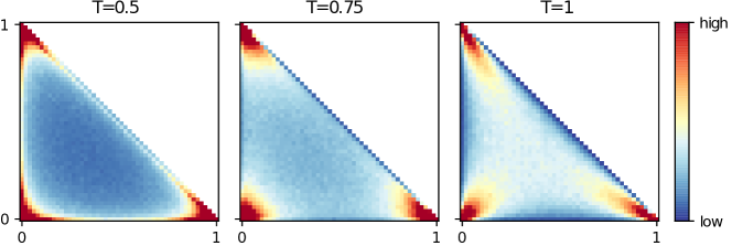
Figure 2: Density distribution of $\mathrm{Con}((1/3,1/3,1/3),T)$ over $\Delta^{2}$. The figure is generated by random sampling (see appendix for more figures and discussions).

In our case, let $\phi_{jr}=\sum_{m=1}^{M}c_{jm}\zeta_{r}^{m}$, then the odds for $y_{jr}$ activated (i.e., the probability for $z_{j}$ taking the value $\zeta_{r}$) will be proportional to $\exp\left(\sum_{m=1}^{M}c_{jm}\zeta_{r}^{m}\right)$ at the limit $T\to 0^{+}$. This provides a way to simulate the BPEF density.

3.3 The Model

Based on previous subsections, we assume the following generation process

$$\alpha_{jr}=\sum_{m=1}^{M}a_{jm}\zeta_{r}^{m},\quad{}p(\bm{y}\,|\,\bm{a})=\prod_{j=1}^{d}\mathrm{Con}\left(\bm{y}_{j}\,|\,\bm{\alpha}_{j},T\right),$$

$${z}_{j}(\bm{a})=\bm{y}_{j}^{\intercal}\bm{\zeta},\hskip 30.00005ptp(\bm{x}\,|\,\bm{z},\bm{\theta})=\prod_{i=1}^{D}p\left(x_{i}\,|\,f\left(\bm{z},\bm{\theta}\right)\right),$$

where $\bm{A}=(a_{jm})_{d\times{}M}$ is the parameters of the prior, and $f$ is defined by a neural network. One should always choose $M<R-1$, because the polynomial $\sum_{m=1}^{R-1}c_{jm}\zeta_{r}^{m}$ with $R-1$ free parameters can already represent any distribution in $\Delta^{R-1}$. The setting $M\geq{}R-1$ makes the polynomial structure redundant.

The corresponding inference process is given by

$$\beta_{jr} =\sum_{m=1}^{M}b_{jm}(\bm{x},\bm{\varphi})\zeta_{r}^{m},$$

$$q(\bm{y}\,|\,\bm{x},\bm{\varphi}) =\prod_{j=1}^{d}\mathrm{Con}\left(\bm{y}_{j}\,|\,\bm{\beta}_{j},T\right),$$

$$z_{j}(\bm{x},\bm{\varphi}) =\bm{y}_{j}^{\intercal}\bm{\zeta},$$

where $\bm{B}(\bm{x},\bm{\varphi})=(b_{jm}(\bm{x},\bm{\varphi}))_{d\times{}M}$ is defined by a neural network. By Monte Carlo integration, it is straightforward that

$$term_{2}\approx\frac{1}{L}\sum_{l=1}^{L}\sum_{i=1}^{D}\log p\left(x_{i}\,|\,f\left(\sum_{r=1}^{R}y_{\bullet{}r}^{l}\zeta_{r},\bm{\theta}\right)\right),$$

$$y_{jr}^{l}=\frac{\exp\left((g_{jr}^{l}+\sum_{m=1}^{M}b_{jm}(\bm{x},\bm{\varphi})\zeta_{r}^{m})/T\right)}{\sum_{r=1}^{R}\exp\left((g_{jr}^{l}+\sum_{m=1}^{M}b_{jm}(\bm{x},\bm{\varphi})\zeta_{r}^{m})/T\right)},$$

where $(g_{jr}^{l})$ is a 3D tensor of independent Gumbel variables, and the approximation becomes accurate when $L\to\infty$.

For simplicity, we assume $T$ to be the same scalar during generation and inference. We adopt a simple annealing process of $T$, starting from $T_{\max}$, exponentially decaying to $T_{\min}$ in the first half of training epochs, then keeping $T_{\min}$. The study Jang et al. (2017) implies that $T_{\min}=0.5\sim 1$ could be small enough to make the Concrete distribution approximate well a category distribution. The setting of $T_{\min}$ will affect the computation of $term_{1}$, which will be explained in the following subsection.

3.4 Information Mononicity

We need to compute $term_{1}$ which is the KL divergence between the posterior $p(\bm{z}\,|\,\bm{x},\bm{\varphi})$ the prior $p(\bm{z}\,|\,\bm{a})$. This is the most complex part because these pdfs are not in closed form. However, we know that as $T\to 0^{+}$ they converge to categories distributions over $R$ evenly spanned positions on $[-1,1]$ (the vector $\bm{\zeta}$). Therefore we approximate $term_{1}$ with the KL divergence between the corresponding category distributions, that is,

$$term_{1}\approx \sum_{j=1}^{d}\sum_{r=1}^{R}\Bigg{[}\frac{\exp(\beta_{jr})}{\sum_{r=1}^{R}\exp(\beta_{jr})}$$

$$\times\log\frac{\exp(\beta_{jr})/(\sum_{r=1}^{R}\exp(\beta_{jr}))}{\exp(\alpha_{jr})/(\sum_{r=1}^{R}\exp(\alpha_{jr}))}\Bigg{]}$$

$$= \sum_{j=1}^{d}\bigg{[}\frac{\sum_{r=1}^{R}\exp(\beta_{jr})(\beta_{jr}-\alpha_{jr})}{\sum_{r=1}^{R}\exp(\beta_{jr})}$$

$$+\log\sum_{r=1}^{R}\exp(\alpha_{jr})-\log\sum_{r=1}^{R}\exp(\beta_{jr})\bigg{]}.$$ (4)

In the rest of this subsection we give theoretical and empirical justifications of this approximation. KL divergence belongs to Csiszár’s $f$-divergence family and therefore satisfy the well-known information monotonicity Amari (2016). Basically, the support $V$ can be partitioned into subregions $\{V_{r}\}$ with zero volume overlap, so that $V=\uplus{}V_{r}$. Denote by $p_{1}(V_{r})=\int_{x\in{V}_{r}}p_{1}(x)\mathrm{d}x$ the probability mass of $V_{r}$, then $\sum_{r}p_{1}(V_{r})=1$ and the pmf $\{p_{1}(V_{r})\}$ is a coarse grained version of $p_{1}(x)$. The information monotonicity principle states that $\mathrm{KL}(p_{1}:p_{2})\geq\sum_{r}p_{1}(V_{r})\log\frac{p_{1}(V_{r})}{p_{2}(V_{r})}$. See Nielsen & Sun (2016) for an analysis. Based on this principle, we have the following result.

Theorem 1.

$$\text{\char 192}\;\mathrm{KL}(q(\bm{y}\,|\,\bm{x},\bm{\varphi}):p(\bm{y}\,|\,\bm{a})) \geq\mathrm{KL}(q(\bm{z}\,|\,\bm{x},\bm{\varphi}):p(\bm{z}\,|\,\bm{a}))$$

$$=term_{1};$$

➁ $\mathrm{KL}(q(\bm{y}\,|\,\bm{x},\bm{\varphi}):p(\bm{y}\,|\,\bm{a}))$ is also lower bounded by the discrete KL given by the right hand side of Subsec. 3.4.

By theorem 1, the KL between two Concrete distributions are lower bounded by ➀ KL between the dimension reduced $\bm{z}$ (the exact value of $term_{1}$); ➁ KL between the corresponding category distributions (our approximation of $term_{1}$). If one uses Concrete latent variable and uses the category KL as $term_{1}$ (e.g. in Category VAE, see fig. 1(b)), this is equivalent to minimizing a lower bound of the free energy, which is not ideal because such learning has less control over the free energy. In contrast, CG-BPEF-VAE has a reconstruction layer $\bm{y}\to\bm{z}$ (see fig. 1(c)), which reduces the number of dimensions by a factor of $R$ (e.g. in our experiments $R\approx 100$). By theorem 1 ➀, this effectively reduces the KL divergence between the latent posterior and the latent prior. Intuitively, we can expect $term_{1}$ to be much smaller than $\mathrm{KL}(q(\bm{y}\,|\,\bm{x},\bm{\varphi}):p(\bm{y}\,|\,\bm{a}))$ and by minimizing the category KL, we have more faith to bring down $term_{1}$ rather than $\mathrm{KL}(q(\bm{y}\,|\,\bm{x},\bm{\varphi}):p(\bm{y}\,|\,\bm{a}))$.

How good is our approximation in Subsec. 3.4? Unfortunately we do not have theoretically guaranteed bounds. Therefore we fall back to an empirical study. We generate category samples $\bm{\alpha}\in\Delta^{99}$, then generate the corresponding Gumbel distribution $\bm{y}$, then reduce the dimensionality by $z=\bm{y}^{\intercal}\bm{\zeta}$. Figure 3 shows the $\mathrm{KL}(\bm{\alpha}:\mathrm{Uniform})$ (our approximation) and $\mathrm{KL}(p(\bm{z}):\mathrm{Uniform})$ (the true latent KL). We repeat 100 experiments for each of two different $\bm{\alpha}$ generator: a high entropy uniform generator over $\Delta^{99}$, and a low entropy generator based on a Dirichlet distribution with shape parameter $\alpha=0.5$. (In practice we expect a low entropy posterior which is close to the latter case). The results suggest that our approximation is roughly an upper bound of the true KL divergence between latent distributions on small temperatures. Therefore we can expect that minimizing $\mathcal{L}(\bm{\theta},\bm{\varphi})$ based on Subsec. 3.4 will bring down the free energy. See the appendix for more empirical study. A theoretical analysis is left to future work.

Essentially $term_{1}$ serves as a regularizor, constraining $p(\bm{z}\,|\,\bm{x},\bm{\varphi})$ to have enough entropy to respect a common $p(\bm{z})$ that does not vary with different samples. An approximated $term_{1}$ is acceptable in many cases, because one can add a regularization strength parameter to tune the model (e.g. based on validation).

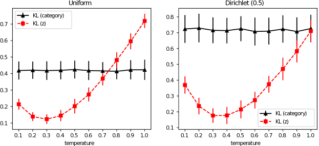
Figure 3: KL divergence between category distributions v.s. KL divergence between corresponding Gumbel distributions ($\bm{y}$) after dimensionality reduction ($\bm{z}$). The figures show mean$\pm$standard deviation of KL. Both of KL divergences are computed by discretizing $(-1,1)$ into $R=100$ intervals.

4 Experimental Results

Table 1: Training and testing errors (estimated variational bound) on the MNIST dataset and the corresponding model configuration. “iconv” consists 5 convolutional layers; “oconv” consists of one RELU layer and 4 transposed convolutional layers.

	Model		$term_{2}$	$\mathcal{L}$	$\gamma$	network shape	$C$	$M$	$R$
$L=1$	Gauss-VAE		80.2	101.3	1e-3	784-400-400-20-400-400-784	$-$	$-$	$-$
	Cat-VAE	T=0.5	86.5	105.8	1e-3	784-400-400-20-400-400-784	5	$-$	$-$
		T=0.8	84.2	101.5	1e-3	784-400-400-20-400-400-784	10	$-$	$-$
	CG-BPEF-VAE	T=0.5	77.8	$\bm{97.4}$	1e-3	784-400-400-20-400-400-784	$-$	5	101
		T=0.8	75.9	$\bm{92.8}$	1e-3	784-400-400-30-400-400-784	$-$	5	101
$L=10$	Gauss-VAE		78.5	100.0	1e-3	784-400-400-20-400-400-784	$-$	$-$	$-$
	Cat-VAE	T=0.5	78.8	98.2	1e-3	784-400-400-20-400-400-784	15	$-$	$-$
		T=0.8	76.9	94.2	1e-3	784-400-400-20-400-400-784	20	$-$	$-$
	CG-BPEF-VAE	T=0.5	74.8	$\bm{94.7}$	1e-3	784-400-400-60-400-400-784	$-$	15	101
		T=0.8	73.2	$\bm{90.4}$	1e-3	784-400-400-40-400-400-784	$-$	5	101

(a) MNIST

	Model		$term_{2}$	$\mathcal{L}$	$\gamma$	network shape	$C$	$M$	$R$
$L=1$	Gauss-VAE		616.3	624.7	1e-3	1024-iconv-128-30-128-oconv-1024	$-$	$-$	$-$
	Cat-VAE	T=0.5	619.5	626.2	1e-3	1024-iconv-128-20-128-oconv-1024	10	$-$	$-$
		T=0.8	617.6	623.7	1e-3	1024-iconv-128-20-128-oconv-1024	10	$-$	$-$
	CG-BPEF-VAE	T=0.5	615.4	$\bm{622.7}$	1e-3	1024-iconv-128-20-128-oconv-1024	$-$	15	101
		T=0.8	613.4	$\bm{620.3}$	1e-3	1024-iconv-128-20-128-oconv-1024	$-$	5	101
$L=10$	Gauss-VAE		615.7	624.4	1e-3	1024-iconv-128-10-128-oconv-1024	$-$	$-$	$-$
	Cat-VAE	T=0.5	616.6	623.2	1e-3	1024-iconv-128-20-128-oconv-1024	15	$-$	$-$
		T=0.8	615.1	620.4	1e-3	1024-iconv-128-20-128-oconv-1024	20	$-$	$-$
	CG-BPEF-VAE	T=0.5	613.4	$\bm{621.6}$	1e-3	1024-iconv-128-20-128-oconv-1024	$-$	10	101
		T=0.8	611.7	$\bm{619.0}$	1e-3	1024-iconv-128-30-128-oconv-1024	$-$	5	101

(b) SVHN

We implemented the proposed method using TensorFlow Abadi, Martín et al. (2015) and tested it on two different datasets. The MNIST dataset LeCun et al. consists of 70,000 gray scale images of hand-written digits, each of size $28\times 28$. The training/validation/testing sets are split according to the ratio $11:1:2$. The SVHN dataset Netzer et al. (2011) has around 100,000 gray-scale pictures (for simplicity the original $32\times 32\times 3$ RGB images are reduced into $32\times 32\times 1$ by averaging the 3 channels) of door numbers with a train/valid/test split of $10:1:3.5$. These pictures are centered by cropping from real street view images.

We only investigate unsupervised density estimation. It is nevertheless meaningful to have unsupervised VAE results on the selected datasets for future references. We compare the proposed CG-BPEF-VAE with vanilla VAE (Gauss-VAE) and Category VAE (Cat-VAE) Jang et al. (2017). For MNIST, the candidate network shapes are 784-400-(10,20,$\cdots$,80)-400-784 and 784-400-400-(10,20,$\cdots$,80)-400-400-784, equipped with densely connected layers and RELU activations Nair & Hinton (2010). For SVHN, the encoder network has 5 convolutional layers with fixed size, reducing the images into a 128-dimensional feature space, and a bottleneck layer of size (10,20,30,40,50) (5 different configurations). The decoder network has one RELU layer of size 128, followed by 4 transposed convolutional layers with fixed size. See the appendix for the detailed configurations.

The learning rate is $\gamma\in\{10^{-4},5\times{}10^{-4},10^{-3},5\times 10^{-3}\}$. For Cat-VAE and CG-BPEF-VAE, the initial and final temperature are $T_{\max}\in\{1,T_{\min}\}$ and $T_{\min}\in\{0.5,0.8\}$, respectively, with a simple exponential annealing scheme. For Cat-VAE, the number of categories is $C\in\{5,10,15,20\}$. For CG-BPEF-VAE, we set the polynomial order $M\in\{5,10,15,20\}$, and the precision $R\in\{51,101\}$. The mini-batch size is fixed to 100. The maximum number of mini-batch iterations is 10,000. For all methods we adopt the Adam optimizer Kingma & Ba (2014) and the Xavier initialization Glorot & Bengio (2010), which are commonly recognized to bring improvements.

The performance is measured by the per-sample average free energy $\mathcal{L}(\bm{\varphi},\bm{\theta})$. The best model with the smallest validated $\mathcal{L}$ is selected. Then the we report its $\mathcal{L}$ on the testing set, along with the reconstruction error $term_{2}$ so that one can tell its trade-off between model complexity ($term_{1}$) and fitness to the data ($term_{2}$). See table 1(b) for the results on two different latent sample size $L$ and two different temperatures $T_{\min}$.

We clearly see that CG-BPEF-VAE shows the best results. Essentially, Gauss-VAE can be considered as a special case of CG-BEPF-VAE when $M=2$ therefore cannot model higher order moments. Cat-VAE has neither a polynomial exponential structure to regulate the discrete variables, nor a dimensionality reduction layer to reduce the free energy. The good results of CG-BPEF-VAE are expected.

Notice that as we increase the final temperature $T_{\min}$, both Cat-VAE and CG-BPEF-VAE will show “better” results. However, the estimation of the free energy will become more and more inaccurate especially for Cat-VAE, whose estimation is a lower bound of the actual free energy by theorem 1 (2). In high temperature, the free energy can be well above its reported $\mathcal{L}$. In contrast, for CG-BPEF-VAE, its estimated $\mathcal{L}$ is an empirical upper bound of the free energy, as long as $T_{\min}$ is set reasonably small ($T=0.5\sim 1$, see fig. 3).

All models prefer deep architectures over shallow ones. There is a significant improvement of Cat-VAE and CG-BPEF-VAE when $L$ is increased from 1 to 10, when Cat-VAE starts to prefer larger category numbers. A large sample size $L$ is required to model complex multimodal distributions and is recommended for Cat-VAE and CG-BPEF-VAE. As the size of the decoder network scales linearly with $L$, one will face significantly higher computation cost during increasing $L$.

As compared to MNIST, SVHN is more difficult to get improved over the baseline results by Gauss-VAE, because its data manifold is much more complex. One has to incorporate supervised information Kingma et al. (2014) to achieve better results.

Cat-VAE and CG-BPEF-VAE are more computational costly than Gauss-VAE. In Cat-VAE, the tensor $\bm{z}$ has a size of $\mathtt{batch~{}size}\times{L}\times{d}\times{}C$. In CG-BPEF-VAE, the tensor $\bm{y}$ have a size of $\mathtt{batch~{}size}\times{L}\times{d}\times{}R$, although this is immediately reduced to $\mathtt{batch~{}size}\times{L}\times{d}$ by the mapping $\bm{y}\to\bm{z}$. A high precision CG-BPEF-VAE or a Cat-VAE with a large category number will multiply the computational time. Our implementation is available at https://github.com/sunk/cgvae.

5 Information Geometry of VAE

This is a relatively separate section. We present a geometric theory which can be useful to uncover the intrinsics of general VAE modeling not limited to the proposed CG-BPEF-VAE, so that one can architect useful VAE models not only based on variational inference, but also along another geometric axis. We also use this geometry to discuss advantages of the proposed CG-BPEF-VAE.

Notice, this geometry is not about the input feature space or the latent space (space of $\bm{x}$ and $\bm{z}$), but about the models (space of $\bm{\theta}$ and $\bm{\varphi}$) or information geometry Amari (2016).

We will consider the cost function $\mathcal{L}(\bm{\theta},\bm{\varphi})$ averaged with respect to i.i.d. observations $\{\bm{x}^{k}\}_{k=1}^{n}$. $term_{1}$ is the average KL divergence between $q(\bm{z}\,|\,\bm{x}^{k})$ and $p(\bm{z})$. Assume that both $p(\bm{z})$ and $q(\bm{z}\,|\,\bm{x}^{k})$ are in the same exponential family $\mathcal{M}(\bm{\varphi})$ so that $p(\bm{z})=\exp(\bm{t}^{\intercal}(\bm{z})\bm{\varphi}^{z}-F(\bm{\varphi}^{z}))$ and $q(\bm{z}\,|\,\bm{x}^{k})=\exp(\bm{t}^{\intercal}(\bm{z})\bm{\varphi}^{k}-F(\bm{\varphi}^{k}))$, where $\bm{t}(\bm{z})$ is a vector of sufficient statistics (for example in CG-BPEF-VAE, $\bm{t}(\bm{z})=(z,z^{2},z^{3},\cdots)$), and $F(\bm{\varphi})$ is a convex cumulant generating function. This $\mathcal{M}(\bm{\varphi})$ is a statistical manifold, i.e., space of probability distributions where $\bm{\varphi}$ serves as a coordinate system. The dual parameters Amari (2016) of $\mathcal{M}(\bm{\varphi})$, which form another coordinate system, are defined by the moments $\bm{\eta}=E(\bm{t}(\bm{z}))=\int p(\bm{z})\bm{t}(\bm{z})\mathrm{d}\bm{z}$. These two coordinate systems can be transformed back and forth by the Legendre transformations $\bm{\eta}=F^{\prime}(\bm{\varphi})$, $\bm{\varphi}=\mathcal{I}^{\prime}(\bm{\eta})$, where $\mathcal{I}$ is Shannon’s information (negative entropy).

By straightforward derivations,

$$term_{1}=\frac{1}{n}\sum_{k=1}^{n}\left[\mathcal{I}(\bm{\eta}^{k})-(\bm{\eta}^{k})^{\intercal}\bm{\varphi}^{z}\right]+F(\bm{\varphi}^{z}).$$

Notice that the prior $p(\bm{z})$ only appears in $term_{1}$ but not in $term_{2}$. We therefore consider a free $p(\bm{z})$ which minimizes $term_{1}$ with $\{\bm{\varphi}^{k}\}_{k=1}^{n}$ fixed. We have

$$\frac{\partial{}term_{1}}{\partial\bm{\varphi}^{z}}=-\frac{1}{n}\sum_{k=1}^{n}\bm{\eta}^{k}+\frac{\partial F(\bm{\varphi}^{z})}{\partial\bm{\varphi}^{z}}=\bm{\eta}^{z}-\frac{1}{n}\sum_{k=1}^{n}\bm{\eta}^{k}.$$

Therefore the optimal $(\bm{\eta}^{z})^{\star}=\frac{1}{n}\sum_{k=1}^{n}\bm{\eta}^{k}$ is the Bregman centroid Nielsen & Nock (2009) of $\{\bm{\varphi}^{k}\}_{k=1}^{n}$. Geometrically, $term_{1}$ is the average divergence between $\bm{\varphi}^{k}$ and the Bregman centroid and therefore measures the $n$-body compactness of $\{\bm{\varphi}^{k}\}_{k=1}^{n}$. We can therefore have a lower bound of $term_{1}$.

Theorem 2.

Given $q(\bm{z}\,|\,\bm{x}^{k})$ in an exponential family $\mathcal{M}(\bm{\varphi})$, if $p(\bm{z})$ is in the same exponential family, then

$$term_{1}\geq\frac{1}{n}\sum_{k=1}^{n}\mathcal{I}\left(\bm{\eta}^{k}\right)-\mathcal{I}\left(\frac{1}{n}\sum_{k=1}^{n}\bm{\eta}^{k}\right)\geq 0,$$ (5)

where the first “=” holds if and only if $\bm{\eta}^{z}=\frac{1}{n}\sum_{k=1}^{n}\bm{\eta}^{k}$. If $p(\bm{z})$ is non-parametric (not constrained by any parametric structure), then

$$term_{1}\geq\frac{1}{n}\sum_{k=1}^{n}\mathcal{I}(\bm{\eta}^{k})-\mathcal{I}(m)\geq 0,$$ (6)

where $m(\bm{z})=\frac{1}{n}\sum_{k=1}^{n}q(\bm{z}\,|\,\bm{x}^{k})$ is a mixture model which is outside $\mathcal{M}(\bm{\varphi})$.

Comparatively, the non-parametric lower bound eq. 6 is smaller than the parametric bound eq. 5. However it needs to compute the entropy of mixture models Nielsen & Sun (2016), which does not have an analytic solution. Essentially, $term_{1}$ is related to the convexity of Shannon information. In standard VAE, $p(\bm{z})$ is fixed to the standard Gaussian distribution, which is not guaranteed to be the Bregman centroid, and does not activate the lower bound in theorem 2. In CG-BPEF-VAE, $term_{1}$ is closer to this bound because $p(\bm{z})$ is set free in our modeling. This hints that as a future work one can directly replace $term_{1}$ with the lower bound stated in theorem 2 to avoid the model selection of $p(\bm{z})$ and to achieve better performance.

Let $\bm{\mu}^{k}=\bm{\mu}(\bm{x}^{k},\bm{\varphi})$ and $\bm{V}^{k}=\bm{V}(\bm{x}^{k},\bm{\varphi})\succ 0$ be the mean and covariance matrix of $q(\bm{z}\,|\,\bm{x}^{k},\bm{\varphi})$, respectively. A Taylor expansion of $\log p(\bm{x}^{k}\,|\,\bm{z},\bm{\theta})$ at $\bm{z}=\bm{\mu}^{k}$ gives

$$term_{2}\approx\frac{1}{n}\sum_{k=1}^{n}\int q(\bm{z}\,|\,\bm{x}^{k},\bm{\varphi})\bigg{[}-\log p(\bm{x}^{k}\,|\,\bm{\mu}^{k},\bm{\theta})$$

$$-(\bm{z}-\bm{\mu}^{k})^{\intercal}\frac{\log p(\bm{x}^{k}\,|\,\bm{z},\bm{\theta})}{\partial\bm{z}}+\frac{1}{2}(\bm{z}-\bm{\mu}^{k})^{\intercal}\mathcal{G}_{\bm{\theta}}(\bm{\mu}^{k})(\bm{z}-\bm{\mu}^{k})\bigg{]}d\bm{z}$$

$$=\frac{1}{n}\sum_{k=1}^{n}\bigg{[}-\log p(\bm{x}^{k}\,|\,\bm{\mu}^{k},\bm{\theta})+\frac{1}{2}tr\left(\mathcal{G}_{\bm{\theta}}(\bm{\mu}^{k})\bm{V}^{k}\right)\bigg{]},$$

where

$$\mathcal{G}_{\bm{\theta}}(\bm{\mu}^{k})=-\frac{\partial^{2}\log p(\bm{x}^{k}\,|\,\bm{z},\bm{\theta})}{\partial\bm{z}^{2}}\bigg{|}_{\bm{z}=\bm{\mu}^{k}}$$

is the observed Fisher information metric (FIM) Amari (2016) wrt $\bm{z}$ depending on $\bm{\theta}$. The approximation is accurate when $q(\bm{z}\,|\,\bm{x}^{k},\bm{\varphi})$ is Gaussian with vanishing centered-moments of order 3 or above.

Assuming the inference network is flexible enough, minimizing $term_{2}$ alone gives $\bm{\mu}^{k}=(\bm{z}^{k})^{\star}$, $\bm{V}^{k}=\bm{0}$, where $(\bm{z}^{k})^{\star}=\operatorname*{arg\,max}_{\bm{z}}\log p(\bm{x}^{k}\,|\,\bm{z},\,\bm{\theta})$ is the maximum likelihood estimation wrt $\bm{x}^{k}$. This $(\bm{z}^{k})^{\star}$ is the latent $\bm{z}$ learned by a plain autoencoder. Hence $term_{2}$ measures a dissimilarity between $q(\bm{z}\,|\,\bm{x}^{k},\bm{\varphi})$ and the Dirac delta distribution $\delta((\bm{z}^{k})^{\star})$. By theorem 2, we get the following approximation of the variational bound.

Corollary 3.

Assume the inference network is flexible enough. Consider a variation of Gaussian VAE, where both $p(\bm{z})$ and $q(\bm{z}\,|\,\bm{x}^{k})$ are free Gaussian distributions. The optimal $\mathcal{L}^{\star}$ is given by

$$\mathcal{L}^{\star}= \min_{\{\bm{\mu}^{k},\bm{V}^{k},\bm{\theta}\}}\frac{1}{n}\sum_{k=1}^{n}\bigg{[}-\log p(\bm{x}^{k}\,|\,\bm{\mu}^{k},\bm{\theta})+\frac{1}{2}tr\left(\mathcal{G}_{\bm{\theta}}(\bm{\mu}^{k})\bm{V}^{k}\right)$$

$$-\frac{1}{2}\log|\bm{V}^{k}|\bigg{]}+\frac{1}{2}\log\left|\overline{\bm{V}^{k}}+\overline{\bm{\mu}^{k}(\bm{\mu}^{k})^{\intercal}}-\overline{\bm{\mu}^{k}}\;(\overline{\bm{\mu}^{k}})^{\intercal}\right|,$$

where “$\overline{\,\cdot\,}$” means averaging over $k=1,\cdots,n$.

Remark 4.

Consider roughly $\bm{V}^{k}\approx\bm{V}$ and $\bm{V}^{z}=\overline{\bm{\mu}^{k}(\bm{\mu}^{k})^{\intercal}}-\overline{\bm{\mu}^{k}}\;(\overline{\bm{\mu}^{k}})^{\intercal}$. The term $\frac{1}{2}tr\left(\mathcal{G}_{\bm{\theta}}(\bm{\mu}^{k})\bm{V}\right)$ helps to shrink $\bm{V}$ towards $\bm{0}$ and lets $\bm{V}$ respect the data manifold encoded in the spectrum of $\mathcal{G}_{\bm{\theta}}(\bm{\mu}^{k})$. The term $-\frac{1}{2}\log|\bm{V}|+\frac{1}{2}\log\left|\bm{V}+\bm{V}_{z}\right|$ enlarges $\bm{V}$ and lets $\bm{V}$ respect the latent manifold of $\{\bm{\mu}^{k}\}$. This reveals a fundamental trade-off between fitting the input data and generalizing.

Remark 5.

In Gaussian VAE with $L=1$, the term $\frac{1}{2}tr\left(\mathcal{G}_{\bm{\theta}}(\bm{\mu}^{k})\bm{V}^{k}\right)$ is inaccurate. Approximating this term can potentially give more effective implementations of VAE.

Remark 6.

Using BPEF for $q(\bm{z}\,|\,\bm{x}^{k},\bm{\varphi})$ has the advantage that the information preserved in higher order differentiations $\frac{\partial^{d}\log p(\bm{x}\,|\,\bm{z},\,\bm{\theta})}{\partial\bm{z}^{d}}$ ($d\geq 3$) is captured.

Figure 4: A geometric picture of VAE learning. $\mathcal{M}(\bm{\varphi})$ is an exponential family with natural parameters $\bm{\varphi}$ to which $p(\bm{z})$ and $q(\bm{z}\,|\,\bm{x}^{k},\bm{\varphi})$ both belong. Learning is to minimize the total “length” of those colored strings.

In summary, fig. 4 presents the information geometric background of VAE on the statistical manifold $\mathcal{M}(\bm{\varphi})$ which includes $p(\bm{z})$, $q(\bm{z}\,|\,\bm{x}^{k})$ and $\delta((\bm{z}^{k})^{\star})$. Note that $\delta((\bm{z}^{k})^{\star})$ is along the boundary of $\mathcal{M}(\bm{\varphi})$, where the variance is 0. For example, a Gaussian distribution $G(\mu,\sigma)$ with $\sigma\to 0$ becomes $\delta(\mu)$. $\{\delta((\bm{z}^{k})^{\star})\}$ vary according to maximum likelihood learning along another statistical manifold $\mathcal{M}(\bm{\theta})$. The cost function $\mathcal{L}$ is interpreted as the geometric compactness of those three sets of distributions. This is essentially related to the theory of minimum description length Hinton & Zemel (1994); Sun et al. (2015).

$\mathcal{G}_{\bm{\theta}}(\bm{z})$ also gives a lower bound (Cramér-Rao bound, Cramér 1946) on the variance of $\bm{z}$, which is given by $\mathcal{G}_{\bm{\theta}}^{-1}(\bm{z})$. In other words, there is a minimum precision (or maximum accuracy) that one can achieve in the inference of $\bm{z}$ given $\bm{x}^{k}$. Although it is hard to compute exactly, it is important to realize the existence of this bound. We give the following rough estimation. Because each $\bm{z}$ has only single observation, the FIM of $\bm{z}$ does not scale with $n$. On the other hand, $\bm{\theta}$ has $n$ repeated observations. Therefore its FIM $\mathcal{G}(\bm{\theta})=\sum_{k=1}^{n}E_{p}\left(-\partial^{2}\log{p}(\bm{x}^{k}\,|\,\bm{z},\bm{\theta})/\partial\bm{\theta}^{2}\right)$ scales linearly with $n$, meaning that the precision of $\bm{\theta}$ scales with $1/\sqrt{n}$. Therefore the precision of $\bm{z}$ is roughly $\sqrt{n}$ times the precision of $\bm{\theta}$. Hence the estimation of $\bm{z}$ should indeed be inaccurate as compared to $\bm{\theta}$. This means that the proposed coarse grain technique is not only for computational convenience, but also has a theoretical background.

6 Concluding Remarks

Within the variational auto-encoding framework Kingma & Welling (2014), this paper proposed a new method CG-BPEF-VAE. Among numerous variations of VAE Burda et al. (2016); Jang et al. (2017), CG-BPEF-VAE is featured by using a universal BPEF density generator in the inference model, and providing a principled way to simulate continuous densities using discrete latent variables. For example, to apply another sophisticated distribution on the latent variable $\bm{z}$, one can employ our CG technique so as to use the reparameterization trick. This study touches a fundamental problem in unsupervised learning: how to build a discrete latent structure to factor information in a continuous representation? We provide preliminary results on unsupervised density estimation, showing performance improvements over the original VAE and category VAE Jang et al. (2017). An empirical study can be extended to semi-supervised learning. This is ongoing work.

We try to picture an information geometric background of VAE. Essentially VAE learns on two manifolds $\mathcal{M}(\bm{\theta})$ and $\mathcal{M}(\bm{\varphi})$, where the cost function can be geometrically interpreted as a sum of divergences within a $n$-body system. This potentially leads to new implementations based on information geometry, e.g., using alternative divergences.

BPEF uses a linear combination of basis distributions in the $\theta$-coordinates (natural parameters). Another basic way to define probability distributions is mixture modeling, or linear combination in the $\eta$-coordinates (moment parameters). The coarse grained technique can be extended to a mixture of BPEF densities, which could more effectively model multi-modal distributions.

Appendix A Proof of Theorem 1

Proof.

We first prove (1). The mapping $z=\bm{y}^{\intercal}\bm{\zeta}$ is from the simplex

$$\Delta^{R-1}=\left\{\bm{y}\in\Re^{R}\,:\,\sum_{i=1}^{R}y_{i}=1;\;\forall{i},y_{i}\geq 0\right\}$$

to the line segment [-1,1]. We therefore define the following subset

$$\mathcal{S}_{z}=\left\{\bm{y}\in\Delta^{R-1}\,:\,\bm{y}^{\intercal}\bm{\zeta}=z\right\}\subset\Delta^{R-1},$$

where $-1\leq{z}\leq 1$. There we have the following partition scheme

$$\Delta^{R-1}=\biguplus_{z=-1}^{1}\mathcal{S}_{z}.$$

Note $\mathrm{KL}(q(\bm{y}\,|\,\bm{x},\bm{\varphi}):p(\bm{y}\,|\,\bm{a}))$ is the KL divergence between two distributions on $\Delta^{R-1}$. By information monotonicity,

$$\mathrm{KL}(q(\bm{y}\,|\,\bm{x},\bm{\varphi})\,:\,p(\bm{y}\,|\,\bm{a}))\geq\mathrm{KL}(q(\mathcal{S}_{z}\,|\,\bm{x},\bm{\varphi})\,:\,p(\mathcal{S}_{z}\,|\,\bm{a})).$$

where $q(\mathcal{S}_{z}\,|\,\bm{x},\bm{\varphi})=\int_{\bm{y}\in\mathcal{S}_{z}}q(\bm{y}\,|\,\bm{x},\bm{\varphi})\mathrm{d}\bm{y}$ and $p(\mathcal{S}_{z}\,|\,\bm{a})=\int_{\bm{y}\in\mathcal{S}_{z}}p(\bm{y}\,|\,\bm{a})\mathrm{d}\bm{y}$ are coarse grained distributions defined on $[-1,1]$, that is, $q(\bm{z}\,|\,\bm{x},\bm{\varphi})$ and $p(\bm{z}\,|\,\bm{a})$.

To prove (2), we partition $\bm{\Delta}^{R-1}$ based on a Voronoi diagram. Let

$$V_{r}=\{\bm{y}\in\Delta^{R-1}\,:\,\|\bm{y}-\bm{e}_{r}\|_{2}\leq\|\bm{y}-\bm{e}_{o}\|,\forall{o}\neq{r}\}.$$

where $\bm{e}_{r}\in\Delta^{R-1}$ has the $r$’th bit set to 1 and the rest bits set to 0. By the basic property of Concrete distribution (Eq.(8) in the paper),

$$\int_{\bm{y}\in{V}_{r}}q(\bm{y}\,|\,\bm{x},\bm{\varphi})\mathrm{d}\bm{y} =P(y_{r}\geq{y}_{o},\forall{o}\neq{r})=\frac{\exp(\beta_{jr})}{\sum_{r=1}^{R}\exp(\beta_{jr})},$$

$$\int_{\bm{y}\in{V}_{r}}p(\bm{y}\,|\,\bm{a})\mathrm{d}\bm{y} =\frac{\exp(\alpha_{jr})}{\sum_{r=1}^{R}\exp(\alpha_{jr})}.$$

Then (2) follows immediately from information monotonicity. ∎

Appendix B Proof of Theorem 2

Lemma 1.

Let $p(\bm{z})=\exp(\bm{\varphi}^{\intercal}\bm{t}(\bm{z})-F(\bm{\varphi}))$ be a distribution in an exponential family , then we have $\mathcal{I}(\bm{\eta})-\bm{\eta}^{\intercal}\bm{\varphi}+F(\bm{\varphi})=0$.

Proof.

By definition,

$$\mathcal{I}(\bm{\eta}) =\int p(\bm{z})\log p(\bm{z})\mathrm{d}z=\int p(\bm{z})\left(\bm{\varphi}^{\intercal}\bm{t}(\bm{z})-F(\bm{\varphi})\right)\mathrm{d}z$$

$$=\bm{\varphi}^{\intercal}\int p(\bm{z})\bm{t}(\bm{z})\mathrm{d}z-F(\bm{\varphi})=\bm{\varphi}^{\intercal}\bm{\eta}-F(\bm{\varphi}).$$

∎

Proof.

If both $q(\bm{z}\,|\,\bm{x}^{k})$ and $p(\bm{z})$ are in the same exponential family, we have

$$p(\bm{z}) =\exp\left(\bm{t}^{\intercal}(\bm{z})\bm{\varphi}^{z}-F(\bm{\varphi}^{z})\right),$$

$$q(\bm{z}\,|\,\bm{x}^{k}) =\exp\left(\bm{t}^{\intercal}(\bm{z})\bm{\varphi}^{k}-F(\bm{\varphi}^{k})\right).$$

Therefore

$$term_{1}= \frac{1}{n}\sum_{k=1}^{n}\mathrm{KL}\left(q(\bm{z}\,|\,\bm{x}^{k},\bm{\varphi})\,:\,p(\bm{z}\,|\,\bm{\varphi}^{z})\right)$$

$$= \frac{1}{n}\sum_{k=1}^{n}\int q(\bm{z}\,|\,\bm{x}^{k},\bm{\varphi})\log\frac{q(\bm{z}\,|\,\bm{x}^{k},\bm{\varphi})}{p(\bm{z}\,|\,\bm{\varphi}^{z})}\mathrm{d}z$$

$$= \frac{1}{n}\sum_{k=1}^{n}\left[\mathcal{I}(\bm{\eta}^{k})-\int q(\bm{z}\,|\,\bm{x}^{k},\bm{\varphi})(\bm{t}^{\intercal}(\bm{z})\bm{\varphi}^{z}-F(\bm{\varphi}^{z}))\mathrm{d}z\right]$$

$$= \frac{1}{n}\sum_{k=1}^{n}\left[\mathcal{I}(\bm{\eta}^{k})-(\bm{\eta}^{k})^{\intercal}(\bm{\varphi}^{z})+F(\bm{\varphi}^{z})\right].$$ (7)

Because $F(\bm{\varphi}^{z})$ is convex with respect to $\bm{\varphi}^{z}$, setting its derivative

$$\frac{\partial{term_{1}}}{\partial\bm{\varphi}^{z}}=\frac{1}{n}\sum_{k=1}^{n}\left[-\bm{\eta}^{k}+\frac{\partial F}{\partial\bm{\varphi}^{z}}\right]=\frac{1}{n}\sum_{k=1}^{n}\left[-\bm{\eta}^{k}+\bm{\eta}^{z}\right]\quad\text{(Legendre transformation)}$$

to zero gives the unique minimizer of $term_{1}$:

$$(\bm{\eta}^{z})^{\star}=\frac{1}{n}\sum_{k=1}^{n}\bm{\eta}^{k}.$$

Plugging this into Eq. B, we get

$$term_{1}^{\star} =\frac{1}{n}\sum_{k=1}^{n}\left[\mathcal{I}(\bm{\eta}^{k})-(\bm{\eta}^{k})^{\intercal}(\bm{\varphi}^{z})^{\star}+F((\bm{\varphi}^{z})^{\star})\right]$$

$$=\frac{1}{n}\sum_{k=1}^{n}\left[\mathcal{I}(\bm{\eta}^{k})-((\bm{\varphi}^{z})^{\star})^{\intercal}\bm{\eta}^{k}+((\bm{\varphi}^{z})^{\star})^{\intercal}(\bm{\eta}^{z})^{\star}-\mathcal{I}((\bm{\eta}^{z})^{\star})\right]\quad\text{(by the Lemma)}$$

$$=\frac{1}{n}\sum_{k=1}^{n}\mathcal{I}(\bm{\eta}^{k})-((\bm{\varphi}^{z})^{\star})^{\intercal}\frac{1}{n}\sum_{k=1}^{n}\bm{\eta}^{k}+((\bm{\varphi}^{z})^{\star})^{\intercal}(\bm{\eta}^{z})^{\star}-\mathcal{I}((\bm{\eta}^{z})^{\star})$$

$$=\frac{1}{n}\sum_{k=1}^{n}\mathcal{I}(\bm{\eta}^{k})-\mathcal{I}\left(\frac{1}{n}\sum_{k=1}^{n}\bm{\eta}^{k}\right).$$

By the above analysis, $term_{1}\geq term_{1}^{\star}$, and the “=” holds if and only if $\bm{\eta}^{z}=(\bm{\eta}^{z})^{\star}$. The second “$\geq$” is straightforward from the fact that $\mathcal{I}$ is a convex function in the coordinate system $\bm{\eta}$.

If $p(\bm{z})$ is non-parametric, then

$$term_{1}= \frac{1}{n}\sum_{k=1}^{n}\int q(\bm{z}\,|\,\bm{x}^{k},\bm{\varphi})\log\frac{q(\bm{z}\,|\,\bm{x}^{k},\bm{\varphi})}{p(\bm{z}\,|\,\bm{\varphi}^{z})}\mathrm{d}z$$

$$= \frac{1}{n}\sum_{k=1}^{n}\left[\mathcal{I}(\bm{\eta}^{k})-\int q(\bm{z}\,|\,\bm{x}^{k},\bm{\varphi})\log p(\bm{z}\,|\,\bm{\varphi}^{z})\mathrm{d}z\right]$$

$$= \frac{1}{n}\sum_{k=1}^{n}\mathcal{I}(\bm{\eta}^{k})-\int\frac{1}{n}\sum_{k=1}^{n}q(\bm{z}\,|\,\bm{x}^{k},\bm{\varphi})\log p(\bm{z}\,|\,\bm{\varphi}^{z})\mathrm{d}z.$$ (8)

Therefore, $term_{1}$ is minimized at $p(\bm{z}\,|\,(\bm{\varphi}^{z})^{\star})=\frac{1}{n}\sum_{k=1}^{n}q(\bm{z}\,|\,\bm{x}^{k},\bm{\varphi})$. Plugging this minimizer into the above Eq. B, we get

$$term_{1}^{\star}=\frac{1}{n}\sum_{k=1}^{n}\mathcal{I}(\bm{\eta}^{k})-\int\frac{1}{n}\sum_{k=1}^{n}q(\bm{z}\,|\,\bm{x}^{k},\bm{\varphi})\log\left[\frac{1}{n}\sum_{k=1}^{n}q(\bm{z}\,|\,\bm{x}^{k},\bm{\varphi})\right]\mathrm{d}z.$$

Note that the mixture model $\frac{1}{n}\sum_{k=1}^{n}q(\bm{z}\,|\,\bm{x}^{k},\bm{\varphi})$ is outside the exponential family $\mathcal{M}(\bm{\varphi})$. ∎

Appendix C The Effect of the Dimensionality Reduction Layer of CG-BPEF-VAE

Fig. 5 shows the $\mathrm{KL}(p(\bm{z}):\mathtt{Uniform})$ (KL(z)) and $\mathrm{KL}(\bm{\alpha}:\mathtt{Uniform})$ (KL(category)) when $\bm{\alpha}$ is generated by Dirichlet distributions with different configurations. In all cases, $\mathrm{KL}(\bm{\alpha}:\mathtt{Uniform})$ is lower bounded by $\mathrm{KL}(p(\bm{z}):\mathtt{Uniform})$ for small temperature.

Appendix D Visualization of the Concrete Distribution

Fig. 6, Fig. 7 and Fig. 8 show Concrete densities generated by random sampling. For each experiment (sub-figure), we generate $10^{6}$ Concrete samples and plot the resulting density. There are very high density regions near the corner (the red region), which are cropped so that the visualization is clear.

An interesting observation is that the density will “leak” to the simplex faces if $T$ is small, although in this case the density will concentrate on the corners. Therefore it may not always be good to choose a small $T$. This is ongoing study.

Appendix E Details of the Convolutional Layers

We used convolutional layers on the SVHN dataset. The encoder is specified by

• Input: $1\times 32\times 32$ (RGB is averaged into 1 channel)

• Convolutional layer: 32 ($5\times 5$) filters, with ReLU activation and no padding
  ($\to 32\times 28\times 28$)

• Pooling layer: $2\times 2$ filter with a stride of 2 and no padding zeros
  ($\to 32\times 14\times 14$)

• Convolutional layer: 64 ($5\times 5$) filters, with ReLU activation and no padding
  ($\to 64\times 10\times 10$)

• Pooling layer: $2\times 2$ filter with a stride of 2 and no padding
  ($\to 64\times 5\times 5$)

• Convolutional layer: 128 ($5\times 5$) filters, with RELU activation and no padding
  ($\to 128\times 1\times 1$)

The decoder is specified by

• A dense linear layer with RELU activation to transform the dimension to 128

• Transposed convolutional layer: 64 ($5\times 5$) filters with stride 4; with RELU activation
  ($\to 64\times 4\times 4$)

• Transposed convolutional layer: 32 ($5\times 5$) filters with stride 2; with RELU activation
  ($\to 32\times 8\times 8$)

• Transposed convolutional layer: 16 ($5\times 5$) filters with stride 2; with RELU activation
  ($\to 16\times 16\times 16$)

• Transposed convolutional layer: 1 ($5\times 5$) filters with stride 2; without non-linear activation
  ($\to 1\times 32\times 32$)

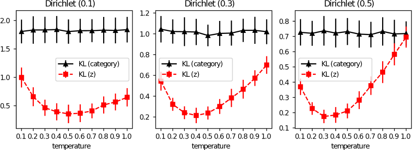
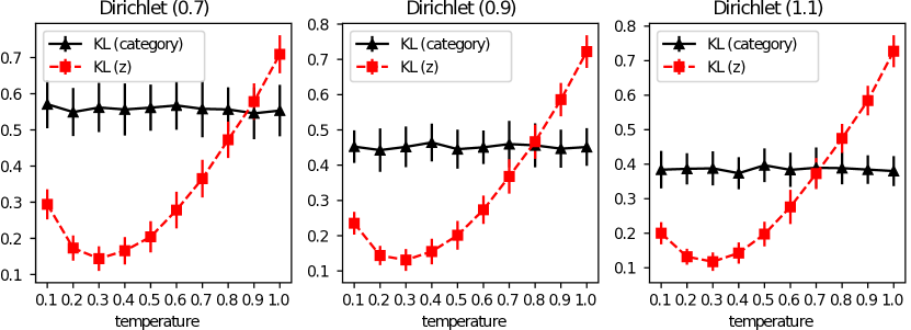
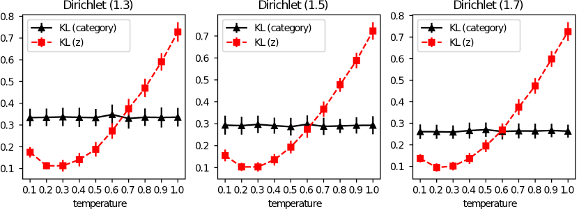
Figure 5: KL divergence between category distributions v.s. KL divergence between corresponding Gumbel distributions ($\bm{y}$) after dimensionality reduction ($\bm{z}$). The figures show mean$\pm$standard deviation of KL. Both of KL divergences are computed by discretizing $(-1,1)$ into $R=100$ intervals.

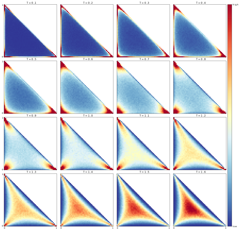
Figure 6: The density of $\mathrm{Con}(\bm{\alpha},T)$, where $\bm{\alpha}=(1/3,1/3,1/3)$ and $T=0.1,0.2,\cdots,1.6$ (from left to right, from top to bottom). Best viewed in color.

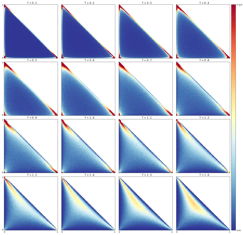
Figure 7: The density of $\mathrm{Con}(\bm{\alpha},T)$, where $\bm{\alpha}=(1/2,1/3,1/6)$ and $T=0.1,0.2,\cdots,1.6$ (from left to right, from top to bottom). Best viewed in color.

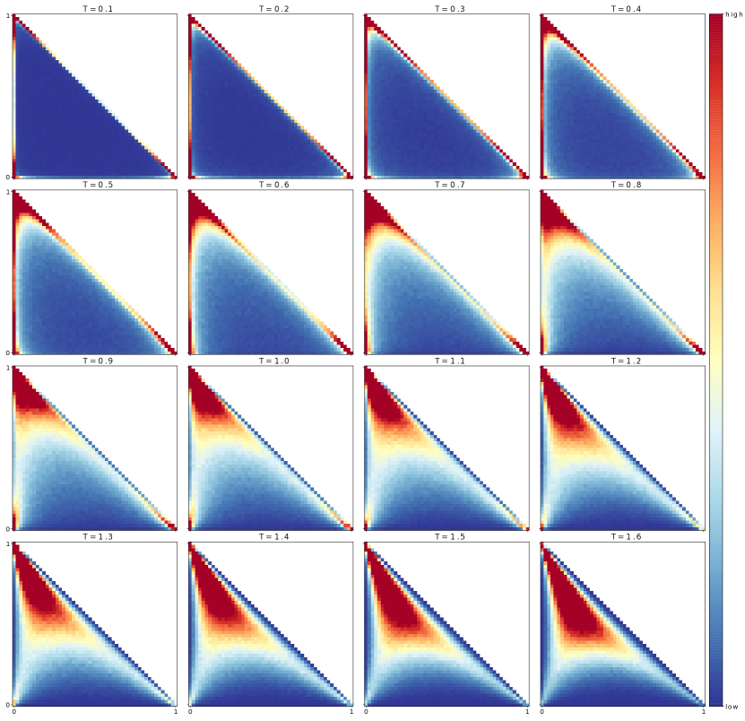
Figure 8: The density of $\mathrm{Con}(\bm{\alpha},T)$, where $\bm{\alpha}=(2/3,1/6,1/6)$ and $T=0.1,0.2,\cdots,1.6$ (from left to right, from top to bottom). Best viewed in color.

References

- Abadi, Martín et al. (2015) Abadi, Martín et al. TensorFlow: Large-scale machine learning on heterogeneous systems, 2015. Software available from tensorflow.org.
- Amari (2016) Amari, Shun-ichi. Information Geometry and its Applications, volume 194 of Applied Mathematical Sciences. Springer Japan, 2016.
- Burda et al. (2016) Burda, Yuri, Grosse, Roger, and Salakhutdinov, Ruslan. Importance weighted autoencoders. In ICLR, 2016. arXiv:1509.00519 [cs.LG].
- Cobb et al. (1983) Cobb, Loren, Koppstein, Peter, and Chen, Neng Hsin. Estimation and moment recursion relations for multimodal distributions of the exponential family. Journal of the American Statistical Association, 78(381):124–130, 1983.
- Cramér (1946) Cramér, Harald. Mathematical Methods of Statistics, volume 9 of Princeton Mathematical Series. Princeton University Press, 1946.
- de Haan & Ferreira (2006) de Haan, Laurens and Ferreira, Ana. Extreme Value Theory: An Introduction. Springer Series in Operations Research and Financial Engineering. Springer-Verlag New York, 2006.
- Dilokthanakul et al. (2017) Dilokthanakul, Nat, Mediano, Pedro A.M., Garnelo, Marta, Lee, Matthew C.H., Salimbeni, Hugh, Arulkumaran, Kai, and Shanahan, Murray. Deep unsupervised clustering with Gaussian mixture variational autoencoders. In ICLR, 2017. arXiv:1611.02648 [cs.LG].
- Glorot & Bengio (2010) Glorot, Xavier and Bengio, Yoshua. Understanding the difficulty of training deep feedforward neural networks. In AISTATS; JMLR W&CP 9, pp. 249–256, 2010.
- Gregor et al. (2015) Gregor, Karol, Danihelka, Ivo, Graves, Alex, Rezende, Danilo Jimenez, and Wierstra, Daan. DRAW: A recurrent neural network for image generation. In ICML; JMLR W & CP 37, pp. 1462–1471, 2015.
- Gumbel (1954) Gumbel, Emil Julius. Statistical theory of extreme values and some practical applications: a series of lectures. Applied mathematics series. U. S. Govt. Print. Office, 1954.
- Hinton & Zemel (1994) Hinton, Geoffrey E and Zemel, Richard S. Autoencoders, minimum description length and Helmholtz free energy. In NIPS 6, pp. 3–10. Morgan-Kaufmann, 1994.
- Jang et al. (2017) Jang, Eric, Gu, Shixiang, and Poole, Ben. Categorical reparameterization with Gumbel-softmax. In ICLR, 2017. arXiv:1611.01144 [stat.ML].
- Jordan et al. (1999) Jordan, Michael I., Ghahramani, Zoubin, Jaakkola, Tommi S., and Saul, Lawrence K. An introduction to variational methods for graphical models. Machine Learning, 37(2):183–233, 1999.
- Kingma & Ba (2014) Kingma, Diederik P. and Ba, Jimmy. Adam: A method for stochastic optimization. CoRR, abs/1412.6980, 2014.
- Kingma & Welling (2014) Kingma, Diederik P and Welling, Max. Auto-encoding variational Bayes. In ICLR, 2014. arXiv:1312.6114 [stat.ML].
- Kingma et al. (2014) Kingma, Diederik P, Mohamed, Shakir, Jimenez Rezende, Danilo, and Welling, Max. Semi-supervised learning with deep generative models. In NIPS 27, pp. 3581–3589. Curran Associates, Inc., 2014.
- Kuzmin & Warmuth (2005) Kuzmin, Dima and Warmuth, Manfred K. Optimum follow the leader algorithm. In COLT, pp. 684–686, 2005.
- (18) LeCun, Yann, Cortes, Corinna, and Burges, Christopher J.C. The MNIST database of handwritten digits. URL http://yann.lecun.com/exdb/mnist/.
- Maddison et al. (2014) Maddison, Chris J, Tarlow, Daniel, and Minka, Tom. A sampling. In NIPS 27, pp. 3086–3094. Curran Associates, Inc., 2014.
- Maddison et al. (2016) Maddison, Chris J., Mnih, Andriy, and Teh, Yee Whye. The Concrete distribution: A continuous relaxation of discrete random variables. CoRR, abs/1611.00712, 2016. to be presented in ICLR 2017.
- Nair & Hinton (2010) Nair, V. and Hinton, G. E. Rectified linear units improve restricted Boltzmann machines. In ICML, pp. 807–814, 2010.
- Netzer et al. (2011) Netzer, Yuval, Wang, Tao, Coates, Adam, Bissacco, Alessandro, Wu, Bo, and Ng, Andrew Y. Reading digits in natural images with unsupervised feature learning. In NIPS Workshop on Deep Learning and Unsupervised Feature Learning, 2011. URL http://ufldl.stanford.edu/housenumbers.
- Nielsen & Nock (2009) Nielsen, Frank and Nock, Richard. Sided and symmetrized Bregman centroids. IEEE Transactions on Information Theory, 55(6):2882–2904, 2009.
- Nielsen & Nock (2016) Nielsen, Frank and Nock, Richard. Patch matching with polynomial exponential families and projective divergences. In International Conference on Similarity Search and Applications (SISAP), pp. 109–116, 2016.
- Nielsen & Sun (2016) Nielsen, Frank and Sun, Ke. Guaranteed bounds on information-theoretic measures of univariate mixtures using piecewise log-sum-exp inequalities. Entropy, 18(12):442, 2016.
- Rezende et al. (2014) Rezende, Danilo Jimenez, Mohamed, Shakir, and Wierstra, Daan. Stochastic backpropagation and approximate inference in deep generative models. In ICML; JMLR W&CP 32 (2), pp. 1278–1286, 2014.
- Salimans et al. (2015) Salimans, Tim, Kingma, Diederik, and Welling, Max. Markov chain Monte Carlo and variational inference: Bridging the gap. In ICML; JMLR W&CP 37, pp. 1218–1226, 2015.
- Serban et al. (2016) Serban, Iulian Vlad, II, Alexander G. Ororbia, Pineau, Joelle, and Courville, Aaron C. Multi-modal variational encoder-decoders. CoRR, abs/1612.00377, 2016.
- Shu, Rui et al. (2016) Shu, Rui et al. Stochastic video prediction with conditional density estimation. In ECCV Workshop on Action and Anticipation for Visual Learning, 2016.
- Sohn et al. (2015) Sohn, Kihyuk, Lee, Honglak, and Yan, Xinchen. Learning structured output representation using deep conditional generative models. In NIPS 28, pp. 3483–3491. Curran Associates, Inc., 2015.
- Sun et al. (2015) Sun, Ke, Wang, Jun, Kalousis, Alexandros, and Marchand-Maillet, Stéphane. Information geometry and minimum description length networks. In ICML; JMLR W&CP 37, pp. 49–58, 2015.
- Walker et al. (2016) Walker, Jacob, Doersch, Carl, Gupta, Abhinav, and Hebert, Martial. An uncertain future: Forecasting from static images using variational autoencoders. In ECCV; LNCS 9911, pp. 835–851, 2016.