Triple Regge exchange mechanisms
of four-pion continuum production
in the $pp\to pp\pi^{+}\pi^{-}\pi^{+}\pi^{-}$ reaction

Abstract

We consider exclusive multi-peripheral production of four charged pions in proton-proton collisions at high energies with simultaneous exchange of three pomerons/reggeons. The amplitude(s) for the genuine $2\to 6$ process are written in the Regge approach. The calculation is performed with the help of the GenEx Monte Carlo code. Some corrections at low invariant masses in the two-body subsystems are necessary for application of the Regge formalism. We estimate the corresponding cross section and present differential distributions in rapidity, transverse momenta and two- and four-pion invariant masses. The cross section and the distributions depend on the value of the cut-off parameter of a form factor correcting amplitudes for off-shellness of $t$-channel pions. Rather large cross section is found for the whole phase space ($\sigma\sim$ 1-5 $\mu$b, including absorption corrections). Relatively large four-pion invariant masses are populated in the considered diffractive mechanism compared to other mechanisms discussed so far in the context of four-pion production. We investigate whether the triple Regge exchange processes could be identified with the existing LHC detectors. We consider the case of ATLAS and ALICE cuts. The ATLAS (or CMS) has better chances to identify the process in the region of large invariant masses $M_{4\pi}>10$ GeV. In the case of the ALICE experiment the considered mechanism competes with other mechanisms (production of $\sigma\sigma$, $\rho\rho$ pairs or single resonances) and cannot be unambiguously identified.

I Introduction

In the present paper, we study the exclusive $2\to 6$ process:

$$pp\to pp\pi^{+}\pi^{-}\pi^{+}\pi^{-}\,.$$ (1)

In general, the number of possible mechanisms is rather large. Here we shall focus on the triple-Regge exchange processes. According to our knowledge such processes were not discussed quantitatively in the literature and estimation of their importance becomes timely in the light of studies being performed by the STAR, ATLAS, CMS and ALICE collaborations. At the LHC the energy is so high that there is enough rapidity span for such processes to occur, at least from the theoretical point of view.

In this study we present an extension of the Regge-inspired Lebiedowicz-Szczurek approach used for the reactions: $pp\to pp\pi^{+}\pi^{-}$ LS_2pi , LSSTC_2pi , $pp\to nn\pi^{+}\pi^{+}$ LS_nnpipi and $pp\to ppK^{+}K^{-}$ LS_2K . The number of diagrams for the six-body reactions is bigger than for the four-body reaction and we have to carefully write the corresponding amplitudes using, however, simplified Regge rules for $\pi p$ and $\pi\pi$ interactions.

We shall try to use the same model parameters as for the $pp\to pp\pi^{+}\pi^{-}$ whenever possible. This should allow for an approximate estimation of the cross section and some differential distributions. The calculation presented here is performed with the help of the GenEx Monte Carlo event generator GenEx .

We wish to concentrate on the four charged pion continuum production mechanism which, in addition, is a background for studies of central exclusive production of resonances discussed recently in LNS2016_2pi . The production of glueball states is expected to be enhanced in gluon rich pomeron-pomeron interactions. Identification of diffractively produced glueball states is still an experimental challenge at the LHC. For experimental point of view at lower energies see e.g. ABCDHW_4pi . This requires calculation/estimation of the four-pion background from different sources, see e.g. LNS2016_4pi .

II Amplitude for the four-pion continuum production

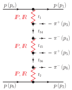
Figure 1: A diagram for exclusive diffractive production of $\pi^{+}\pi^{-}\pi^{+}\pi^{-}$ continuum with three pomeron/reggeon exchanges in proton-proton collisions. Here $\mathbb{R}$ denotes the $f_{2\mathbb{R}}$ or $\rho_{\mathbb{R}}$ reggeon exchanges. The four-momentum transfers squared are shown explicitly.

The general situation for the $pp\to pp\pi^{+}\pi^{-}\pi^{+}\pi^{-}$ process is sketched in Fig. 1. The full amplitude, including different permutations of outgoing pion pairs, can be written as

$$\begin{split}{\cal M}&=\frac{1}{2}\left({\cal M}_{\{3456\}}+{\cal M}_{\{5436\}}+{\cal M}_{\{3654\}}+{\cal M}_{\{5634\}}\right)\\ &+\frac{1}{2}\left({\cal M}_{\{4356\}}+{\cal M}_{\{4536\}}+{\cal M}_{\{6354\}}+{\cal M}_{\{6534\}}\right)\\ &+\frac{1}{2}\left({\cal M}_{\{3465\}}+{\cal M}_{\{5463\}}+{\cal M}_{\{3645\}}+{\cal M}_{\{5643\}}\right)\\ &+\frac{1}{2}\left({\cal M}_{\{4365\}}+{\cal M}_{\{4563\}}+{\cal M}_{\{6345\}}+{\cal M}_{\{6543\}}\right)\,,\end{split}$$ (2)

where the factor $\frac{1}{2}$ is the symmetry factor for two identical pions.

In formulae below the subsystem energies squared is

$$s_{ij}=M_{ij}^{2}=(p_{i}+p_{j})^{2}\,,$$ (3)

where $p_{i}$ and $p_{j}$ are respective four-vectors, and the formulae of four-momentum transfers squared are

$$\begin{split}&t_{1}=(p_{a}-p_{1})^{2}\,,\\ &t_{2}=(p_{b}-p_{2})^{2}\,,\\ &t_{34}=(p_{a}-p_{1}-p_{3})^{2}\,,\\ &t_{43}=(p_{a}-p_{1}-p_{4})^{2}\,,\\ &t_{45}=t_{35}=t_{46}=t_{36}=(p_{a}-p_{1}-p_{3}-p_{4})^{2}=(p_{b}-p_{2}-p_{6}-p_{5})^{2}\;,\\ &t_{56}=(p_{b}-p_{2}-p_{6})^{2}\,,\\ &t_{65}=(p_{b}-p_{2}-p_{5})^{2}\,.\end{split}$$ (4)

We write the amplitude for each group in Eq. (2):

$${\cal M}_{\{3456\}} = A_{\pi p}(s_{13},t_{1})\,\frac{F_{\pi}(t_{34})}{t_{34}-m_{\pi}^{2}}\,A_{\pi\pi}(s_{45},t_{45})\,\frac{F_{\pi}(t_{56})}{t_{56}-m_{\pi}^{2}}\,A_{\pi p}(s_{26},t_{2})\,,$$ (5)

$${\cal M}_{\{4356\}} = A_{\pi p}(s_{14},t_{1})\,\frac{F_{\pi}(t_{43})}{t_{43}-m_{\pi}^{2}}\,A_{\pi\pi}(s_{35},t_{35})\,\frac{F_{\pi}(t_{56})}{t_{56}-m_{\pi}^{2}}\,A_{\pi p}(s_{26},t_{2})\,,$$ (6)

$${\cal M}_{\{3465\}} = A_{\pi p}(s_{13},t_{1})\,\frac{F_{\pi}(t_{34})}{t_{34}-m_{\pi}^{2}}\,A_{\pi\pi}(s_{46},t_{46})\,\frac{F_{\pi}(t_{65})}{t_{65}-m_{\pi}^{2}}\,A_{\pi p}(s_{25},t_{2})\,,$$ (7)

$${\cal M}_{\{4365\}} = A_{\pi p}(s_{14},t_{1})\,\frac{F_{\pi}(t_{43})}{t_{43}-m_{\pi}^{2}}\,A_{\pi\pi}(s_{36},t_{36})\,\frac{F_{\pi}(t_{65})}{t_{65}-m_{\pi}^{2}}\,A_{\pi p}(s_{25},t_{2})\,.$$ (8)

The subprocess amplitudes with the Regge exchanges are given as

$$A_{\pi p}(s,t)=\sum_{j=\mathbb{P},f_{2\mathbb{R}}}\eta_{j}\,s\,C_{\pi p}^{j}\left(\frac{s}{s_{0}}\right)^{\alpha_{j}(t)-1}F_{\pi p}^{j}(t)\,,$$ (9)

$$A_{\pi\pi}(s,t)=\sum_{j=\mathbb{P},f_{2\mathbb{R}}}\eta_{j}\,s\,C_{\pi\pi}^{j}\left(\frac{s}{s_{0}}\right)^{\alpha_{j}(t)-1}F_{\pi\pi}^{j}(t)\,,$$ (10)

where the signature factors at $t=0$ are $\eta_{\mathbb{P}}=i$ and $\eta_{f_{2\mathbb{R}}}=i-0.86$ LS_2pi . The interaction strength parameters are assumed to fulfil the Regge factorization relation:

$$C_{pp}^{j}C_{\pi\pi}^{j}=C_{\pi p}^{j}C_{\pi p}^{j}\,,$$ (11)

where $j=\mathbb{P},f_{2\mathbb{R}}$. In our calculations we use the following numerical parameters

$$C_{pp}^{\mathbb{P}}=21.70\;{\rm mb}\,,\quad C_{\pi p}^{\mathbb{P}}=13.63\;{\rm mb}\,,\quad C_{\pi\pi}^{\mathbb{P}}=8.56\;{\rm mb}\,,$$ (12)

$$C_{pp}^{f_{2\mathbb{R}}}=75.4875\;{\rm mb}\,,\quad C_{\pi p}^{f_{2\mathbb{R}}}=31.79\;{\rm mb}\,,\quad C_{\pi\pi}^{f_{2\mathbb{R}}}=13.39\;{\rm mb}\,.$$ (13)

We parametrize the $t$-dependences of subprocess amplitudes in the exponential form:

$$F_{\pi p}^{j}(t) = \exp\left(\frac{B_{\pi p}^{j}}{2}t\right)\,,$$ (14)

$$F_{\pi\pi}^{j}(t) = \exp\left(\frac{B_{\pi\pi}^{j}}{2}t\right)\,,$$ (15)

where the slope parameters are taken as $B_{\pi p}^{\mathbb{P}}=5.5$ GeV^-2, $B_{\pi\pi}^{\mathbb{P}}=4$ GeV^-2, $B_{\pi p}^{f_{2\mathbb{R}}}=4$ GeV^-2, $B_{\pi\pi}^{f_{2\mathbb{R}}}=4$ GeV^-2 (see LS_2pi ).

The Regge trajectories $\alpha_{j}(t)$ are assumed to be of the standard linear form DDLN :

$$\alpha_{j}(t)=\alpha_{j}(0)+\alpha^{\prime}_{j}t\,,$$ (16)

$$\alpha_{\mathbb{P}}(0)=1.0808\,,\quad\alpha^{\prime}_{\mathbb{P}}=0.25\;{\rm GeV^{-2}}\,,$$ (17)

$$\alpha_{f_{2\mathbb{R}}}(0)=0.5475\,,\quad\alpha^{\prime}_{f_{2\mathbb{R}}}=0.9\;{\rm GeV^{-2}}\,.$$ (18)

The off-shellness of $t$-channel pions in the diagrams is included via multiplication of corresponding amplitudes by the extra form factor:

$$F_{\pi}(t)=\exp\left(\frac{t-m_{\pi}^{2}}{\Lambda_{off,E}^{2}}\right)=\exp\left(\frac{t-m_{\pi}^{2}}{2\Lambda_{off,E}^{2}}\right)\exp\left(\frac{t-m_{\pi}^{2}}{2\Lambda_{off,E}^{2}}\right)\,.$$ (19)

In fact the off-shell effects are related to vertices and they always go in pairs for our process. The form factor is normalized to unity when meson is on-mass-shell $F_{\pi}(m_{\pi}^{2})=1$. The parameter of the off-shell form factor(s) is in principle a free parameter. In the present paper we shall use $\Lambda_{off,E}=1$ GeV (lower limit) and use $\Lambda_{off,E}=1.5$ GeV (upper limit). These values correspond to $\tilde{\Lambda}_{off,E}=1.41$ GeV and $\tilde{\Lambda}_{off,E}=2.12$ GeV in the convention used in LS_2pi .

The amplitudes (9) and (10) have to be corrected (cut off) for low $\sqrt{s_{ij}}=W_{ij}$ as the Regge theory is valid only above a lower subenergy limit. In our analysis here mainly a smooth cut-off function will be used, as in LS_2pi , e.g.,

$$f_{cont}(W_{ij})=\frac{\exp\left((W_{ij}-W_{0})/a\right)}{1+\exp\left((W_{ij}-W_{0})/a\right)},$$ (20)

with $a=0.2$ GeV and $W_{0}=2$ GeV, which cuts off $s_{ij}\lesssim 4$ GeV² smoothly.

Another cut-off function which we use is the Heaviside theta function:

$$f_{discont}(W_{ij})=\theta(W_{ij}-W_{cut}),$$ (21)

where $W_{cut}$ is a parameter to be adjusted to future precise data. We will show that both functions, see (20) and (20), give similar results for the integrated cross section, however, somewhat different distributions in some special variables.

III Feasibility study for the measurement of the triple Regge exchange process at current LHC experiments

In this section we show some predictions for the considered process. We will select $\sqrt{s}=7$ TeV collision energy as a representative example. The collision energy dependence of the cross section is rather weak (see section IV.5).

Presentation of our results is divided into three parts:
(A) calculation for the full six-body phase space,
(B) calculation relevant for the ATLAS main tracker,
(C) calculation relevant for the ALICE main tracker.

In a separate section we discuss some general specific aspects of the discussed here mechanism.

Some technical details related to the Monte Carlo integration are described in Appendix A.

III.1 Results for the full phase space

In this subsection we present some results for cross section calculation which we call "full phase space" meaning that only minimal cuts are imposed for purely technical reasons, namely

$$p_{t,p}<2\;{\rm GeV}\,,\quad|y_{4\pi}|<6\,,\quad M_{4\pi}<30{\rm~{}GeV}.$$ (22)

These cuts can be easily placed in experimental analyses and do not change the shape of the resulting distributions. The condition $M_{4\pi}<30{\rm~{}GeV}$ cuts off less than a few percent of the cross section.

Table 1: Full phase space cross sections in $\mu$b. No absorption effects are included here.

	$\Lambda_{off,E}$ [GeV]	$\sigma$ [$\mu$b]
Symmetrization	1.0	7.21
No symmetrization	1.0	0.82
Symmetrization	1.5	42.86
No symmetrization	1.5	4.30

In Tab. 1 we present numerical results for the cross section integrated over so-defined full phase space. In the table, ’No symmetrization’ means that we take only one arbitrarily chosen term for the matrix element and omit the symmetrization factor, that is, ${\cal M}={\cal M}_{\{3456\}}$ in Eq. (2).

In Figs. 2, 3, 4 and 7 the general features of the investigated process are presented while Figs. 5 and 6 illustrate relative contributions of the pomeron and subleading reggeon trajectories to the calculated cross sections.

The distribution in four-pion invariant mass, see Fig. 3, extends in relatively broad range, compared e.g. to dipion invariant mass distribution for the $pp\to pp\pi^{+}\pi^{-}$ reaction. The four momentum transfer from both protons to the $4\pi$ system is restricted by peripherality of the process what results in relatively narrow distribution of (26) shown in Fig. 21.

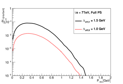
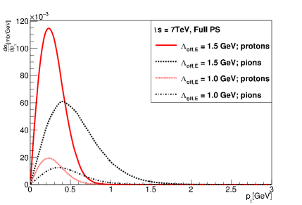
Figure 2: Distributions in transverse momentum of the four-pion system(left panel) and for the transverse momenta of individual particles (protons and pions) for two different values of $\Lambda_{off,E}$ = 1, 1.5 GeV.

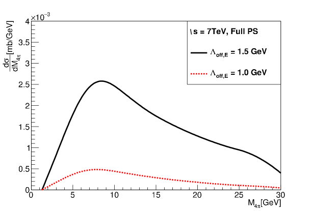
Figure 3: Four-pion invariant mass distribution for the full phase space for two different values of $\Lambda_{off,E}$ = 1, 1.5 GeV.

At $\sqrt{s}=7$ TeV the outgoing protons are produced at $y\approx\pm 9$ (see Fig. 4). The pions are produced between protons. The pion rapidity distribution illustrates well the role of subleading $f_{2\mathbb{R}}$ reggeons. In Fig. 5 we compare distributions for $(\mathbb{P}+f_{2\mathbb{R}})\times(\mathbb{P}+f_{2\mathbb{R}})\times(\mathbb{P}+f_{2\mathbb{R}})$ and $\mathbb{P}\times\mathbb{P}\times\mathbb{P}$ exchanges. Here the notation corresponds to external $\times$ internal $\times$ external exchanges (see Fig. 1). Adding $f_{2\mathbb{R}}$ exchange not only enhances the cross section but also modifies the shape of the distribution. One can observe now clear enhancements at $y\approx\pm 6$ that correspond to the external exchanges of $f_{2\mathbb{R}}$ reggeons. This figure reminds a similar figure for the $pp\to pp\pi^{+}\pi^{-}$ reaction, where a camel-like distribution was obtained LS_2pi . There the peaks at large rapidities correspond to $f_{2\mathbb{R}}$ reggeon exchanges. Here (for the $pp\to pp\pi^{+}\pi^{-}\pi^{+}\pi^{-}$ reaction) three peaks can be observed. In addition, we plot $(\mathbb{P}+f_{2\mathbb{R}})\times f_{2\mathbb{R}}\times(\mathbb{P}+f_{2\mathbb{R}})$ when in the middle only $f_{2\mathbb{R}}$ is present. The cross section is significantly smaller, which means that $\mathbb{P}$ in the middle of the diagram is responsible for the cross section enhancement. There is a qualitative hydromechanical analogy in which all outgoing particles in diagrams (shown schematically in Fig. 1) are represented as liquid layers which move with parallel velocities and protons are the top and bottom layers. Then the coupling/friction between layers is given by the parameters of the pomeron/reggeon exchanges. In Fig. 6, $M_{4\pi}$ distributions for $(\mathbb{P}+f_{2\mathbb{R}})\times(\mathbb{P}+f_{2\mathbb{R}})\times(\mathbb{P}+f_{2\mathbb{R}})$, $\mathbb{P}\times\mathbb{P}\times\mathbb{P}$ and $(\mathbb{P}+f_{2\mathbb{R}})\times f_{2\mathbb{R}}\times(\mathbb{P}+f_{2\mathbb{R}})$ are plotted. We can see that at $\Lambda_{off,E}$ =1.5 GeV and $M_{4\pi}\approx 8$ GeV the tripple Pomeron exchange contributes $\approx 1/3$ of the cross section reaching $\approx 1/2$ at 30 GeV. These ratios are even smaller for $\Lambda_{off,E}$ = 1 GeV.

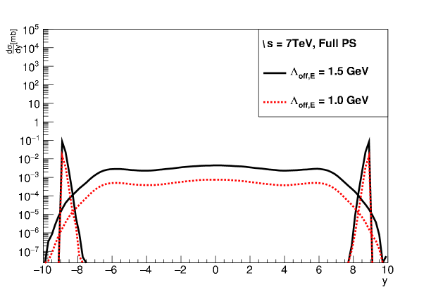
Figure 4: Rapidity distribution of protons (external peaks) and pions (internal bumps) for the full phase space for two different values of $\Lambda_{off,E}$ = 1, 1.5 GeV.

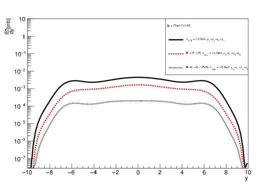
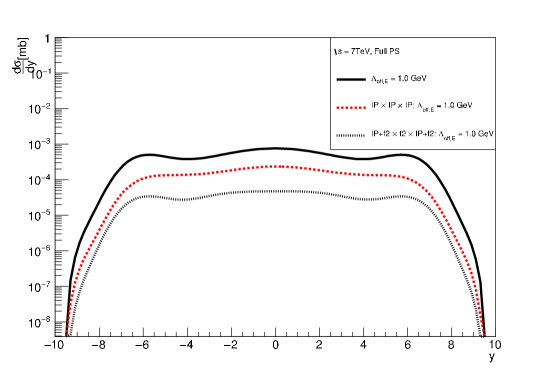
Figure 5: Rapidity distribution of pions for $(\mathbb{P}+f_{2\mathbb{R}})\times(\mathbb{P}+f_{2\mathbb{R}})\times(\mathbb{P}+f_{2\mathbb{R}})$ (upper curve), $\mathbb{P}\times\mathbb{P}\times\mathbb{P}$ (middle curve) and $(\mathbb{P}+f_{2\mathbb{R}})\times f_{2\mathbb{R}}\times(\mathbb{P}+f_{2\mathbb{R}})$ (lower curve) exchanges for two different values of $\Lambda_{off,E}$ = 1, 1.5 GeV.

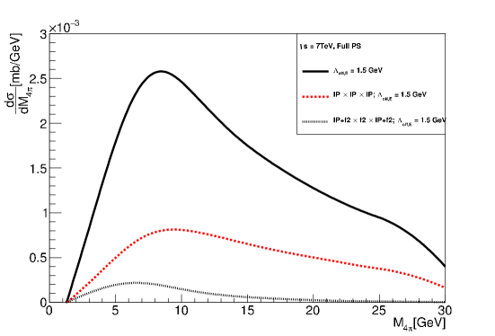
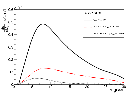
Figure 6: $4\pi$ invariant mass distribution for $(\mathbb{P}+f_{2\mathbb{R}})\times(\mathbb{P}+f_{2\mathbb{R}})\times(\mathbb{P}+f_{2\mathbb{R}})$ (upper curve), $\mathbb{P}\times\mathbb{P}\times\mathbb{P}$ (middle curve) and $(\mathbb{P}+f_{2\mathbb{R}})\times f_{2\mathbb{R}}\times(\mathbb{P}+f_{2\mathbb{R}})$ (lower curve) exchanges for two different values of $\Lambda_{off,E}$ = 1, 1.5 GeV.

In Fig. 7 we discuss distribution in dipion invariant mass separately for the opposite-sign pions (left panel) and for the same-sign pions (right panel). To improve statistics and reduce fluctuations the distributions for different combinations of indices (34, 56, 36, 45 for the opposite-sign pions or 35, 46 for the same-sign pions) were averaged in all figures of this type. The distributions for the opposite-sign pions have a large component at low ($M_{\pi\pi}<3$ GeV) dipion invariant mass, similarly to the dipion mass distribution for the exclusive dipion production (see e.g. LNS2016_2pi ). The distribution for the same-sign pions is clearly broader than that for the opposite-sign pions and has maximum at larger invariant masses. This is due to the possible presence of the rapidity gap between the two $\pi^{+}\pi^{-}$ pairs, as illustrated in Figs. 23 and 24, where we plot the differential cross section for the $(+-)(+-)+(-+)(-+)$, $(+-)(-+)+(-+)(-+)$ and $(++)(--)+(--)(++)$ configurations of ordered in rapidity pions as a function of the central rapidity gap width. It is clear that the same sign pion pairs are often formed across the large rapidity gap, what is reflected by the width of their invariant mass distribution Fig. 7. This is also related to the somewhat arbitrary cut-off approach to the region where the Regge formalism (10) does not apply. The higher invariant dipion masses are only weakly dependent on the cut-off of the low masses of the two pions across the pomeron/reggeon exchange. It is not clear to us how to correctly include this region.

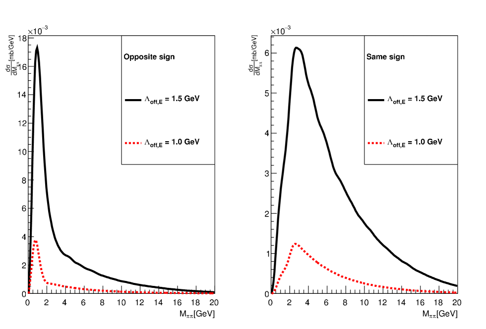
Figure 7: Dipion invariant mass distributions for the opposite-sign (left panel) and for the same-sign (right panel) pions for two different values of $\Lambda_{off,E}$ = 1 GeV (lower curve) and $\Lambda_{off,E}$ = 1.5 GeV (upper curve).

The shapes of the distributions in dipion invariant masses only slightly depend on the value of the cut-off parameter of the off-shell form factor (19). The position of the maximum for the same-sign pions at $M_{\pi\pi}\sim$ 3 GeV seems to be related to the point in $M_{\pi\pi}$ where we gradually screen off the Regge amplitude (see Eq. (10)). The position of the transition from the Regge to non-Regge physics have been taken here (somewhat arbitrarily) to be 3 GeV. Therefore our predictions are valid above $M_{\pi\pi}>$ 3 GeV. What happens below $M_{\pi\pi}$ = 3 GeV is rather a matter of future measurements. Clearly our approach is not valid in this region and therefore has no predictive power there.

For illustration in Fig. 8 we show dependence of the integrated cross section on the sharp cut-off parameter $W_{cut}$ (see Eq. (21)). One can observe a power-like dependence of the cross section as a function of $W_{cut}$. The extra crosses in the figure show the value of $W_{0}$ and the corresponding cross section in the smooth cut-off approach (see Eq. (20)). Such a value of $W_{0}$ was used in the description of the $pp\to pp\pi^{+}\pi^{-}$ process (see LS_2pi ).

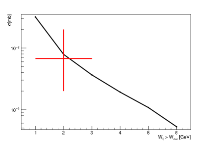
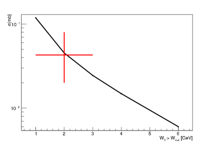
Figure 8: Integrated cross section for different values of $W_{cut}$ for sharp (Heaviside-like) cut-off function. The extra (red on line) cross represents cross section for the smooth cut-off function with $W_{0}$ = 2 GeV and $a$ = 0.2 GeV as taken from LS_2pi . The left figure is for $\Lambda_{off,E}=1$ GeV and the right one for $\Lambda_{off,E}=1.5$ GeV.

As it is seen the cross section for $W_{0}$ = 2 GeV (smooth cut-off) is very much the same as the cross section for $W_{cut}\sim 2-2.5$ GeV (sharp cut-off).

Finally, in Fig. 9 we show how the choice of $W_{cut}$ (sharp cut-off) influences the distributions. As an example we consider dipion mass spectra, where the effect of cut-off function is the most visible. In this calculation we fixed $\Lambda_{off,E}$ = 1.5 GeV and we show results for three different values of $W_{cut}$. The sharp cut-off leads to characteristic sudden increase of the cross section. The large part of the dipion distributions is only weakly dependent on the value of $W_{cut}$, but some visible effect survive (see the location of the dips in Fig. 9). This means that the different dipion subsystems are to some extend correlated. The study performed here was only to illustrate the possible uncertainties of our predictions. However, we believe that our default smooth cut-off is the optimal choice at present. We feel one should return to the problem when corresponding experimental data will be available.

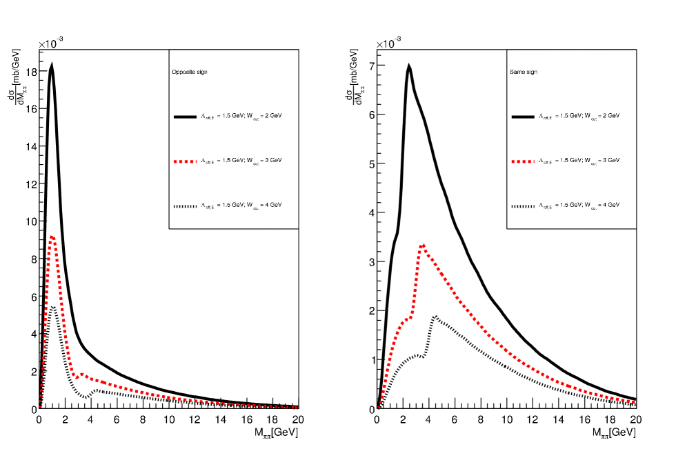
Figure 9: Dipion invariant mass distributions for the opposite-sign (left panel) and the same-sign (right panel) pions for different values of $W_{cut}$ for sharp cut-off function (21) and $\Lambda_{off,E}=1.5$ GeV.

III.2 Results for ATLAS cuts

In this subsection we present results relevant for the ATLAS experimental cuts. The following kinematical conditions are imposed:

$$|t_{1}|,|t_{2}|<1\;{\rm GeV}^{2}\,,\quad|y_{\pi}|<2.5\,,\quad p_{t,\pi}>0.5\;{\rm GeV}\,.$$ (23)

In addition, the mentioned above technical cut $M_{4\pi}<30$ GeV is imposed.

The corresponding integrated cross sections for different values of the cut-off parameter are collected in Tab. 2. In this case the dependence on $\Lambda_{off,E}$ is even stronger than for the full phase space case. This means that precise prediction of the cross section is not simple.

Table 2: Integrated cross sections in nb with the ATLAS cuts (23) for different values of the cut-off parameter $\Lambda_{off,E}$. No absorption effects are included here.

	$\Lambda_{off,E}$ [GeV]	$\sigma$ [nb]
ATLAS	1.0	6.91
ATLAS	1.5	141.43

Similarly as for the full phase space case we present several differential distributions in Figs. 10, 11, 12, 13.

The transverse momentum distribution of the four-pion system is shown in Fig. 10. The shape of the distribution is practically the same as for the full phase space case.

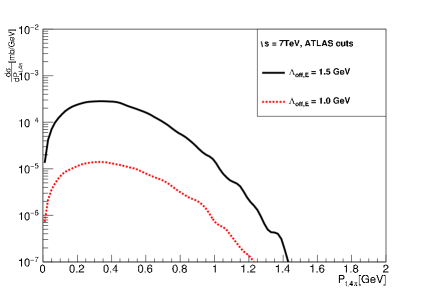
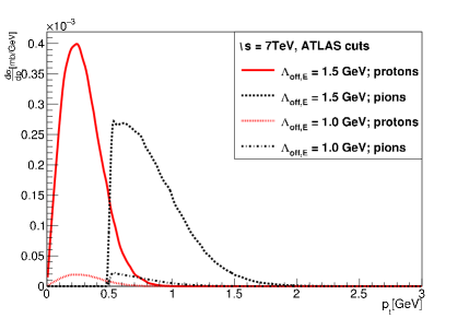
Figure 10: Distribution in transverse momentum of the four-pion system ($P_{t}$) (left panel) and for the transverse momenta of individual particles (protons or pions) (right panel) with the ATLAS cuts (23).

It should be noted that the distribution of the longitudinal momentum of the four-pion system after rapidity cuts related to the ATLAS central tracker acceptance (right side of Fig. 21) is very narrow in comparison to full phase space histogram shown in the same figure on the left side. The four-pion invariant mass distribution extends from $M_{4\pi}\approx 3$ GeV to the upper cut at $M_{4\pi}=30$ GeV. This means that the ATLAS experiment has a potential to investigate the discussed here mechanism.

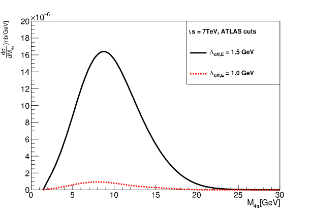
Figure 11: Four-pion invariant mass distribution ($M_{4\pi}$) with the ATLAS cuts (23) for $\Lambda_{off,E}=1$ GeV (lower curve) and $\Lambda_{off,E}=1.5$ GeV (upper curve).

The rapidity distributions of pions (middle bump) and protons (external peaks) are shown in Fig. 12. Here the rapidity coverage of the main tracker is clearly visible. The rapidity gaps between protons with $y\approx\pm$ 9 and pions are now set by the experimental cuts and are bigger than 4.5 rapidity units. But we have to assure, in addition, the existence of rapidity gap within the four-pion system confined now to $|y_{\pi}|<2.5$. Then the maximal rapidity gap is clearly confined from above to only five rapidity units.

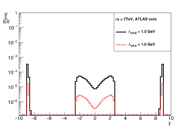
Figure 12: Distribution in rapidity of pions and protons for the ATLAS cuts (23).

In Fig. 13 we show dipion invariant mass distribution for the opposite-sign (left panel) and the same-sign (right panel) pions for two different values of $\Lambda_{off,E}$.

One major weakness of the discussed model is a rather simplistic treatment of the low dipion and $\pi p$ invariant masses i.e. non-Regge region. These region can be removed from the data imposing additional cut $M_{ij}>M_{ij,cut}\approx$ 2 – 4 GeV.

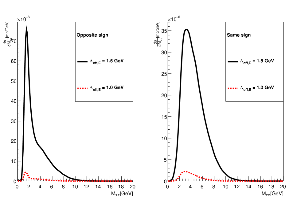
Figure 13: Dipion invariant mass distribution for the opposite-sign (left panel) and same-sign (right panel) pions with the ATLAS cuts (23) for different values of $\Lambda_{off,E}$.

Imposing such cuts leads to the cross sections collected in Tab. 3. The rate of the reduction of cross section depends on the value of the cut-off parameter and the way how amplitudes are modified in the difficult to control non-Regge region.

Table 3: The integrated cross sections in nb for the ATLAS cuts (23) with the extra limitations on $\pi\pi$ and $p\pi$ invariant masses. The columns ’Smooth’ show the resulting cross sections for the cut-off function of (20). The columns ’Sharp’ show results obtained for the cut-off function of (21) with $W_{cut}$ = 2 GeV. No absorption effects are included here.

	$\Lambda_{off,E}$ = 1.0 GeV		$\Lambda_{off,E}$ = 1.5 GeV
	Smooth	Sharp	Smooth	Sharp
no extra cut on $M_{ij}$	7.35	6.91	148.83	141.43
$M_{ij,cut}=2$ GeV	7.35	6.90	146.92	141.33
$M_{ij,cut}=3$ GeV	6.66	6.31	138.79	134.10
$M_{ij,cut}=4$ GeV	5.15	4.82	116.54	113.73

These experimental cuts remove influence of the details of the cut-off function on $M_{\pi\pi}$ plots, see Fig. 14.

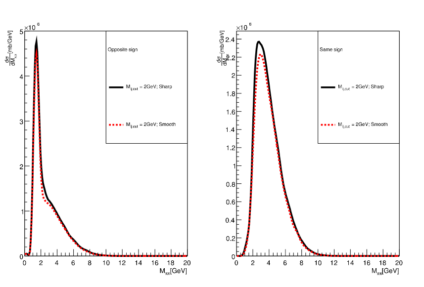
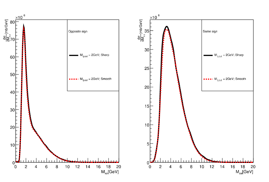
Figure 14: Dipion invariant mass distributions for the opposite-sign (left panel) and the same-sign (right panel) pions for the ATLAS experimental cuts (23) with the extra limitations on $M_{ij}>M_{ij,cut}$. The upper plot is for $\Lambda_{off,E}=1$ GeV and the lower one for $\Lambda_{off,E}=1.5$ GeV. ’Smooth’ means cut-off (20) with $W_{0}=2$ GeV and ’Sharp’ means cut-off (21) with $W_{cut}=2$ GeV.

These additional cuts ($M_{ij.cut}=2$ GeV) practically do not change the distributions shown in Fig. 13. The same can be seen by comparison of first two rows of Tab. 3.

III.3 Results for ALICE cuts

For the ALICE experiment we take the following cuts:

$$p_{t,p}<2\;{\rm GeV}\,,\quad p_{t,\pi}>0.17\;{\rm GeV}\,,\quad|\eta_{\pi}|<0.9\,,$$ (24)

and the technical $M_{4\pi}<30$ GeV cut. Corresponding numerical values for the integrated cross sections are presented in Tab. 4. They are rather small compared to the ATLAS case.

Table 4: Integrated cross sections in pb for the ALICE cuts (24) for the smooth cut-off function and for different values of $\Lambda_{off,E}$. No absorption effects are included here.

	$\Lambda_{off,E}$ [GeV]	$\sigma$ [pb]
ALICE	1.0	$\;\,4.2$
ALICE	1.5	$37.7$

Several differential distributions are presented below in Figs. 16, 17 and 18. The distribution in transverse momentum of the four-pion system (Fig. 15) is here very similar as those for the full phase space and for the ATLAS cuts. In contrast, the distribution in four-pion invariant mass drops faster than its counterpart for the ATLAS case. The irregular structures are due to narrow rapidity coverage of the ALICE detector and/or the cuts on each exchange of the pomeron or reggeon. The cross section for the triple Regge mechanism is for the ALICE fiducial volume very small, see Tab. 4. In addition, other mechanisms (see LNS2016_4pi ) may be important in this region. We conclude that the ALICE detector is not well suited for the studies of processes with three pomeron/reggeon exchanges.

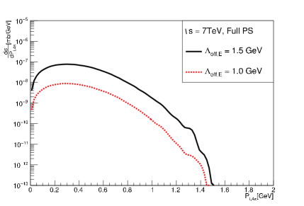
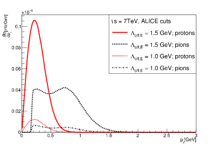
Figure 15: Distribution in transverse momentum of the $4\pi$ system (left panel) and in transverse momenta of individual pions or protons (right panel) for the ALICE cuts (24) and for the two values of $\Lambda_{off,E}$ specified in the figure legends.

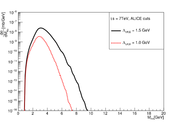
Figure 16: Four-pion invariant mass distribution for the ALICE cuts (24) and for $\Lambda_{off,E}=1$ GeV (lower curve) and $\Lambda_{off,E}=1.5$ GeV (upper curve).

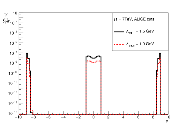
Figure 17: Distribution in rapidity of pions (middle bump) and of protons (external peaks) for the ALICE cuts for two different values of $\Lambda_{off,E}$.

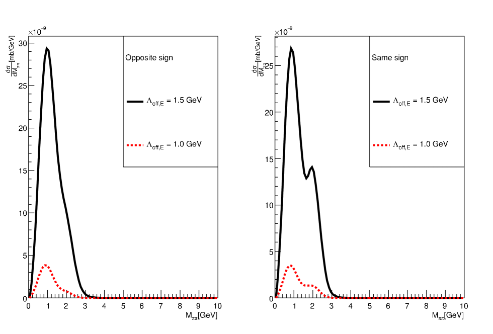
Figure 18: Dipion invariant mass distribution for the opposite sign (left panel) and the same sign (right panel) pions for the ALICE cuts (24).

IV Discussion of some additional aspects of the triple-Regge exchange model

Here we discuss in more detail some aspects of the model only mentioned in the previous section.

IV.1 $M_{4\pi}$ distribution and energy transfer to the $4\pi$ system

Here we wish to discuss some kinematic properties of the $4\pi$ system. In particular, we wish to understand how much energy can be transferred to the four-pion system. In our opinion, this is determined by the fact that the scattered protons take almost all energy leaving only a small amount of available energy which is distributed among the all centrally produced final pions. This can be traced back to specific propagators of pomerons/reggeons that couple to protons. In this subsection we shall try to justify the hypothetical statement.

In order to better understand this effect we first plot distribution in energy of one of outgoing protons in Fig. 19. The distribution quickly drops towards energies smaller than $\sqrt{s}/2$ which in our example is 3.5 TeV. For the case of the ATLAS cuts (23) the drop is much faster.

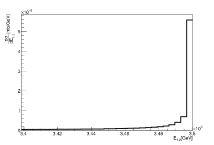
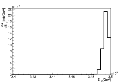
Figure 19: Proton energy distributions for the full phase space (left) and for the ATLAS cuts (23) (right). Here we take $\Lambda_{off,E}=1.5$ GeV as an example.

Summing energies of both outgoing protons we obtain total energy taken by protons. In Fig. 20 we show distribution in the energy left for pions, which is the total energy minus the energy taken away by protons. The energies left for pions are much smaller than those taken away by protons. Kinematics dictates the following inequality:

$$M_{4\pi}<\sqrt{s}-E_{1}-E_{2}\,.$$ (25)

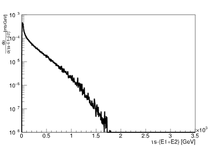
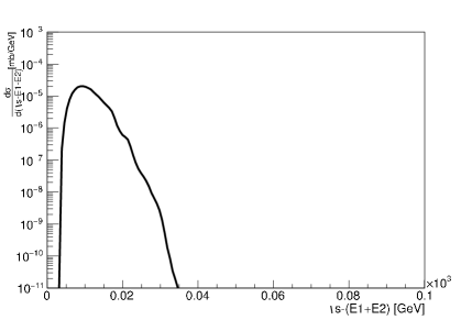
Figure 20: Distributions in the energy left for pions for the full phase space (left) and for the ATLAS cuts (23) (right). Here we take $\Lambda_{off,E}=1.5$ GeV. For the full phase space case there is visible a sharp break above $1500$ GeV indicating numerical accuracy limit.

For our process the dynamics imposes much severe cuts so it means the restriction (25) is not really important.

In general, the whole four-pion system does not need to be at rest in the overall centre of mass system. Let us define the quantity:

$$P_{4\pi,z}=p_{3,z}+p_{4,z}+p_{5,z}+p_{6,z}\;.$$ (26)

In Fig. 21 we show distribution of the $P_{4\pi,z}$ variable. We observe much narrower distribution in the case of the ATLAS fiducial volume compared to the full phase space case. In the case of full phase space (left panel) the four-pion system is created with relatively large longitudinal momenta. For the ATLAS cuts (right panel) the four-pion system is almost at rest and the whole available energy is transferred to the excitation of the four-pion system.

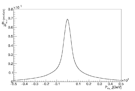
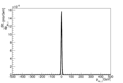
Figure 21: Distributions in the longitudinal momentum of the pion center of mass for the full phase space (left) and for the ATLAS cuts (23) (right). Here we take $\Lambda_{off,E}=1.5$ GeV as an example.

IV.2 Interference effect

In this subsection we investigate interference between graphs in the whole amplitude. In order to quantify this effect we propose to compare the cross section for the full amplitude of (2), with the cross section obtained by adding matrix element squared of individual diagrams, i.e.,

$$\begin{split}|{\cal M}_{\textrm{no interference}}|^{2}&=\frac{1}{4}\left(|{\cal M}_{\{3456\}}|^{2}+|{\cal M}_{\{5436\}}|^{2}+|{\cal M}_{\{3654\}}|^{2}+|{\cal M}_{\{5634\}}|^{2}\right)+\ldots.\\ \end{split}$$ (27)

The plots for the full phase space are presented in Fig. 22.

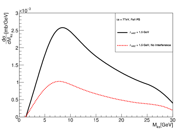
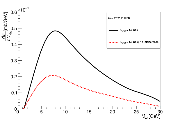
Figure 22: Four-pion invariant mass distribution for the full phase space for two different values of $\Lambda_{off,E}$.

The amount of the interference can be considered as a measure of rapidity ordering characteristic for high energy multiperipheral processes. For fully ordered events i.e. with large rapidity gaps between all particles the interference effect is small because identical particles occupy different regions of phase space and the amplitude with reversed order is damped by the factor responsible for peripherality of the process. In our case the identical pions are often spaced by the large rapidity gap (see Figs.23 and 24), however, low rapidity gap spacing component is also strong. As result interference effect contributes to $\sim 1/2$ of the cross section as seen in Fig. 22.

IV.3 Rapidity ordering of pions and the gap between two pion systems

In this subsection the rapidity gap between different orderings in rapidity of pions will be presented. This variable can well distinguish different central particles, however, any other variable that separates pions can be used. The procedure can be used in experiment to characterize triple pomeron/reggeon exchange process. The idea is as follows. The pions will be ordered with respect to their rapidities. Assume that the rapidities of pions are ordered in the following way $y_{1}<y_{2}<y_{3}<y_{4}$. The distribution in rapidity difference between pions $2$ and $3$ will be presented. Three different classes of the ordering of pion charges are possible in general. The class $A$:

• $\pi^{+}(y_{1})$, $\pi^{-}(y_{2})$, $\pi^{+}(y_{3})$, $\pi^{-}(y_{4})$,

• $\pi^{-}(y_{1})$, $\pi^{+}(y_{2})$, $\pi^{-}(y_{3})$, $\pi^{+}(y_{4})$,

the class $B$:

• $\pi^{-}(y_{1})$, $\pi^{+}(y_{2})$, $\pi^{+}(y_{3})$, $\pi^{-}(y_{4})$,

• $\pi^{+}(y_{1})$, $\pi^{-}(y_{2})$, $\pi^{-}(y_{3})$, $\pi^{+}(y_{4})$,

and the class $C$:

• $\pi^{+}(y_{1})$, $\pi^{+}(y_{2})$, $\pi^{-}(y_{3})$, $\pi^{-}(y_{4})$,

• $\pi^{-}(y_{1})$, $\pi^{-}(y_{2})$, $\pi^{+}(y_{3})$, $\pi^{+}(y_{4})$.

In Figs. 23 and 24 we present distributions in rapidity difference between the second and the third pion for full phase space and for the ATLAS kinematical cuts (23). These plots show the characteristics of the triple-Regge process which can be verified experimentally.

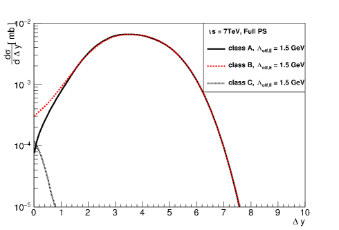
Figure 23: Rapidity difference between second and the third pion for $\Lambda_{off,E}=1.5$ GeV for full phase space.

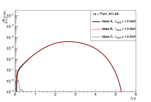
Figure 24: Rapidity difference between second and the third pion for $\Lambda_{off,E}=1.5$ GeV for the ATLAS detector cuts.

As can be seen from the figures, the events for the class $C$ happens much more rarely than the events for classes $A$ or $B$. In addition, the gap for the class $C$ is much smaller than for classes $A$ and $B$. This is because pion exchange is responsible for the gap for the class $C$ versus pomeron exchange for classes $A$ and $B$.

IV.4 Comparison with $2\sigma$ production

The $pp\rightarrow pp\sigma\sigma$ process recently discussed in LNS2016_4pi , due to the decay $\sigma\rightarrow\pi^{+}\pi^{-}$, produces the same final state as the triple-Regge $pp\rightarrow pp4\pi$ process.

The Born-level results for the continuum mechanism including ATLAS cuts (23) for $\sqrt{s}=7$ and 13 TeV, see Tab. 5, should be compared to 750.56 nb and 847.46 nb, respectively, from the sequential $pp\to pp(\sigma\sigma\to 4\pi)$ process discussed in LNS2016_4pi (please note that a slightly different cuts were used there). Note that these values of cross section are smaller than in Table I of LNS2016_4pi where $p_{t,\pi}>0.1$ GeV was imposed in the calculations. The cross sections for the $\sigma\sigma$ mechanism was obtained with the coupling constants given by (2.12) of LNS2016_4pi and the off-shell $t$-channel $\sigma$ meson form factor (2.13) of LNS2016_4pi with $\Lambda_{off,E}=1.6$ GeV.

These two mechanisms are complementary as can be seen in Fig. 25, as they occupy different range of $M_{4\pi}$. In addition, in the range $2{\rm~{}GeV}<M_{4\pi}<4{\rm~{}GeV}$ the $\sigma\sigma$ mechanism dominates with a rather sharp peak at $M_{4\pi}\sim 3$ GeV and the triple-Regge contribution dominates above $8$ GeV. These characteristics could be very useful when trying experimental distinctions of these two processes.

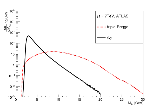
Figure 25: Four-pion invariant mass distribution ($M_{4\pi}$) with the ATLAS kinematical cuts (23) for $\sqrt{s}=7$ TeV. The results correspond to the Born level calculations. The dotted line represents the triple Regge exchange mechanism obtained for $\Lambda_{off,E}=1.5$ GeV. The solid line represents the contribution from $\sigma\sigma$ mechanism discussed in LNS2016_4pi .

IV.5 Predictions for LHC at $13$ TeV

In this subsection we wish to provide also first predictions for current runs at the LHC at $\sqrt{s}=13$ TeV. A more detailed analysis, including technical details of experiments, will be postponed to a separate paper.

In Tab. 5 numerical values of the cross section are given and compared to out previous results.

Table 5: The integrated Born level (no absorption effects) cross section for the four-pion continuum production. Results were calculated for two different values of the cut-off parameter $\Lambda_{off,E}$ (19).

	$\Lambda_{off,E}$ [GeV]	$\sigma$ $@$ $\sqrt{s}=7$ TeV	$\sigma$ $@$ $\sqrt{s}=13$ TeV
Full PS	1.0	7.21 $\mu$b	8.97 $\mu$b
Full PS	1.5	42.86 $\mu$b	51.78 $\mu$b
ATLAS	1.0	6.91 nb	7.48 nb
ATLAS	1.5	141.43 nb	154.19 nb
ALICE	1.0	4.2 pb	4.7 pb
ALICE	1.5	37.7 pb	42 pb

The table shows that the transfer of energy to the system is slowly varying with the collision energy. Therefore all plots presented in the previous sections do not differ dramatically for the case of $\sqrt{s}=13$ TeV. The only sizeable difference is that in the rapidity plots the protons are a bit further from $y=0$. Summing up, the model cross section is only weakly dependent on the centre-of-mass energy.

V Conclusions

The triple-Regge exchange model was proposed for the production of four-pions in the $pp\to pp\pi^{+}\pi^{-}\pi^{+}\pi^{-}$ exclusive reaction. The amplitudes of the process were parametrized in the Regge formalism with coupling constants fixed to describe the total nucleon-nucleon and pion-nucleon cross sections. Some care must be taken how to ’remove’ the low dipion invariant mass regions ($M_{\pi\pi}<2$ GeV) that are not described by Regge amplitudes

In the considered process two of the pions are off-mass-shell already in the Born amplitude(s). The off-shell effects are parametrized in terms of corresponding form factors. The same objects (form factors) were discussed recently in the context of the $pp\to pp\pi^{+}\pi^{-}$ reaction considered both theoretically as well as measured by the STAR, CDF, and CMS collaborations STAR ; CDF ; CMS . The cut-off parameter was fitted then LNS2016_2pi to describe the preliminary data. The present dipion data do not allow for a precise extraction of the model parameter but allow to obtain a reasonable range of the cut-off parameter $\Lambda_{off,E}$ = 1 – 1.5 GeV. Here we have assumed exponential dependence of the form factors on the pion virtualities. Then the model has almost only one free parameter (called here cut-off parameter), which can be taken in the range known from the four-body ($pp\to pp\pi^{+}\pi^{-}$) reaction studied in the literature. In comparison to the four-body reaction the dependence on the cut-off parameter is much stronger as two pions, instead of one for the $pp\rightarrow pp\pi^{+}\pi^{-}$ process, are off-mass-shell.

We have made first predictions for the six-body processes. Both total cross sections (integrated over six-body phase space) as well as several differential distributions were calculated and presented. Compared to the $\sigma\sigma$ and $\rho\rho$ mechanisms considered recently by two of us LNS2016_4pi , the considered here mechanism populates final states with much larger dipion and four-pion invariant masses. We get total cross section 7.21 – 42.86 $\mu$b (see Tab. 5) in the whole phases space (neglecting absorption effects!). The absorption effects are expected to diminish the cross section by an order of magnitude. Our preliminary studies here have been done at the Born level and the absorption can be included only in the form of the multiplicative gap survival factor. One expects it to be of the order of 0.1. Full-fledged calculation of absorption effects and in particular its dependence on kinematical variables is not simple (see, e.g., LS2015 for detailed studies for the $pp\to pp\pi^{+}\pi^{-}$ reaction).

The integrated full phase space cross section cannot be, however, measured due to limited coverage of the LHC detectors. We have therefore made predictions for the kinematical cuts characteristic for the ATLAS and ALICE detectors. The latter detector can identify pions down to very small transverse momenta of $p_{t,\pi}$ = 0.1 GeV. However, the rapidity coverage of the ALICE tracker is very (too) limited. This does not allow to observe the large four-pion invariant masses, the genuine feature of the considered diffractive triple-Regge mechanism. In contrast, the ATLAS detector allows to measure cases with large $4\pi$ invariant masses. We expect that the considered multi-diffractive process dominates over the contributions of other mechanisms for four-pion invariant masses $M_{4\pi}>10$ GeV.

We have discussed in addition how much energy can be transferred from protons to the excitation of the four-pion system. We have demonstrated that the model amplitude gives natural limitations for such a transfer. A specific ordering of pion charges in rapidity has been found to be an interesting and representative characteristics of the discussed process.

To assure exclusivity of the process, not only charged pions but also forward/backward protons should be measured. The ALFA detectors are natural candidates for this purpose in the case of the ATLAS experiments. Similarly the CMS collaboration together with the TOTEM collaboration could perform similar studies.

In summary, the observation of counts/events at large four-pion invariant masses should be a clear signal of observing the discussed here three-pomeron exchange processes, not identified so far experimentally.

Appendix A Peripheral reaction with decay of central system

In this section (appendix) we presents the recipe for generating phase space of the reaction which treats all final pions in the same way and therefore it is suitable for the case when including complicated interferences of contributing amplitudes. The considered reaction is of the form: $p(p_{a})+p(p_{b})\rightarrow p(p_{1})+p(p_{2})+CM(P_{4\pi})$ and then $CM(P_{4\pi})\rightarrow\pi^{+}(p_{3})+\pi^{-}(p_{4})+\pi^{+}(p_{5})+\pi^{-}(p_{6})$. The formula for the cross section can be written in the standard form

$$\sigma=\int(2\pi)^{4}\frac{\overline{|{\cal M}|^{2}}}{2s}\delta^{(4)}\left(P-\sum_{i=1}^{6}p_{i}\right)\prod_{i=1}^{6}\frac{d^{3}p_{i}}{(2\pi)^{3}2E_{i}}\,,$$ (28)

where ${\cal M}$ is a matrix element for the six-body reaction and $P=p_{a}+p_{b}$ is a total four-momentum in the initial (and final) system.

Starting from (28) the phase space is factorized as (see Pilkuhn , Eq. (9.7))

$$\begin{split}&\sigma=\int_{4m_{\pi}}^{\infty}dM_{4\pi}^{2}\int(2\pi)^{4}\delta^{(4)}\left(P-p_{1}-p_{2}-P_{4\pi}\right)\frac{d^{3}p_{1}}{(2\pi)^{3}2E_{1}}\frac{d^{3}p_{2}}{(2\pi)^{3}2E_{2}}\frac{d^{3}P_{4\pi}}{(2\pi)^{3}2E_{4\pi}}\\ &\qquad\times\frac{1}{2\pi}\int(2\pi)^{4}\delta^{(4)}(P_{4\pi}-\sum_{i=3}^{6}p_{i})\prod_{i=3}^{6}\frac{d^{3}p_{i}}{(2\pi)^{3}2E_{i}}\frac{\overline{|{\cal M}|^{2}}}{2s}\,,\end{split}$$ (29)

where the integration over $M_{4\pi}$ variable extends from the threshold for the $4\pi$ production to the infinity (in our case to the technical cut $M_{4\pi}<30$ GeV). The second decay of the central system $P_{4\pi}$ into four particles can be calculated using slightly modified sequence of decays of the GENBOD CERN library (currently the TGenPhaseSpace class from ROOT package ROOT_site ). For a description of the algorithm of the generation see JamesCERN . This modification will be described elsewhere.

This prescription is the best choice for matrix elements with permutation of identical particles, as it treats all centrally produced particles on the same footing.

In our practical realization the phase space available for the process is fairy large which requires special technical treatment event for adaptive Monte Carlo generator. The most efficient solution is to divide the whole range of $M_{4\pi}$ into smaller exclusive intervals and add distributions for the different intervals.

References

- (1) P. Lebiedowicz and A. Szczurek, Phys. Rev. D81 (2010) 036003.
- (2) P. Lebiedowicz and A. Szczurek, Phys. Rev. D83 (2011) 076002.
- (3) P. Lebiedowicz and A. Szczurek, Phys. Rev. D85 (2011) 014026.
- (4) R. A. Kycia, J. Chwastowski, R. Staszewski, and J. Turnau, arXiv:hep-ph/1411.6035.
- (5) P. Lebiedowicz, O. Nachtmann, and A. Szczurek, Phys. Rev. D93 (2016) 054015.
- (6) P. Lebiedowicz, O. Nachtmann, and A. Szczurek, Phys. Rev. D94 (2016) 034017.
- (7) A. Breakstone et al. (ABCDHW Colaboration), Z. Phys. C58 (1993) 251.
- (8) A. Donnachie, H. G. Dosch, P. V. Landshoff, and O. Nachtmann, “Pomeron physics and QCD”, Camb. Monogr. Part. Phys. Nucl. Phys. Cosmol. 19 (2002) 1.
- (9) R. Staszewski, P. Lebiedowicz, M. Trzebinski, J. Chwastowski, and A. Szczurek, Acta Phys. Polon. B42 (2011) 1861.
- (10) P. Lebiedowicz and A. Szczurek, Phys. Rev. D92 (2015) 054001.
- (11) H. Pilkuhn, “The Interactions of Hadrons”, North-Holland Publishing Company, 1967.
- (12) ROOT software, http://root.cern.ch/drupal/
- (13) F. James, CERN 68-15 (1968).
- (14) L. Adamczyk, W. Guryn, and J. Turnau, Int. J. Mod. Phys. A29 (2014) 28, 1446010.
- (15) T. A. Aaltonen et al. (CDF Collaboration), Phys. Rev. D91 (2015) 091101.
- (16) (CMS Collaboration), Report No. CMS-PAS-FSQ-12-004.