Distributed Representation of Subgraphs

Abstract.

Network embeddings have become very popular in learning effective feature representations of networks. Motivated by the recent successes of embeddings in natural language processing, researchers have tried to find network embeddings in order to exploit machine learning algorithms for mining tasks like node classification and edge prediction. However, most of the work focuses on finding distributed representations of nodes, which are inherently ill-suited to tasks such as community detection which are intuitively dependent on subgraphs.

Here, we propose Sub2Vec, an unsupervised scalable algorithm to learn feature representations of arbitrary subgraphs. We provide means to characterize similarties between subgraphs and provide theoretical analysis of Sub2Vec and demonstrate that it preserves the so-called local proximity. We also highlight the usability of Sub2Vec by leveraging it for network mining tasks, like community detection. We show that Sub2Vec gets significant gains over state-of-the-art methods and node-embedding methods. In particular, Sub2Vec offers an approach to generate a richer vocabulary of features of subgraphs to support representation and reasoning.

1. Introduction

Graphs are a natural abstraction for representing relational data from multiple domains such as social networks, protein-protein interactions networks, the World Wide Web, and so on. Analysis of such networks include classification (Bhagat et al., 2011), link prediction (Liben-Nowell and Kleinberg, 2007), detecting communities (Girvan and Newman, 2002; Blondel et al., 2008), and so on. Many of these tasks can be solved using machine learning algorithms. Unfortunately, since most machine learning algorithms require data to be represented as features, applying them to graphs is challenging due to their high dimensionality and structure. In this context, learning meaningful feature representation of graphs can help to leverage existing machine learning algorithms more widely on graph data.

Apart from classical dimensionality reduction techniques (see related work), recent works (Perozzi et al., 2014; Grover and Leskovec, 2016; Wang et al., 2016; Tang et al., 2015) have explored various ways of learning feature representation of nodes in networks exploiting relationships to vector representations in NLP (like word2vec (Mikolov et al., 2013)). However, application of such methods are limited to binary and muti-class node classification and edge-prediction. It is not clear how one can exploit these methods for other tasks like community detection which are inherently based on subgraphs and node embeddings result in loss of information of the subgraph structure. Embedding of subgraphs or neighborhoods themselves seem to be better suited for these tasks. Surprisingly, learning feature representation of networks themselves (subgraphs and graphs) has not gained much attention thus far. In this paper, we address this gap by studying the problem of learning distributed representation of subgraphs. Our contributions are:

1. We propose Sub2Vec, a scalable subgraph embedding method to learn features for arbitrary subgraphs that maintains the so-called local proximity.

2. We also provide theoretical justification of network embedding using Sub2Vec, based on language modeling tools. We also propose meaningful ways to measure how similar two subgraphs are to each other.

3. We conduct multiple experiments over large diverse real datasets to show correctness, scalability, and utility of features learnt by Sub2Vec in several tasks. In particular we get upto 4x better results in tasks such as community detection compared to just node-embeddings.

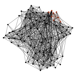
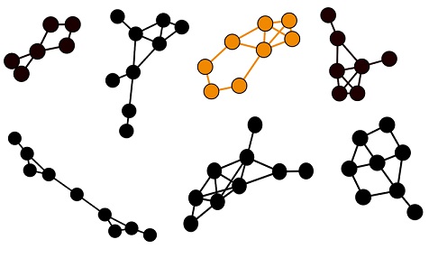
(a) A network $G$	(b) A set, $\mathcal{S}$, of subgraphs of $G$	(c) embedding learned for each subgraph	(d) Intermediate neighborhoods
			on each subgraph

Figure 1. An overview of our Sub2Vec. Our input is a set of subgraphs $\mathcal{S}$ drawn from a network $G$. We obtain $d$ dimensional embedding of subgraphs such that we maximize the likelihood of observing intermediate neighborhoods.

The rest of the paper is organized as follows: we first formulate and motivate our problem, then present Sub2Vec, discuss experiments, and finally present related work, discussion and conclusions.

2. Problem Formulation

In this paper, we are interested in embedding subgraphs into a low dimensional continuous vector space. As shown later, the vector representation of subgraphs enables us to apply off-the-shelf machine learning algorithms directly to solve subgraph mining tasks. For example, to group subgraphs together, we can apply clustering algorithms like KMeans directly. Figure 1 (a-c) gives an illustration. Given a set of subgraphs (Figure 1 (b)) of a graph $G$ (Figure 1 (a)), we learn a low-dimensional feature representation of each subgraph (Figure 1(d)).

Now we are ready to formulate our Subgraph Embedding problem. We are given a graph $G(V,E)$ where $V$ is the vertex set, and $E$ is the associated edge-set (we assume undirected graphs here, but our framework can be easily extended to directed graphs as well). We define $g_{i}(v_{i},e_{i})$ as a subgraph of $G$, where $v_{i}\subseteq V$ and $e_{i}\subseteq E$. For simplicity, we write $g_{i}(v_{i},e_{i})$ as $g_{i}$. As input we require a set of subgraphs $\mathcal{S}=\{g_{1},g_{2},\dots,g_{n}\}$. Our goal is to embed subgraphs in $\mathcal{S}$ into $d$-dimensional feature space $\mathbb{R}^{d}$, where $d<<|V|$. In addition, we want to ensure the subgraph proximity is well-preserved in such a $d$-dimensional space. In this paper, we consider to preserve the “local neighborhood” of each subgraph $g_{i}$. The idea is that if two subgraphs share common structure, then their vector representations in $\mathbb{R}^{d}$ are close. We call such a measure Local Proximity.

Informal Definition 1.

(Local Proximity). Given two subgraphs $g_{i}(v_{i},e_{1})$ and $g_{j}(v_{j},e_{j})$, the local proximity between $g_{i}$ and $g_{j}$ is larger if the commonly induced subgraph is larger.

Intuitively, local proximity measures how many nodes, edges, and paths are shared by two subgraphs. For illustration of the local proximity, let us consider an example. In Figure 2, suppose $g_{1}$, $g_{2}$, and $g_{3}$ are subgraphs induced by nodes $\{a,b,c,e\}$ and $\{b,c,d,e\}$, and $\{d,e,f,j\}$. Since, the subgraph commonly induced by $g_{1}$ and $g_{2}$ is larger than the subgraph commonly induced by $g_{1}$ and $g_{3}$, we say $g_{1}$ and $g_{2}$ to be more “locally proximal” to each other than $g_{1}$ and $g_{3}$. Note that the local proximity is not just the Jaccard similarity of nodes in the two subgraphs, as it also takes the connections among the common nodes into account.

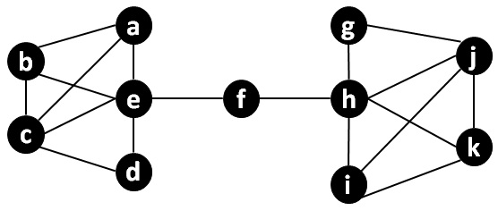
Figure 2. A toy network

Having defined the local proximity of two subgraphs, we focus on learning vector representations of subgraphs such that the local proximity is preserved. Formally, our Subgraph Embedding problem is,

Problem 1.

Given a graph $G(V,E)$, $d$ and set of $\mathcal{S}$ subgraphs (of $G$) $\mathcal{S}=\{g_{1},g_{2},\dots,g_{n}\}$, learn an embedding function $f:g_{i}\rightarrow\mathbf{y_{i}}\in\mathbb{R}^{d}$ such that Local Proximity among subgraphs is preserved.

According to Problem 1, if $g_{i}$ and $g_{j}$ are closer to each other in terms of the local proximity that $g_{k}$ and $g_{k}$ then the $\mathbf{sim}\left(f(g_{i}),f(g_{j})\right)$ has to be greater than $\mathbf{sim}\left(f(g_{i}),f(g_{k})\right)$, where $\mathbf{sim}(\mathbf{x},\mathbf{y})$ is a similarity metric between two real vectors $x$ and $y$ in $\mathbb{R}^{d}$. Hence, if we embed the subgraphs in Figure 2 from the previous example, then a correct algorithm to solve Problem 1 has to ensure that $\mathbf{sim}\left(f(g_{1}),f(g_{2})\right)>\mathbf{sim}\left(f(g_{i}),f(g_{j})\right)$. We propose an efficient algorithm for Problem 1 based on two different optimization objectives in the next section.

A natural question to ask is that if there are other metrics of subgraph similarity. Indeed, one can think of other measures of proximity, which may result in different embeddings. We will discuss this point further in Section 6.

3. Learning Feature Representations

In this section, we propose two optimization objectives for Problem 1 and propose an unsupervised deep learning technique to optimize the objectives.

Mikolov et al. proposed the continuous bag of words and skip-gram models in (Mikolov et al., 2013), which have been extensively used in learning continuous feature representation of words. Building on these two models, Le et al. (Le and Mikolov, 2014) proposed two models: the Distributed Memory of Paragraph Vector (PV-DM), and the Distributed Bag of Words version of Paragraph Vector (PV-DBOW), which can learn continuous feature representations of paragraphs and documents.

Our main idea is to pose our feature learning problem as a maximum likelihood problem by extending PV-DM and PV-DBOW to networks. The direct analog is to treat each node as a word, and each subgraph as a paragraph. The edges within a subgraph can be thought as the adjacency relation of two words in a paragraph. PV-DBOW and PV-DM assume that if two paragraphs share similar sequence of words, they are close in the embedded feature space. The local proximity of subgraphs naturally follows the above assumption. Hence, we can leverage deep learning techniques in (Le and Mikolov, 2014) for our subgraph embedding problem. PV-DBOW and PV-DM learn a latent representation by maximizing a distribution of word co-occurrences (using either n-gram or skip-gram model). Similarly, in this paper, we maximize a distribution of “node neighborhood”. The so-called “node neighborhood” is generated by subgraph-truncated random walks (see details in Section 3.3). We call our models Distributed Bag of Nodes version of Subgraph Vector (Sub2Vec-DBON) and Distributed Memory version of Subgraph Vector (Sub2Vec-DM) respectively.

Next, we will introduce Sub2Vec-DM, Sub2Vec-DBON first, then study how to generate “node neighborhood” and give a justification from matrix multiplication view. Finally, we summarize our algorithm Sub2Vec.

3.1. Sub2Vec-DM

In the Sub2Vec-DM model, we seek to predict a node $u$ given other nodes in $u$’s neighborhoods and the subgraph $u$ belongs to. Consider the subgraph $g_{1}$ (a subgraph induced by nodes $\{a,b,c,e\}$) in Figure 2. Suppose the sequence of nodes returned by random walks in $g_{1}$ is $[a,b,c]$, and we consider neighborhood of distance 2, then the model asks to predict node $c$ given subgraph $g_{1}$, and its predecessors ($a$ and $b$), i.e., $\Pr(c|g_{1},\{a,b\})$.

More precisely, given a $G^{\prime}(V^{\prime},E^{\prime})$ as the union graph of all the subgraphs in $\mathcal{S}=\{g_{1},g_{2},\dots,g_{n}\}$, where $V^{\prime}=\bigcup_{i}{v_{i}}$ and $E^{\prime}=\bigcup_{i}{e_{i}}$, consider a function $m$: $V^{\prime}\rightarrow\mathbb{R}^{d}$ ($m(n)=\mathbf{x}$). We define $\mathbf{M}$ as a $d\times|V^{\prime}|$ node vector matrix, where each column is $m(n)$ (the vector representation of nodes $n\in V^{\prime}$). Similarly, we define function $f(g_{i})$ as the embedding function for subgraph $g_{i}$, where $f(g_{i})$ is a $d$-dimensional vector. We denote $\mathbf{S}$ as the subgraph matrix, where each column is $f(g_{i})$ for all subgraphs in $\mathcal{S}$. The matrices $\mathbf{M}$ and $\mathbf{S}$ are indexed by node and subgraph ids. In Sub2Vec-DM, we use the node and subgraph vectors to predict the next node in the neighborhood $N_{n}$. We assume $N_{n}$ is given, and will discuss $N_{n}$ later in Section 3.3.

Now, given a node $n$ and its neighborhood $N_{n}$ and the subgraph $g_{i}$ from which the $N_{n}$ is drawn, the objective of Sub2Vec-DM is to maximize the following:

(1) $$\max_{f}\sum_{g_{i}\in\mathcal{S}}\sum_{n\in g_{i}}\log(\Pr(n|m(N_{n}),f(g_{i})),$$

where $\Pr(n|m(N_{n}),f(g_{i}))$ is the probability of predicting node $n$ in $g_{i}$ given the vector representations of its neighborhood $m(N_{n})$ and the subgraph from which the node and its neighborhood is drawn, $f(g_{i})$. Note that for ease of description, we extend the function $m$ from a node to a node set (neighborhood $N_{n}$). $\Pr(n|m(N_{n}),f(g_{i}))$ is defined using the softmax function:

(2) $$\Pr(n|m(N_{n}),f(g_{i}))=\frac{e^{\mathbf{U}_{n}\cdot h(m(N_{n}),f(g_{i}))}}{\sum_{v\in V}e^{\mathbf{U}_{v}\cdot h(m(N_{n}),f(g_{i}))}}$$

where matrix $\mathbf{U}$ is a softmax parameter and $h(\mathbf{x},\mathbf{y})$ is average or concatanation of vectors $\mathbf{x}$ and $\mathbf{y}$ (Le and Mikolov, 2014). In practice, to compute Equation 2, hierarchical softmax is used (Mikolov et al., 2013).

3.2. Sub2Vec-DBON

In the Sub2Vec-DBON model, we want to predict the nodes in the subgraph given only the subgraph vector $f(g_{i})$. For example, consider the same example in Section 3.1: the subgraph $g_{1}$ in Figure 2, and the node sequence $[a,b,c]$ generated by random walks. Now, in the Sub2Vec-DBON model the goal is to predict the neighborhood $\{a,b,c\}$ given the subgraph $g_{1}$. This model is parallel to the popular skip-gram model.

Formally, given a subgraph $g_{i}$, and neighborhood $N$ drawn from $g_{i}$, the objective of Sub2Vec-DBON is the following:

(3) $$\max_{f}\sum_{g_{i}\in\mathcal{S}}\sum_{N\in g_{i}}\log(\Pr(N|f(g_{i})),$$

where $\Pr(N|f(g_{i})$ is also a softmax function, i.e.,

(4) $$\Pr(N|f(g_{i})=\frac{e^{m(N).f(g_{i})}}{\sum_{N\in G}e^{m(N).f(g_{i})}},$$

Since computing Equation 4 involves summation over all possible neighborhoods, we use negative sampling to optimize it. The negative sampling objective is as follows:

(5) $$\mathcal{L}=\sum_{g_{i}\in\mathcal{S}}\sum_{c\in g_{i}}\#(g_{i},c)\log(\sigma(g(c)\cdot f(g_{i}))+k\mathrm{E}_{c_{N}\leavevmode\nobreak\ P}[\log(\sigma(-g(c_{N})\cdot f(g_{i}))]$$

where $k$ is a parameter for negative sampling, $c$ is a context generated by random walks, and $\sigma(x)=\frac{1}{1+e^{-x}}$.

3.3. Subgraph Truncated Random Walks

Our problem seeks to preserve the local proximity between subgraph in $\mathcal{S}$. As mentioned in Section 2, intuitively the local proximity measures how many nodes, edges, and paths are shared by two subgraphs. However, quantify local proximity is challenging. A possible way to measure the local proximity between two subgraphs $g_{i}$ and $g_{j}$, would be to look at their neighborhoods, and compare every neighborhood in $g_{i}$ with every neighborhood in $g_{j}$. However, it is not feasible as we have a large number of neighborhoods. Another approach to measure local proximity is that we can enumerate all possible paths in each subgraphs. However, there are exponential number of paths in each subgraphs. To bypass these challenges, we resort to random walks to implement the local proximity.

Given a set of subgraphs $\mathcal{S}=\{g_{1},g_{2},\dots,g_{n}\}$, we generate neighborhood in each $g_{i}\in\mathcal{S}$ by fixed length subgraph-truncated random walks. Specifically, for a subgraph $g_{i}$, we choose a node $v_{1}$ from nodes in $g_{i}$ uniformly at random. Next we generate a sequence of nodes $v_{1},v_{2},v_{3}\dots v_{k}$ to get a random walk of length $k$, where $v_{j}$ is a node chosen from the neighbors of node $v_{j-1}$ uniformly at random. We repeat the process for each subgraph in $\mathcal{S}$. Overlaps in the random walks of $g_{i}$ and $g_{j}$ serve as a metric for local proximity. The intuition is that if the subgraph commonly induced by $g_{i}$ and $g_{j}$ is large, then we have more overlaps in their random walks.

Apart from being tractable in capturing the notion of local proximity between subgraphs, random walks have other advantages. First, the notion of neighborhood in other data types, such as texts, is naturally defined due to the sequential nature of text data. However, graphs are not sequential, hence it is more challenging to define the neighborhoods of subgraphs. Random walks help sequentialize subgraphs. Moreover, random walks generate meaningful sequences, for example, the frequency of nodes in random walk follows power law distribution (Perozzi et al., 2014).

3.4. Matrix Multiplication based Justification of our Model

Here we demonstrate that optimizing the objective function of SV-DBON with negative sampling preserves the local proximity of subgraphs. Leveraging the idea in (Levy and Goldberg, 2014), we can write Equation 5 as a factorization of matrix $\mathbf{M}$, where each element $M_{ij}$ corresponds to subgraph $i$ and context $j$:

(6) $$M_{ij}=\log(\frac{\#(\text{context j in subgraph i})}{\#(\text{context j in D})})+\log(\frac{|D|\cdot w}{k\cdot l}),$$

$k$ is a negative sampling parameter, $w$ is a window size of context, and $l$ is a length of a random walk in each subgraph. Note that if subgraph $i$ in $D$ has contexts $j$ that is never observed, then in $\mathbf{M}$, $M_{ij}=\log(0)=-\infty$. A common practice in NLP is to replace $\mathbf{M}$ with $\mathbf{M}^{0}$ where, $\mathbf{M}^{0}=0$ if $\#(\text{context j in subgraph i})=0$.

Suppose $\mathbf{M}^{0}_{a}$ is the a-th row in matrix $\mathbf{M}^{0}$, and $\mathbf{M}_{a}\cdot\mathbf{M}_{b}$ is a dot-product. Now, we have the following lemma.

Lemma 3.1.

Assuming random walks in subgraphs $g_{a}$ and $g_{b}$ visit every path of size $w$ at least once, then

(7) $$\mathbf{M}^{0}_{a}\cdot\mathbf{M}^{0}_{b}\geq x\log^{2}(\frac{|D|w}{|\mathcal{S}|kl}),$$

where $S$ is set of input subgraphs in the data, $D$ is the set of all the subgraph-context pairs observed ,and $x$ is the number of overlapping paths of length $w$ in subgraphs $g_{a}$ and $g_{b}$.

Proof.

Now, by the definition of dot product, we have the following:

(8) $$\mathbf{M}^{0}_{a}\cdot\mathbf{M}^{0}_{b}=\sum_{j=1}^{C}\left[\log\left(\frac{\#(\text{j, a})\cdot|D|\cdot w}{\#(\text{j, D})\cdot k\cdot l}\right)\right]\left[\log\left(\frac{\#(\text{ j, b})\cdot|D|\cdot w}{\#(\text{j, D})\cdot k\cdot l}\right)\right],$$

where $\#(\text{j, a})$ is the number of times context $j$ appears in subgraph $g_{a}$.

Now, we know that maximum value of $\#(\text{j, D})$ is ${N\cdot(l-w+1)}$ when random walk produces only context $j$. And the minimum value of $\#(\text{j, a})$ is $1$, as the random walk visits each path in the subgraph if it exists. Now, summing only over non-zero entries.

(9) $$\mathbf{M}^{0}_{a}\cdot\mathbf{M}^{0}_{b}\geq\sum_{j\in{\#(\text{(}j,a))\neq 0,\#(\text{(}j,b))\neq 0}}\left[\log^{2}\left(\frac{|D|\cdot w}{N\cdot k\cdot l(l-w+1)}\right)\right]$$

Now using the fact that $l\geq(l-w+1)$ for any $w<l$ and that there are exactly $x$ non-zero entries in the summation, we get

(10) $$\mathbf{M}^{0}_{a}\cdot\mathbf{M}^{0}_{b}\geq x\log^{2}\left(\frac{|D|\cdot w}{N\cdot k\cdot l^{2}}\right)$$

∎

Lemma 3.1 shows that as the number of overlapping paths increases, the lower bound of any $\mathbf{M}^{0}_{a}\cdot\mathbf{M}^{0}_{b}$ (corresponding to subgraphs $g_{a}$ and $g_{b}$) increases as well. Since optimizing ${\bf{\tt Sub2Vec}}$’s objective is closely related to the factorization of matrix $\mathbf{M}^{0}$, we can expect the embedding of subgraphs with higher overlaps to be closer to each other in the feature space. Hence, Sub2Vec preserves the local proximity.

3.5. Algorithm

Algorithm 1 Sub2Vec

0:  Graph $G$, subgraph set $\mathcal{S}=\{g_{1},g_{2},\dots,g_{n}\}$, length of the context window $w$, dimension $d$

1:  walkSet = $\{\}$

2:  for each $g_{i}$ in $s$ do

3:     walk = RandomWalk ($g_{i}$)

4:     walkSet[$g_{i}$] = walk

5:  end for

6:  f = StochasticGradientDescent(walkSet, $d$, $w$)

7:  return  f

Algorithm 2 Sub2Vec: StochasticGradientDescent(walkSet, $d$, $w$)

1:  randomly intialize features $f$

2:  for each walk $i$ in walkset do

3:     for each randomly sampled Neighborhood $N$ in walk $i$ do

4:        Compute $\mathcal{L}(f)$ based in SV-DM or SV-DBON objective

5:        $f$ = $f-\eta\times\nabla\mathcal{L}(f$

6:     end for

7:  end for

In our algorithm, we first generate the neighborhood in each subgraph by running random walk. We then learn the vector representation of the subgraphs based on the random walks generated on each subgraph. Then stochastic gradient descent is used to optimize SV-DBON/ SV-DM objectives. The complete pseudocode is presented in Algorithms 1 and 2.

4. Experiments

We briefly describe our set-up next. All experiments are conducted using a 4 Xeon E7-4850 CPU with 512GB 1066Mhz RAM. We set the length of the random walk as 1000 and following literature (Grover and Leskovec, 2016), we set dimension of the embedding as 128 unless mentioned otherwise. The code was implemented in Python and we will release it for research purposes. We answer the following questions in our experiments:

1. Are the embeddings learnt by Sub2Vec useful for community detection?

2. Are the embeddings learnt by Sub2Vec effective for link prediction?

3. How scalable is Sub2Vec for large networks?

4. Do parameter variations in Sub2Vec lead to overfitting?

5. Are the representations learnt by Sub2Vec meaningful?

Datasets. We run Sub2Vec on multiple real world datasets from multiple domains like social-interactions, co-authorship, social networks and so on of varying sizes. See Table 1.

1. WorkPlace is a publicly available social contact network between employees of a company with five departments​. Edges indicate that two people were in proximity of each other.

2. HighSchool is a social contact network¹​. Nodes are high school students belonging to one of five different sections and edges indicate that two students were in vicinity of each other.

3. Texas, Cornell, Washington, Wisconsin are networks from the WebKB dataset​. These are networks of webpages and hyperlinks.

4. PolBlogs is a directed network of hyperlinks between weblogs on US politics, recorded in 2005.

5. Astro-PH and DBLP are coauthorship networks from Arxiv High-energy Physics and DBLP bibliographies respectively, where two authors have an edge if they have co-authored a paper.

6. Facebook (Leskovec and Mcauley, 2012) is an anonymized social network where nodes are Facebook users and edges indicate that two users are friends.

7. Youtube is a social network, where edges indicate friendship between two users.

Table 1. Datasets Information.

Dataset	$|V|$	$|E|$	Domain
WorkPlace (Genois et al., 2015)	92	757	contact
Cornell (Sen et al., 2008)	195	304	web
HighSchool (Fournet and Barrat, 2014)	182	2221	contact
Texas (Sen et al., 2008)	187	328	web
Washington (Sen et al., 2008)	230	446	web
Wisconsin (Sen et al., 2008)	265	530	web
PolBlogs (Adamic and Glance, 2005)	1490	16783	web
Facebook (Leskovec and Mcauley, 2012)	4039	88234	social-network
Astro-PH (Leskovec et al., 2007)	18722	199110	co-author
DBLP (Yang and Leskovec, 2015)	317k	1.04 M	co-author
Youtube (Yang and Leskovec, 2015)	1.13M	2.97M	social

4.1. Community Detection

Setup. Here we show how to leverage Sub2Vec for the well-known community detection problem. A community of nodes in a network is a coherent group of nodes which are roughly densely connected among themselves and sparsely connected with the rest of the network. As nodes in a community are densely connected to each other, we expect neighboring nodes in the same community to have a similar surrounding. We know that Sub2Vec embeds subgraphs while preserving local proximity. Therefore, intuitively we can use features generated by Sub2Vec to detect communities.

Specifically, we propose to solve the community detection problem using Sub2Vec by embedding the surrounding neighborhood of each node. First, we extract the neighborhood $C_{v}$ of each node $v\in V$ from the input graph $G(V,E)$. Then we run Sub2Vec on $\mathcal{S}=\{C_{v}|v\in V\}$ to learn feature representation of $f(C_{v})$ for all $C_{v}\in\mathcal{S}$. We then use a simple clustering algorithm (K-Means) to cluster the feature vectors $f(C_{v})$ of all ego-nets. Cluster membership of ego-nets determines the community membership of the ego. The complete pseudocode is in Algorithm 3.

Algorithm 3 Community Detection using Sub2Vec

0:  A network $G(V,E)$, Sub2Vec parameters, $k$ number of communities

1:  neighborhoodSet = $\{\}$

2:  for each $v$ in $V$ do

3:     neighborhoodSet = neighborhoodSet $\cup$ neighbordhood of $v$ in $G$.

4:  end for

5:  vecs = Sub2Vec (neighborhoodSet, $w$, $d$)

6:  clusters = K-Means(vecs, $k$)

7:  return clusters

In Algorithm 3, we define neighborhood of each node to be its ego-network for dense networks (HighSchool and WorkPlace) and 2-hop ego-networks for sparse networks. The ego-network of a node is the subgraph induced by the node and its neighbors. Similarly, the 2-hop ego-network of a node is defined as the subgraph induced by the node, its neighbors, and neighbors’ neighbors.

We compare Sub2Vec with various traditional community detection algorithms and network embedding based methods. Newman (Girvan and Newman, 2002) is a community detection algorithm based on betweenness. It is a greedy agglomerative hierarchical clustering algorithm. Louvian (Blondel et al., 2008) is a greedy optimization method. Node2Vec is a network embedding method which learns feature representation of nodes in the network which we then cluster to obtain communities.

We run Sub2Vec and baselines on the following networks with ground truth communities and compute Precision, Recall, and F-1 score to evaluate all the methods.

1. WorkPlace: Each department as a ground truth community.

2. HighSchool: Each section as a ground truth community.

3. Texas, Cornell, Washington: Each webpage belongs to one of five classes: course, faculty, student, project, and staff, which serve as ground-truth.

4. PolBlogs: Conservative and liberal blogs as ground-truth communities.

Table 2. Sub2Vec easily out-performs all baselines in all datasets. Precision P, Recall R, and F-1 score, of various algorithms for community detection. Winners in F-1 score have been bolded for each dataset.

	WorkPlace			HighSchool			PolBlogs			Texas			Cornell			Washington			Wisconsin
Method	P	R	F-1	P	R	F-1	P	R	F-1	P	R	F-1	P	R	F-1	P	R	F-1	P	R	F-1
Newman	0.26	0.27	0.27	0.23	0.32	0.27	0.67	0.64	0.66	0.43	0.15	0.22	0.38	0.25	0.30	0.32	0.87	0.47	0.35	0.13	0.19
Louvian	0.57	0.04	0.07	0.49	0.04	0.08	0.91	0.83	0.87	0.54	0.14	0.23	0.36	0.15	0.22	0.45	0.1	0.16	0.40	0.12	0.19
Node2Vec	0.26	0.21	0.23	0.21	0.22	0.22	0.92	0.92	0.92	0.41	0.63	0.50	0.30	0.36	0.33	0.37	0.45	0.40	0.34	0.24	0.29
Sub2Vec DM	0.87	0.69	0.77	0.95	0.95	0.95	0.92	0.93	0.93	0.49	0.57	0.53	0.34	0.47	0.39	0.45	0.64	0.53	0.40	0.42	0.41
Sub2Vec DBON	0.86	0.67	0.77	0.94	0.94	0.94	0.92	0.92	0.92	0.44	0.59	0.51	0.31	0.55	0.40	0.43	0.66	0.52	0.35	0.41	0.38

Results. See Table 2. Both versions of Sub2Vec significantly and consistently outperform all the baselines (upto a factor of 4 times against closest competitor, Node2Vec). We do better than Node2Vec because intuitively, we learn the feature vector of the neighborhood of each node for the community detection task; while Node2Vec just does random probes of the neighborhood. Precision for Louvian is high in dense networks as it outputs small communities and recall is consistently poor across all datasets for the same reason, while for Newman the performance is not consistent. Performance of Node2Vec is satisfactory in the sparse networks like PolBlogs and Texas, but it is significantly worse for dense networks like WorkPlace and HighSchool. On the other hand, performance of Sub2Vec is even more impressive in these networks.

In Figure 3, we plot the community structure of the HighSchool dataset. In the HighSchool dataset, we consider five sections as the ground truth community. In the figure, the color of nodes indicate the community membership. The figure highlights the superiority of Sub2Vec compared to Node2Vec. The communities discovered by Sub2Vec matches the ground truth very closely, while those discovered by Node2Vec appear to be near random.

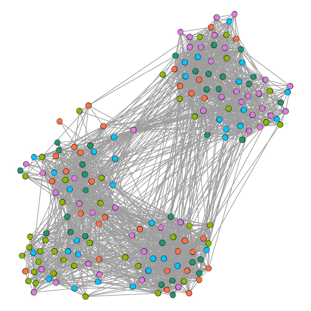
(a) Ground Truth	(b) Result of node2vec	(c) Result of Sub2Vec

Figure 3. Visualization of community detection in dense HighSchool network. Communities obtained by clustering ego-nets vectors returned by Sub2Vec matches the ground truth, while the result from Node2Vec appears to be random.

4.2. Link Prediction

Setup. In this section, we focus on the Link Prediction problem. Given a network $G(V,E)$, the link prediction problem asks to predict the likelihood of formation of an edge between two nodes $v_{1}\in V$ and $v_{2}\in V$, such that $(v_{1},v_{2})\notin E$. It is well known that nodes with common neighbors tend to form future links (Liben-Nowell and Kleinberg, 2007). For example, in a social network two individuals who have multiple friends in common have higher chances of eventually forming a friendship. It is evident from the example that likelihood of future edges depends on the similarity of neighborhood around each end-point. Hence we propose exploiting the embeddings of ego-nets of each node obtained from Sub2Vec to predict whether two nodes will form an edge.

Specifically, we first hide a $P$ percentage of edges randomly sampled from the network, while ensuring that the remaining network remains connected. We consider these “hidden” edges as the ground truth. Then we extract the ego-network, $C_{v}$, for each node $v\in V$. We then run Sub2Vec on $\mathcal{S}=\{C_{v}|v\in V\}$ and use the resulting embedding to predict link. Following methodology in literature (Wang et al., 2016), to evaluate our method, we calculate the Mean Average Precision (MAP). To calculate MAP first we compute Precision@K, as $\text{Precision@k}(v)=\frac{\sum_{i<k}\mathds{1}(v,v_{i})}{k}$. Here $v_{i}$ is the $i^{th}$ node predicted to have edge with node $v$ and $\mathds{1}(v,v_{i})=1$ if $(v,v_{1})$ is in the ground truth, $0$ otherwise. Then we compute the Average Precision as $\text{AP}(v)=\frac{\sum_{i}\text{Precision@i}(v)\cdot\mathds{1}(v,v_{i})}{\sum_{i}\mathds{1}(v,v_{i})}$. Finally, MAP is given as:

$$\text{MAP}=\frac{\sum_{v\in Q}\text{AP}(v)}{|Q|}$$

We compare our result with Node2Vec only as it was previously shown to be better than other baselines (Grover and Leskovec, 2016).

Results. See Table 3. Firstly, note that Sub2Vec outperforms Node2Vec as $P$ varies from 10 to 30 in all the datasets. We also notice that Sub2Vec DM performs surprisingly worse than Node2Vec and Sub2Vec DBON on Facebook. The reason for its poor performance in Facebook is that the network is dense with average clustering co-efficient of 0.6 and effective radius of 4 for 90% of the nodes. Recall that the Sub2Vec DM optimization relies on finding the embedding of the nodes as well, which will not be discriminative for dense networks. In contrast, Sub2Vec DBON learns the features of subgraps directly, without relying on node embeddings, and hence it performs very well on large dense networks including Facebook. Finally we see that Node2Vec consistently improves as $P$ increases, while both versions of Sub2Vec either deteriorate or stagnate. We discuss this more in Section 6.

Table 3. Mean Average Precision for the link prediction task. P is the percentage of edge removed from the network and S stands for Sub2Vec. Winners have been bolded for each dataset. Either Sub2Vec DM or Sub2Vec DBON outperform Node2Vec across all the datasets.

	WorkPlace			HighSchool			Facebook			Astro-PH
$P$	Node2Vec	S DBON	S DM	Node2Vec	S DBON	S DM	Node2Vec	S DBON	S DM	Node2Vec	S DBON	S DM
10	0.25	0.37	0.33	0.39	0.42	0.52	0.50	0.77	0.29	0.12	0.24	0.31
20	0.36	0.28	0.42	0.41	0.52	0.26	0.68	0.84	0.34	0.21	0.31	0.28
30	0.39	0.28	0.40	0.50	0.45	0.57	0.72	0.83	0.35	0.26	0.37	0.44

4.3. Parameter Sensitivity

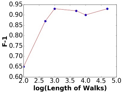
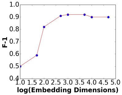
(a) Walk length	(b) Dimension of Vectors

Figure 4. F-1 score on PolBlogs for various values of walk length and dimension of embeddings.

Here we discuss the parameter sensitivity of Sub2Vec. We show how the F-1 score for community detection task on PolBlogs dataset changes when we change the two parameters of Sub2Vec: (i) length of the random walk and (ii) dimension of the embedding. As shown in Figure 4 (a), the F-1 score is 0.85 even when we do random walks of length 500. For the higher length, the F-1 score remains constant.

Similarly, to see how the results of the community detection task changes with the size of the embedding, we run the community detection task on PolBlogs with varying embedding dimension. See Figure 4 (b). The F-1 score saturates when the dimension of vector is greater than 100.

4.4. Scalability

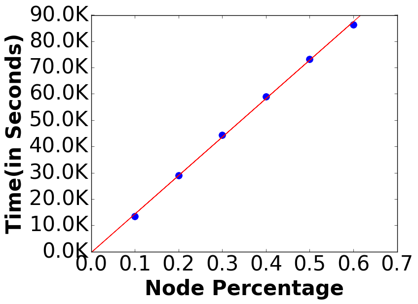
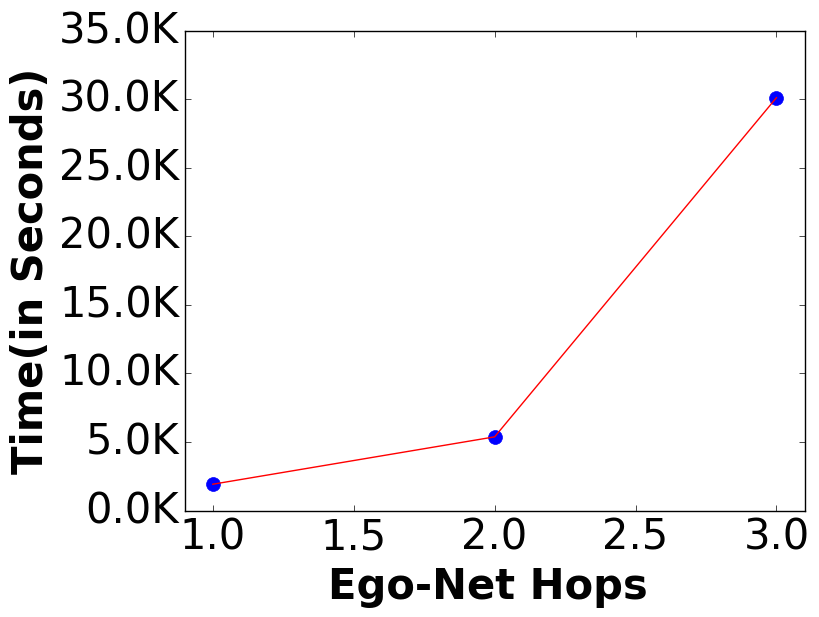
(a) No of Subgraphs	(b) Size of Subgraphs

Figure 5. Scalability w.r.t. number of subgraphs on Youtube and w.r.t size of subgraphs on Astro-PH datasets.

Here we show the scalability of Sub2Vec with respect to the number and the size of subgraphs. We extract connected subgraphs of Youtube dataset of induced by varying percentage of nodes. We then run Sub2Vec on the set of ego-nets in each resulting network. As shown in Figure 5 (a), Sub2Vec is linear w.r.t number of subgraphs. In Figure 5 (b), we run Sub2Vec on 1 to 3 hops ego-nets of Astro-PH dataset. We see a significant jump in the running time when the hop increases from 2 to 3. This is due to the fact that as the hop of ego-net increases, the size of the subgraph increases exponentially due to the low diameter of real world networks.

4.5. Case Studies

We perform case-studies on MemeTracker and DBLP to investigate if our embeddings are interpretable. MemeTracker consists of a series of cascades caused by memes spreading on the network of linked web pages. Each meme-cascade induces a subgraph in the underlying network. We first embed these subgraphs in a continuous vector space by leveraging Sub2Vec. We then cluster these vectors to explore what kind of meme cascade-graphs are grouped together, what characteristics of memes determine their similarity and distance to each other and so on. For this case-study, we pick the top 1000 memes by volume in the data. And we cluster them into 10 clusters using K-Means.

We find coherent clusters which are meaningful groupings of memes based on topics. For example we find cluster of memes related to different topics such as entertainment, politics, religion, technology and so on. Visualization of these clusters is presented in Figure 6. In the entertainment cluster, we find memes which are names of popular songs and movies such as “sweet home alabama”,“somewhere over the rainbow”, “Madagascar 2” and so on. Similarly, we also find a cluster of religious memes. These memes are quotes from the Bible. We also find memes related to politics and religion in the same cluster such as “separation of church and state”’. In politics cluster, we find popular quotes from the 2008 presidential election season e.g. Barack Obama’s popular slogan “yes we can” along with his controversial quotes like “you can put lipstick on a pig” in the cluster. We also find Sarah Palin’s quote like “the chant is drill baby drill”. Similarly, we also find a cluster of technology/video games related memes.

Interestingly, we find that all the memes in Spanish language were clustered together. This indicates that memes in different language travel though separate websites, which matches with the reality as most webpages use one primary language. We also noticed that some of the clusters did not belong to any particular topic. Upon closer examination we found out that these clusters contained memes which were covered by general news website such as msnbc.com, yahoo.com, news.google.com and local news websites such as philly.com from Philadelphia and breakingnews.ie from Ireland.

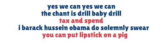
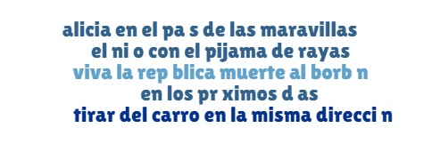
(a) Politics Cluster	(b) Religion Cluster	(c) Spanish Cluster

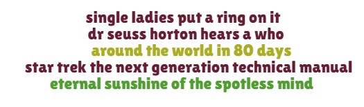
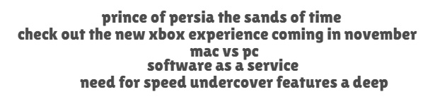
(d) Entertainment Cluster	(e) Technology Cluster

Figure 6. Different Clusters of Memes for the MemeTracker dataset.

For DBLP, we follow the methodology in (Lappas et al., 2010), and extract subgraphs of the coauthorship network based on the keywords contained in the title of the papers.

We include keywords such as ‘classification’, ‘clustering’, ‘xml’, and so on. Once we extract the subgraphs, we run Sub2Vec to learn embedding of these subgraphs. We then project the embeddings down to 2-dimensions using t-SNE (Maaten and Hinton, 2008).

See Figure 7. We see some meaningful groupings in the plot. We see that the keyword related to each other such as ‘graphs’, ‘pagerank’, ‘crawling’, and ‘clustering’ appear together. The classification related keywords such as ‘boosting’, ‘svm’, and ‘classification’ are grouped together. We also see that ‘streams’ and ‘wavelets’ are close to each other. These meaningful groups of keywords highlight the fact that Sub2Vec results in meaningful embeddings.

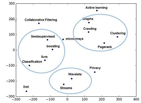
Figure 7. 2D projection of feature vectors learnt by Sub2Vec of subgraphs of DBLP induced by different keywords.

5. Related Work

Network Embedding. The network embedding problem has been well studied. Most of work seeks to generate low dimensional feature representation of nodes. Early work includes Laplacian Eigenmap (Belkin and Niyogi, 2001), IsoMap (Tenenbaum et al., 2000), locally linear embedding (Roweis and Saul, 2000), and spectral techniques (Bach and Jordan, 2003; Chung, 1997). Recently, several deep learning based network embeddings algorithms were proposed to learn feature representations of nodes (Perozzi et al., 2014; Wang et al., 2016; Tang et al., 2015; Grover and Leskovec, 2016). Perozzi et. al (Perozzi et al., 2014) proposed DeepWalk, which extends skip-Gram model (Mikolov et al., 2013) to networks and learns feature representation based on contexts generated by random walks. Grover et. al. proposed a more general method, Node2Vec (Grover and Leskovec, 2016), which generalizes random walks to generate various contexts. SDNE (Wang et al., 2016) and LINE (Tang et al., 2015) learn feature representation of nodes while preserving first and second order proximity. However, all of them learn low dimensional feature vector of nodes, while our goal is to embed subgraphs.

The most similar network embedding literature includes (Riesen and Bunke, 2010; Yanardag and Vishwanathan, 2015; Narayanan et al., 2016). Risen and Bunke propose to learn vector representations of graphs based on edit distance to a set of pre-defined prototype graphs (Riesen and Bunke, 2010). Yanardag et. al. (Yanardag and Vishwanathan, 2015) and Narayanan et al. (Narayanan et al., 2016) learn vector representation of the subgraphs using the Word2Vec (Mikolov et al., 2013) by generating ”corpus” of subgraphs where each subgraph is treated as a word. The above work focuses on some specific subgraphs like graphlets and rooted subgraphs. None of them embed subgraphs with arbitrary structure. In addition, we interpret subgraphs as paragraphs, and leverage the PV-DBOW and PV-DM model (Le and Mikolov, 2014).

Other Subgraph Problems. There has been a lot of work on subgraph related problems. For example, the subgraph discovery problems have been studies extensively. Finding the largest clique is a well-known NP-complete problem (Karp, 1972), which is also hard to approximate (Hstad, 1996). Lee et al. surveyed dense subgraph discovery algorithms for several subgraphs including clique, K-core, K-club, etc (Lee et al., 2010). Akoglu et al. extended the subgraph discovery problem to attributed graphs (Akoglu et al., 2012). Perozzi et al. studied the attributed graph anomaly detection by exploring the neighborhood subgraph of a nodes (Perozzi and Akoglu, 2016). Different from the above works, we seek to find feature representations of subgraphs.

6. Discussion

Table 4. Mean Average Precision for the link prediction task. $P$ is the percentage of edge removed and S stands for Sub2Vec.

	WorkPlace			HighSchool			Facebook			Astro-PH
$P$	Node2Vec	S DBON	S DM	Node2Vec	S DBON	S DM	Node2Vec	S DBON	S DM	Node2Vec	S DBON	S DM
40	0.45	0.32	0.35	0.60	0.47	0.56	0.75	0.78	0.22	0.30	0.39	0.33
50	0.48	0.31	0.33	0.57	0.42	0.49	0.78	0.75	0.12	0.33	0.26	0.34
60	0.50	0.33	0.32	0.60	0.40	0.43	0.79	0.53	0.1	0.34	0.29	0.29

We have shown that Sub2Vec gives meaningful interpretable embeddings of arbitrary subgraphs. We have also shown via our experiments that Sub2Vec outperforms traditional algorithms as well as node-level embedding algorithms for extracting communities from networks, especially in challenging dense graphs. Similarly for link prediction, we also showed that embedding neighborhoods is better for finding correct links.

So for which tasks will Sub2Vec not be ideal? For link prediction, as previously mentioned in Section 4, the performance of Sub2Vec deteriorates when higher percentages of edges are removed from the network. The results for higher percentages, $P$ = 40 to 60, is presented in Table 4. The result shows that Node2Vec outperforms Sub2Vec in such cases, despite performing poorly for lower values of $P$. This happens because, as $P$ increases, the density of the network decreases and results in lesser overlaps in the neighborhoods of nearby nodes. Hence Sub2Vec which preserves the local proximity of subgraphs, does not embed such subgraphs very close to each other, resulting in poorer prediction performance.

We believe, in such situations, perhaps using other proximity measures between subgraphs is more meaningful to preserve during the embedding process than only local proximity.

One such way can be using ‘positional promixity’, where two subgraphs are proximal based on their position in the network. For example, in Figure 2, subgraphs induced by nodes $\{c,d,e\}$ and $\{g,h,j\}$ are similar to each other as the member nodes in these two subgraphs have similar roles. Nodes $e$ and $h$ both connect to central node $f$ and nodes $d$ and $g$ both have degree two. Using just local proximity, these subgraphs are not similar.

Positional Proximity: If we are given two subgraphs $g_{i}(v_{i},e_{1})$ and $g_{j}(v_{j},e_{j})$, then the positional proximity between $g_{i}$ and $g_{j}$ is determined by similarity of position of nodes in $g_{i}$ and $g_{j}$.

Similarly, another way can be using similarity based on structure of subgraphs. For example, in Figure 2, subgraphs induced by nodes $\{a,b,c,e\}$ and $\{h,i,j,k\}$ are similar to each other as both of them are cliques of size four.

Structural Proximity: If we are given two subgraphs $g_{i}(v_{i},e_{1})$ and $g_{j}(v_{j},e_{j})$, then the structural proximity between $g_{i}$ and $g_{j}$ is determined by the structural properties of $g_{i}$ and $g_{j}$.

For link prediction in very sparse networks, Positional Proximity might give more useful embeddings than Local Proximity. We leave the task of embedding subgraphs based on Structural and Positional proximities (or using a combination with Local proximity) and leveraging them for graph mining as future work.

7. Conclusion

We have presented Sub2Vec, a scalable feature learning framework for a set of subgraphs such that the local proximity between them are preserved. In contrast most prior work focused on finding node-level embeddings. We give a theoretical justification and showed that the embeddings generated by Sub2Vec can be leveraged in downstream applications such as community detection and link prediction. We also performed case-studies on two real networks to validate the usefulness of the subgraph features generated by Sub2Vec.

References

- (1)
- Adamic and Glance (2005) Lada A Adamic and Natalie Glance. 2005. The political blogosphere and the 2004 US election: divided they blog. In Proceedings of the 3rd international workshop on Link discovery. ACM, 36–43.
- Akoglu et al. (2012) Leman Akoglu, Hanghang Tong, Brendan Meeder, and Christos Faloutsos. 2012. PICS: Parameter-free identification of cohesive subgroups in large attributed graphs. In Proceedings of the 2012 SIAM international conference on data mining. SIAM, 439–450.
- Bach and Jordan (2003) Francis R Bach and Michael I Jordan. 2003. Learning spectral clustering. In NIPS, Vol. 16.
- Belkin and Niyogi (2001) Mikhail Belkin and Partha Niyogi. 2001. Laplacian eigenmaps and spectral techniques for embedding and clustering. In NIPS, Vol. 14. 585–591.
- Bhagat et al. (2011) Smriti Bhagat, Graham Cormode, and S Muthukrishnan. 2011. Node classification in social networks. In Social network data analytics. Springer, 115–148.
- Blondel et al. (2008) Vincent D Blondel, Jean-Loup Guillaume, Renaud Lambiotte, and Etienne Lefebvre. 2008. Fast unfolding of communities in large networks. Journal of statistical mechanics: theory and experiment 2008, 10 (2008), P10008.
- Chung (1997) Fan RK Chung. 1997. Spectral graph theory. Vol. 92. American Mathematical Soc.
- Fournet and Barrat (2014) Julie Fournet and Alain Barrat. 2014. Contact Patterns among High School Students. PLoS ONE 9, 9 (09 2014), e107878.
- Genois et al. (2015) Mathieu Genois, Christian Vestergaard, Julie Fournet, Andre Panisson, Isabelle Bonmarin, and Alain Barrat. 2015. Data on face-to-face contacts in an office building suggest a low-cost vaccination strategy based on community linkers. Network Science 3 (9 2015), 326–347. Issue 03.
- Girvan and Newman (2002) Michelle Girvan and Mark EJ Newman. 2002. Community structure in social and biological networks. Proceedings of the national academy of sciences 99, 12 (2002), 7821–7826.
- Grover and Leskovec (2016) Aditya Grover and Jure Leskovec. 2016. node2vec: Scalable feature learning for networks. In Proceedings of the 22nd ACM SIGKDD International Conference on Knowledge Discovery and Data Mining. ACM, 855–864.
- Hstad (1996) Johan Hstad. 1996. Clique is hard to approximate within n1. In Proc. 37th Symp. on Found. Comput. Sci. 627–636.
- Karp (1972) Richard M Karp. 1972. Reducibility among combinatorial problems. In Complexity of computer computations. Springer, 85–103.
- Lappas et al. (2010) Theodoros Lappas, Evimaria Terzi, Dimitrios Gunopulos, and Heikki Mannila. 2010. Finding effectors in social networks. In Proceedings of the 16th ACM SIGKDD international conference on Knowledge discovery and data mining. ACM, 1059–1068.
- Le and Mikolov (2014) Quoc V Le and Tomas Mikolov. 2014. Distributed Representations of Sentences and Documents.. In ICML, Vol. 14. 1188–1196.
- Lee et al. (2010) Victor E Lee, Ning Ruan, Ruoming Jin, and Charu Aggarwal. 2010. A survey of algorithms for dense subgraph discovery. In Managing and Mining Graph Data. Springer, 303–336.
- Leskovec et al. (2007) Jure Leskovec, Jon Kleinberg, and Christos Faloutsos. 2007. Graph evolution: Densification and shrinking diameters. ACM Transactions on Knowledge Discovery from Data (TKDD) 1, 1 (2007), 2.
- Leskovec and Mcauley (2012) Jure Leskovec and Julian J Mcauley. 2012. Learning to discover social circles in ego networks. In Advances in neural information processing systems. 539–547.
- Levy and Goldberg (2014) Omer Levy and Yoav Goldberg. 2014. Neural word embedding as implicit matrix factorization. In Advances in neural information processing systems. 2177–2185.
- Liben-Nowell and Kleinberg (2007) David Liben-Nowell and Jon Kleinberg. 2007. The link-prediction problem for social networks. journal of the Association for Information Science and Technology 58, 7 (2007), 1019–1031.
- Maaten and Hinton (2008) Laurens van der Maaten and Geoffrey Hinton. 2008. Visualizing data using t-SNE. Journal of Machine Learning Research 9, Nov (2008), 2579–2605.
- Mikolov et al. (2013) Tomas Mikolov, Ilya Sutskever, Kai Chen, Greg S Corrado, and Jeff Dean. 2013. Distributed representations of words and phrases and their compositionality. In NIPS. 3111–3119.
- Narayanan et al. (2016) Annamalai Narayanan, Mahinthan Chandramohan, Lihui Chen, Yang Liu, and Santhoshkumar Saminathan. 2016. subgraph2vec: Learning distributed representations of rooted sub-graphs from large graphs. arXiv preprint arXiv:1606.08928 (2016).
- Perozzi and Akoglu (2016) Bryan Perozzi and Leman Akoglu. 2016. Scalable anomaly ranking of attributed neighborhoods. In Proceedings of the 2016 SIAM International Conference on Data Mining. SIAM, 207–215.
- Perozzi et al. (2014) Bryan Perozzi, Rami Al-Rfou, and Steven Skiena. 2014. Deepwalk: Online learning of social representations. In Proceedings of the 20th ACM SIGKDD international conference on Knowledge discovery and data mining. ACM, 701–710.
- Riesen and Bunke (2010) Kaspar Riesen and Horst Bunke. 2010. Graph classification and clustering based on vector space embedding. World Scientific Publishing Co., Inc.
- Roweis and Saul (2000) Sam T Roweis and Lawrence K Saul. 2000. Nonlinear dimensionality reduction by locally linear embedding. science 290, 5500 (2000), 2323–2326.
- Sen et al. (2008) Prithviraj Sen, Galileo Mark Namata, Mustafa Bilgic, Lise Getoor, Brian Gallagher, and Tina Eliassi-Rad. 2008. Collective Classification in Network Data. AI Magazine 29, 3 (2008), 93–106.
- Tang et al. (2015) Jian Tang, Meng Qu, Mingzhe Wang, Ming Zhang, Jun Yan, and Qiaozhu Mei. 2015. Line: Large-scale information network embedding. In Proceedings of the 24th International Conference on World Wide Web. ACM, 1067–1077.
- Tenenbaum et al. (2000) Joshua B Tenenbaum, Vin De Silva, and John C Langford. 2000. A global geometric framework for nonlinear dimensionality reduction. science 290, 5500 (2000), 2319–2323.
- Wang et al. (2016) Daixin Wang, Peng Cui, and Wenwu Zhu. 2016. Structural deep network embedding. In Proceedings of the 22nd ACM SIGKDD International Conference on Knowledge Discovery and Data Mining. ACM, 1225–1234.
- Yanardag and Vishwanathan (2015) Pinar Yanardag and SVN Vishwanathan. 2015. Deep graph kernels. In Proceedings of the 21th ACM SIGKDD International Conference on Knowledge Discovery and Data Mining. ACM, 1365–1374.
- Yang and Leskovec (2015) Jaewon Yang and Jure Leskovec. 2015. Defining and evaluating network communities based on ground-truth. Knowledge and Information Systems 42, 1 (2015), 181–213.